Carbon and oxygen in metal-poor halo stars

Carbon and oxygen are key tracers of the Galactic chemical evolution; in particular, a reported upturn in $\mathrm{\left[C/O\right]}$ towards decreasing $\mathrm{\left[O/H\right]}$ in metal-poor halo stars could be a signature of nucleosynthesis by massive Population III stars. We reanalyse carbon, oxygen, and iron abundances in 39 metal-poor turn-off stars. For the first time, we take into account 3D hydrodynamic effects together with departures from local thermodynamic equilibrium (LTE) when determining both the stellar parameters and the elemental abundances, by deriving effective temperatures from 3D non-LTE $\mathrm{H\upbeta}$ profiles, surface gravities from Gaia parallaxes, iron abundances from 3D LTE Fe II equivalent widths, and carbon and oxygen abundances from 3D non-LTE C I and O I equivalent widths. We find that $\mathrm{\left[C/Fe\right]}$ stays flat with $\mathrm{\left[Fe/H\right]}$, whereas $\mathrm{\left[O/Fe\right]}$ increases linearly up to $0.75\,\mathrm{dex}$ with decreasing $\mathrm{\left[Fe/H\right]}$ down to $-3.0\,\mathrm{dex}$. Therefore $\mathrm{\left[C/O\right]}$ monotonically decreases towards decreasing $\mathrm{\left[O/H\right]}$, in contrast to previous findings, mainly because the non-LTE effects for O I at low $\mathrm{\left[Fe/H\right]}$ are weaker with our improved calculations.

1 Introduction

Owing to their different formation sites with different production timescales, the abundance ratios of carbon, oxygen, and iron are key tracers of the chemical evolution of our Galaxy (Tinsley, 1979). Carbon in the cosmos comes from low- and intermediate-mass stars, and through core- and shell-burning in massive stars, and it may be released through core-collapse supernovae as well as through metallicity-dependent stellar winds; oxygen is mainly produced in hydrostatic burning in massive stars and is released through core-collapse supernova; and iron is produced in both core-collapse and type Ia supernova (e.g. Chiappini et al., 2003; Cescutti et al., 2009; Kobayashi & Nomoto, 2009; Karakas & Lattanzio, 2014).

In metal-poor halo stars with $\mathrm{\left[Fe/H\right]}\lesssim-1.5$, the $\mathrm{\left[C/O\right]}$ against $\mathrm{\left[O/H\right]}$ trend has been studied in detail by Akerman et al. (2004) and Fabbian et al. (2009). They found that $\mathrm{\left[C/O\right]}$ decreases with decreasing $\mathrm{\left[O/H\right]}$, down to around $\mathrm{\left[O/H\right]}\approx-1.0$. This is qualitatively consistent with what was found more recently by Nissen et al. (2014) in the less metal-poor halo as well as in thick-disk stars with $\mathrm{\left[Fe/H\right]}\gtrsim-1.5$; there, $\mathrm{\left[C/O\right]}$ decreases from $0.0\,\mathrm{dex}$ at $\mathrm{\left[O/H\right]}\approx 0.2$, down to $-0.45\,\mathrm{dex}$ at $\mathrm{\left[O/H\right]}\approx-0.4$. This trend could signal the presence of a metallicity-dependent carbon yield from the winds of massive stars or an increasing contribution of carbon from low- and intermediate-mass stars with cosmic time.

At lower $\mathrm{\left[O/H\right]}$, Akerman et al. (2004) and Fabbian et al. (2009) found evidence for an overturn in the trend: $\mathrm{\left[C/O\right]}$ increases with further decreasing $\mathrm{\left[O/H\right]}$, reaching $\mathrm{\left[C/O\right]}\approx 0.0$ at $\mathrm{\left[O/H\right]}\approx-3.0$. As discussed in these studies, one interpretation of the change in behaviour in $\mathrm{\left[C/O\right]}$ at low $\mathrm{\left[O/H\right]}$ is that it is a signature of nucleosynthesis by massive Population III stars because the yields of these massive, metal-free first stars are relatively rich in carbon (e.g. Ishigaki et al., 2014). Alternative interpretations are also possible, for example, that it could signal fast stellar rotation in metal-poor Population II stars (Meynet et al., 2006; Chiappini et al., 2006).

However, there are a number of ways that the stellar parameter and elemental abundance determinations of these earlier works can be improved. The effective temperatures, and carbon, oxygen, and iron abundances in these older analyses were based on 1D hydrostatic model atmospheres. Furthermore, while departures from local thermodynamic equilibrium (LTE) were later taken into account for C I and O I, these calculations were based on older atomic data antecedent to modern descriptions of the inelastic collisions with neutral hydrogen (e.g. Barklem, 2016).

Here we revisit the $\mathrm{\left[C/O\right]}$ against $\mathrm{\left[O/H\right]}$ trend in the metal-poor halo. We present for the first time an abundance analysis that is based on both 3D non-LTE stellar parameters and 3D non-LTE elemental abundances that are based on the best atomic data currently available.

2 Method

2.1 Overview

The sample consists of 39 of the 40 stars that have been observed with the VLT/UVES echelle spectrograph by Nissen et al. (2007); G 066-030 was not included here because the stellar parameters we derived ($T_{\mathrm{eff}}=6596\,\mathrm{K}$, $\log{g}=4.70$, $\mathrm{\left[Fe/H\right]}=-1.24$) suggest that the star is a blue straggler (as also suggested by Reggiani et al., 2017). The sample of Fabbian et al. (2009) contains additional stars that are not considered here: G 041-041, G 084-029, and LP 831-070 (for the last of which only an upper limit on the oxygen abundance could be obtained). We only consider the stars from Nissen et al. (2007) in order to base the analysis on a homogeneous set of $\mathrm{H\upbeta}$ observations.

The stellar parameters (effective temperatures, surface gravities, and iron abundances) were determined prior to performing the abundance analysis of carbon and oxygen. They were determined by the separate methods described below, and iterated until consistency was achieved. Following Amarsi et al. (2015), line formation calculations were performed on the stagger-grid of 3D hydrodynamic model atmospheres (Magic et al., 2013), and for comparison also on the standard grid of marcs 1D hydrostatic model atmospheres (Gustafsson et al., 2008). These adopt the solar chemical compositions from Asplund et al. (2009) and Grevesse et al. (2007), respectively, scaled by $\mathrm{\left[Fe/H\right]}$ such that $\mathrm{\left[\upalpha/Fe\right]}=0.4$ for $\upalpha$-elements and $\mathrm{\left[X/Fe\right]}=0.0$ for other elements. These compositions were also assumed in the line formation calculations (except for carbon and oxygen, in Sect. 2.5). This is a reasonable assumption, given that hydrogen is the dominant electron donor across the atmospheres of turn-off stars with $\mathrm{\left[Fe/H\right]}\lesssim-1.5$; We caution, however, that peculiar $\mathrm{\left[Mg/Fe\right]}$ and $\mathrm{\left[Si/Fe\right]}$ abundances may add to the scatter in the more metal-rich part of our sample.

All line formation calculations were performed using the 3D non-LTE radiative transfer code balder (Amarsi et al., 2018b), our custom version of multi3d (Leenaarts & Carlsson, 2009). When using the same stellar parameters and equivalent widths, our 1D LTE carbon and oxygen abundances agree with those of Fabbian et al. (2009) to $0.015\,\mathrm{dex}$, on average; the differences tend to go in the same direction and leave $\mathrm{\left[C/O\right]}$ even less affected. We will present our grids of synthetic 3D non-LTE equivalent widths in a future paper. We list the stellar parameters and abundances in the online Tables 1–4.

2.2 Effective temperature

The effective temperatures were determined by performing profile fits of $\mathrm{H\upbeta}$, using the spectra of Nissen et al. (2007) and the 3D non-LTE grid of Amarsi et al. (2018b). The continuum placement and effective temperature were fit simultaneously by $\chi^{2}$-minimisation, given the surface gravity and iron abundance. The fitting windows included the region within $2.4\,\mathrm{nm}$ from line centre, excluding the region within $0.2\,\mathrm{nm}$ from line centre because the line core forms in the chromosphere and is only poorly modelled by this 3D non-LTE grid.

The new 3D non-LTE effective temperatures tend to be lower than the 1D LTE effective temperatures of Nissen et al. (2007), as expected from the discussion of $\mathrm{H\upbeta}$ in Amarsi et al. (2018b). In general, the difference is larger for the cooler stars (up to $80\,\mathrm{K}$, at $T_{\mathrm{eff}}\approx 5800\,\mathrm{K}$) than for the hotter stars (around $10\,\mathrm{K}$ at $T_{\mathrm{eff}}\approx 6400\,\mathrm{K}$).

2.3 Surface gravity

Stellar masses, effective temperatures, and absolute bolometric magnitudes were used to determine surface gravities as described in Nissen et al. (2007, Sect. 3.2), with two improvements. First, and most important, absolute visual magnitudes were determined based on Gaia DR2 parallaxes (Gaia Collaboration et al., 2018). Two stars have no Gaia parallax available: HD 84937, for which we adopted the HST parallax (VandenBerg et al., 2014), and CD-35 14849, for which the photometric absolute visual magnitude based on Strömgren photometry was used. Second, a newer calibration of the bolometric correction as a function of $V-K$ (Casagrande et al., 2010) was adopted.

Thanks to the high precision of Gaia parallaxes, the new surface gravities are estimated to have RMS errors of about $\pm 0.05\,\mathrm{dex}$. In comparison, the gravities in Nissen et al. (2007) were estimated to have errors of $\pm 0.15\,\mathrm{dex},$ with the main uncertainty arising from errors in the Hipparcos parallaxes and the estimates of absolute magnitudes from Strömgren photometry.

2.4 Iron abundance

The iron abundances were determined from equivalent widths of Fe II lines measured in VLT/UVES echelle spectra (Nissen et al., 2002, 2004, 2007). On average, 16 different optical Fe II lines were available for a given star (only 3 were available for G 064-012 and G 064-037). As the non-LTE effects on Fe II lines are expected to be small (e.g. Amarsi et al., 2016b), the literature equivalent widths were compared to our grid of 3D LTE Fe II equivalent widths. This grid was constructed based on the line parameters from Meléndez & Barbuy (2009). We adopt for the solar iron abundance $\log{\epsilon_{\mathrm{Fe}}}=7.50$ (Asplund et al., 2009), consistent with the 3D model atmospheres.

The new 3D LTE iron abundances tend to be slightly larger than the old 1D LTE abundances, as expected from previous 3D LTE studies (e.g. Amarsi et al., 2016b). The differences tend to be larger for the cooler stars (up to $+0.14\,\mathrm{dex}$) than for the hotter stars ($+0.01\,\mathrm{dex}$).

2.5 Carbon and oxygen abundances

The carbon and oxygen abundances were determined from equivalent widths of C I and O I lines measured in VLT/UVES echelle spectra given in Nissen et al. (2002), Fabbian et al. (2009), and Akerman et al. (2004), in order of preference. The spectra have $R\approx 60000$ and signal-to-noise ratios of $200$ to $300$, and the equivalent widths have precisions of around $0.2\,\mathrm{pm}$; furthermore, the continuum is well defined, as is shown in Fig. 2 of Akerman et al. (2004). The lines are all of high-excitation potential and in the optical/infra-red (C I $906.1\,\mathrm{nm}$, $906.2\,\mathrm{nm}$, $907.8\,\mathrm{nm}$, $908.9\,\mathrm{nm}$, $909.5\,\mathrm{nm}$, $911.2\,\mathrm{nm}$, $940.6\,\mathrm{nm}$; O I $777.2\,\mathrm{nm}$, $777.4\,\mathrm{nm}$, and $777.5\,\mathrm{nm}$). Their sensitivities to the stellar parameters therefore cancel out in the ratio $\mathrm{\left[C/O\right]}$, at least to first order.

The literature equivalent widths were compared to our grids of 1D LTE, 1D non-LTE, 3D LTE, and 3D non-LTE C I and O I equivalent widths. The model C I and O I atoms and 3D non-LTE procedure were recently presented by Amarsi et al. (in prep.) and Amarsi et al. (2018a); the oscillator strengths of the diagnostic lines are from Hibbert et al. (1991, 1993), via the NIST Atomic Spectra Database (Kramida et al., 2015). We adopt for the solar abundances $\log{\epsilon_{\mathrm{C}}}=8.43$ and $\log{\epsilon_{\mathrm{O}}}=8.69$ (Asplund et al., 2009).

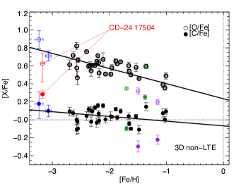
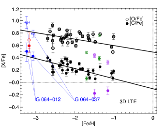
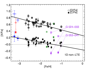
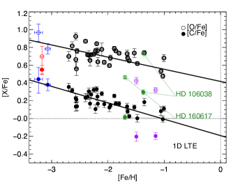
Figure 1: $\mathrm{\left[C/Fe\right]}$ and $\mathrm{\left[O/Fe\right]}$ against $\mathrm{\left[Fe/H\right]}$ for different line formation calculations of ${C\textsc{I}}$ and ${O\textsc{I}}$; $T_{\mathrm{eff}}$, $\log{g}$, and $\mathrm{\left[Fe/H\right]}$ were fixed to their 3D non-LTE values in all four panels. Weighted linear fits are also shown.

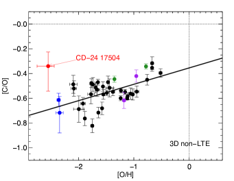
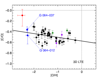
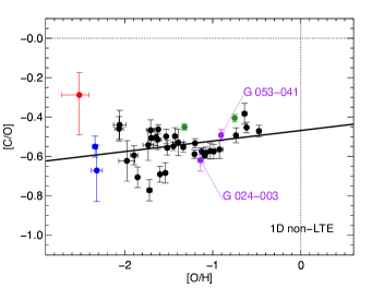
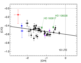
Figure 2: $\mathrm{\left[C/O\right]}$ against $\mathrm{\left[O/H\right]}$ for different line formation calculations of ${C\textsc{I}}$ and ${O\textsc{I}}$; $T_{\mathrm{eff}}$, $\log{g}$, and $\mathrm{\left[Fe/H\right]}$ were fixed to their 3D non-LTE values in all four panels. Weighted linear fits are also shown.

3 Results

We illustrate the results in Fig. 1 and Fig. 2. The error bars indicate the statistical error in the mean based on the line-to-line scatter. The carbon abundance of G 064-012 was determined from a single line, which means that the error bars here reflect an uncertainty of $0.23\,\mathrm{pm}$ on the equivalent width of the C I $909.5\,\mathrm{nm}$ line ($0.87\,\mathrm{pm}$), based on a scatter of $0.32\,\mathrm{pm}$ in the correlation between the measured equivalent widths of the C I $909.5\,\mathrm{nm}$ and $940.6\,\mathrm{nm}$ lines in the rest of the sample. The oxygen abundance of CD-24 17504 was also determined from a single line, therefore the error bars here reflect uncertainties of $+0.11$/$-0.20\,\mathrm{dex}$ in $\mathrm{\left[O/H\right]}$, based on the spectrum analysis of Fabbian et al. (2009, Fig. 4).

Fig. 1 shows that the 3D non-LTE analysis indicates that on average, $\mathrm{\left[C/Fe\right]}$ remains flat with $\mathrm{\left[Fe/H\right]}$, all the way down to $\mathrm{\left[Fe/H\right]}\approx-3.0$, with a mean value of around $0.1\,\mathrm{dex}$. On the other hand, $\mathrm{\left[O/Fe\right]}$ monotonically increases with decreasing $\mathrm{\left[Fe/H\right]}$, with $\mathrm{\left[O/Fe\right]}\approx 0.4$ at $\mathrm{\left[Fe/H\right]}\approx-1.0$, increasing to $\mathrm{\left[O/Fe\right]}\approx 0.75$ at $\mathrm{\left[Fe/H\right]}\approx-3.0$.

Fig. 2 shows that the 1D LTE and 3D LTE $\mathrm{\left[C/O\right]}$ against $\mathrm{\left[O/H\right]}$ trends are very similar: $\mathrm{\left[C/O\right]}$ slightly increases towards lower $\mathrm{\left[O/H\right]}$. In contrast, in non-LTE, $\mathrm{\left[C/O\right]}$ monotonically decreases with decreasing $\mathrm{\left[O/H\right]}$; the gradient is clearly steeper for the 3D non-LTE results than for the 1D non-LTE results.

By comparing the different panels, Fig. 1 also shows that the 3D effects and the non-LTE effects go in the same direction, acting to reduce 3D non-LTE abundances compared to 1D LTE, 3D LTE, and 1D non-LTE; this is consistent with our earlier findings for oxygen (Amarsi et al., 2016a). The 3D non-LTE effects in C I are more severe towards lower $\mathrm{\left[Fe/H\right]}$, whereas the effects in O I are more severe towards higher $\mathrm{\left[Fe/H\right]}$. This drives the steep negative gradient in the 3D non-LTE $\mathrm{\left[C/O\right]}$ trend in Fig. 2 compared to the 1D LTE result.

4 Discussion

Based on the 3D non-LTE results, we find no evidence for an upturn in $\mathrm{\left[C/O\right]}$ at low $\mathrm{\left[O/H\right]}$; rather, $\mathrm{\left[C/O\right]}$ decreases monotonically between $2.6<\mathrm{\left[O/H\right]}<-0.5$. This result is in contrast to the upturn found in the earlier studies of Akerman et al. (2004) and Fabbian et al. (2009). The main reason for the difference with Fabbian et al. (2009) is that our models give far weaker departures from LTE in O I in the metal-poor regime for the reasons discussed in Amarsi et al. (2016a, Sect. 4.2). Thus, in so far as an overturn in the relation would signal Population III nucleosynthesis, we do not find any Population III signature in the $\mathrm{\left[C/O\right]}$ against $\mathrm{\left[O/H\right]}$ plane in this sample of metal-poor halo stars.

It is likely that the mean trends are influenced by an intrinsic cosmic scatter. For instance, HD 106038 and HD 160617 both lie above the mean $\mathrm{\left[C/O\right]}$ trends because of somewhat high $\mathrm{\left[C/Fe\right]}$ and low $\mathrm{\left[O/Fe\right]}$, respectively. The former star may have been influenced by a hypernova event (Smiljanic et al., 2008), while the latter star is boron poor and nitrogen rich (Roederer et al., 2014), whose abundances are probably affected by surface mixing (Pinsonneault, 1997). In addition, although stars G 053-041 and G 024-003 lie near the mean $\mathrm{\left[C/O\right]}$ trends, their $\mathrm{\left[C/Fe\right]}$ and $\mathrm{\left[O/Fe\right]}$ are both lower by roughly $0.2\,\mathrm{dex}$ than the mean trends. The former star was previously found to be sodium enhanced (Nissen & Schuster, 2010) and was likely born in a globular cluster (Ramírez et al., 2012); we speculate that the latter star may have similar origins.

The 1D LTE and 3D non-LTE results both imply that none of the stars in this sample qualify as carbon-enhanced metal-poor stars (CEMP; $\mathrm{\left[C/Fe\right]}>0.7$). The most carbon-enhanced star in the sample is CD-24 17504: our 3D non-LTE result is $\mathrm{\left[C/Fe\right]}=0.28$. This is significantly lower than $\mathrm{\left[C/Fe\right]}=1.1$ reported by Jacobson & Frebel (2015), which was based on a 1D analysis of CH lines in the G band. Similarly, for G 064-012 and G 064-037, we infer $\mathrm{\left[C/Fe\right]}=0.18$ and $\mathrm{\left[C/Fe\right]}=0.10$, respectively, significantly lower than the values of $\mathrm{\left[C/Fe\right]}=1.07$ and $\mathrm{\left[C/Fe\right]}=1.12$ reported by Placco et al. (2016), which were based on a 1D analysis of CH lines in the G band. Molecular features are highly susceptible to 3D effects, with abundance corrections becoming more negative towards lower $\mathrm{\left[Fe/H\right]}$ that are of the right order of magnitude ($0.7$ to $1.1\,\mathrm{dex}$) to bring their results into agreement with ours (e.g. Collet et al., 2006; Gallagher et al., 2017).

Lastly, based on the O I $777\,\mathrm{nm}$ triplet, Fe II lines, and 3D non-LTE stellar parameters, we find that the $\mathrm{\left[O/Fe\right]}$ against $\mathrm{\left[Fe/H\right]}$ trend does not plateau, but shows a clear monotonic decrease with increasing $\mathrm{\left[Fe/H\right]}$. This brings the infra-red triplet into agreement with measurements of UV OH lines in metal-poor red giant stars (Dobrovolskas et al., 2015; Collet et al., 2018). However, it is difficult to reconcile with measurements of the [O I] $630\,\mathrm{nm}$ line in metal-poor stars (Amarsi et al., 2015). We will revisit this oxygen problem in metal-poor stars in a future work.