Symmetry results for the solutions
of a partial differential equation
arising in water waves

Abstract.

This paper recalls some classical motivations in fluid dynamics leading to a partial differential equation which is prescribed on a domain whose boundary possesses two connected components, one endowed with a Dirichlet datum, and the other endowed with a Neumann datum.

The problem can also be reformulated as a nonlocal problem on the component endowed with the Dirichlet datum. A series of recent symmetry results are presented and compared with the existing literature.

1. Introduction

In this paper we present some recent results related to the partial differential equation

$$\begin{cases}\mathrm{div}(y^{a}\nabla v)=0\qquad\text{for}\,\,&x\in\mathbb{R}^{n},y\in(0,1),\\ v_{y}(x,1)=0\qquad&x\in\mathbb{R}^{n},y=1,\\ v(x,0)=u(x)\qquad&x\in\mathbb{R}^{n},y=0,\\ -\displaystyle\lim_{y\rightarrow 0}y^{a}v_{y}=f(v)\qquad&x\in\mathbb{R}^{n},y=0,\end{cases}$$ (1)

with $a\in(-1,1)$. The problem in (1) is related to a water waves model and, in a suitable limit, it recovers a fractional Laplace operator. More precisely, a solution $v$ of (1) can be related to its trace $u$ by a nonlocal equation of the type

$$\mathcal{L}_{a}u=f(u)\qquad\text{in}\,\,\mathbb{R}^{n},$$ (2)

for a suitable linear operator $\mathcal{L}_{a}$. The operator $\mathcal{L}_{a}$ can be written in Fourier modes and will present different asymptotic behaviours for small and large frequencies, making the problem particularly interesting.

One of the main questions that we address is under which conditions the bounded and monotone solutions of (2) are necessarily one-dimensional — that is, as a counterpart, solutions of (1) that are monotone in one of the $x$-variables are necessarily functions only of $x_{1}$ and $y$, up to a rotation.

In Section 2 we recall some basic fluid dynamics motivations to give an elementary but exhaustive description of the problem in (1) in terms of classical physics. Then, in Section 3, we focus on the mathematics relative to (1) and (2), discussing symmetry results in the light of a classical conjecture by Ennio De Giorgi.

2. Physical considerations

In this section, we give a detailed motivation for the problem in (1) arising from a fluid dynamics model. To this end, we consider a possible physical description of an irrotational and inviscid fluid (the “ocean”) in $\mathbb{R}^{n+1}$, though we commonly take $n=2$ in the “real world”. The position of a fluid particle at time $t$ will be denoted by $X(t)=(x(t),y(t))\in\mathbb{R}^{n}\times\mathbb{R}$. We suppose that, at time $t$, the region occupied by the ocean lies above the graph of a function $b(\cdot,t)$ (the “bottom of the ocean”) and below the graph of a function $h(\cdot,t)$ (the “surface of the ocean”). Therefore, in this model, the ocean can be described by the time-dependent domain

$$\Omega(t):=\{(x,y)\in\mathbb{R}^{n}\times\mathbb{R}{\mbox{ s.t. }}b(x,t)\leqslant y\leqslant h(x,t)\},$$ (3)

see Figure 1.

Figure 1. The domain $\Omega(t)$ in (3).

Given a point $X\in\Omega(t)$, we denote by $v(X,t)$ the velocity of the fluid particle at $X$ at time $t$. We denote by $\Phi^{t}(X)$ the evolution produced by the vector field $v$ at time $t$ starting at the point $X$ at time zero, that is the solution of the initial value problem

$$\begin{dcases}&\displaystyle\frac{d}{dt}\Phi^{t}(X)=v(\Phi^{t}(X),t)\qquad{\mbox{ for (small) }}t>0,\\ &\Phi^{0}(X)=X.\end{dcases}$$ (4)

We suppose that the density of the water is described by a positive function $\rho=\rho(X,t)$. Then, the mass of the fluid lying in a region $\widetilde{\Omega}\subset\mathbb{R}^{n+1}$ at time $t$ is described by the quantity

$$\int_{\widetilde{\Omega}}\rho(X,t)\,dX.$$ (5)

The rate at which a fluid mass enters in $\widetilde{\Omega}$ through an infinitesimal portion of $\partial\widetilde{\Omega}$ in the vicinity of a point $X\in\partial\widetilde{\Omega}$ is given by the density times the velocity at $X$ in the direction of the inner normal of $\partial\widetilde{\Omega}$ at $X$. That is, if $\nu(X)$ denotes the exterior normal of $\partial\widetilde{\Omega}$ at $X$, we find that the rate at which a fluid mass enters in $\widetilde{\Omega}$ is given by

$$-\int_{\partial\widetilde{\Omega}}\rho(X,t)\,v(X,t)\cdot\nu(X)\,d{\mathcal{H}}^{n}(X).$$

Comparing with (5), and using the Divergence Theorem, this leads to

$$\int_{\widetilde{\Omega}}\partial_{t}\rho(X,t)\,dX=\frac{d}{dt}\int_{\widetilde{\Omega}}\rho(X,t)\,dX=-\int_{\partial\widetilde{\Omega}}\rho(X,t)\,v(X,t)\cdot\nu(X)\,d{\mathcal{H}}^{n}(X)=-\int_{\widetilde{\Omega}}{\rm div}_{X}\big{(}\rho(X,t)\,v(X,t)\big{)}\,dX.$$

From this, since the volume region $\widetilde{\Omega}$ is arbitrary, we obtain the “mass conservation law” (also known as “continuity equation”) given by

$$\partial_{t}\rho(X,t)+{\rm div}_{X}\big{(}\rho(X,t)\,v(X,t)\big{)}=0\qquad{\mbox{ in }}\;\Omega(t).$$ (6)

Let us now analyze the conditions occurring at the bottom and at the surface of the fluid. At the bottom, we assume that the fluid cannot penetrate inside the ground, hence its velocity is tangent to the seabed. Recalling the notation in (3), we have that $v$ needs to be orthogonal to the normal direction of the graph of $b$, and thus, using the notation $X=(x,y)\in\mathbb{R}^{n}\times\mathbb{R}$,

$$v(X,t)\cdot\big{(}\nabla_{x}b(x,t),-1\big{)}=0\qquad{\mbox{ if }}\;y=b(x,t).$$ (7)

We can therefore collect the results in (6) and (7) by writing

$$\begin{cases}\partial_{t}\rho(X,t)+{\rm div}_{X}\big{(}\rho(X,t)\,v(X,t)\big{)}=0&\qquad{\mbox{ in }}\;\Omega(t),\\ v(X,t)\cdot\big{(}\nabla_{x}b(x,t),-1\big{)}=0&\qquad{\mbox{ on }}\;\{y=b(x,t)\}.\end{cases}$$ (8)

From (8) one sees that the vector field $\rho v$ has perhaps more physical meaning than $v$ alone, since it represents the density speed of the flow, and it is somehow more meaningful to prescribe a bound on $\rho v$ rather than on $v$ itself. For instance, the situation in which $v$ becomes unbounded becomes physically realistic if $\rho v$ remains bounded, since, in this case, roughly speaking, only a very negligible amount of fluid would travel at exceptionally high speed. Therefore, though the equations are perfectly equivalent in case of “nice” vector fields $v$ and densities $\rho$, we prefer to write (8) in a form which makes appear directly the quantity $\rho v$ rather than $v$ alone. This is done by multiplying the identity on the bottom of the ocean by the density, to find

$$\begin{cases}\partial_{t}\rho(X,t)+{\rm div}_{X}\big{(}\rho(X,t)\,v(X,t)\big{)}=0&\qquad{\mbox{ in }}\;\Omega(t),\\ \rho(X,t)\,v(X,t)\cdot\big{(}\nabla_{x}b(x,t),-1\big{)}=0&\qquad{\mbox{ on }}\;\{y=b(x,t)\}.\end{cases}$$ (9)

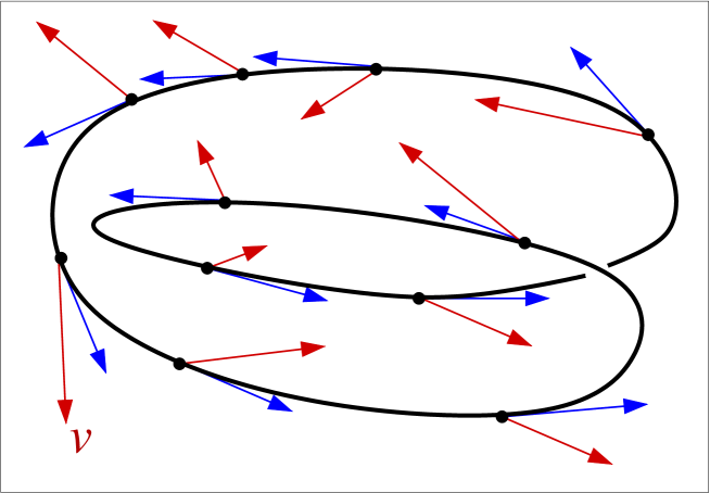
Figure 2. The velocity field $v$ has always a positive component along the tangential direction of the closed curve, hence it is not irrotational.

We also assume that the fluid particles do not “circulate in a cyclone way”, namely that the fluid is irrotational, see Figure 2. To formalize this notion in an arbitrarily large number of dimensions in an elementary geometric way (without using the notion of higher dimensional curls), we assume that, for every fixed time, the integral of the velocity vector field along any closed one-dimensional curve in $\mathbb{R}^{n}$ vanishes. As a matter of fact, it would be enough to require such a condition along polygonal lines, and in fact it would be sufficient to require it along triangular connections.

This irrotationality condition implies (and, in fact, it is equivalent to) that the velocity field admits a potential, namely that there exists a scalar function $u=u(X,t)$ such that

$$v(X,t)=\nabla_{X}u(X,t).$$ (10)

We stress that (10) is a rather striking formula, since it reduces the knowledge of a vector valued function (namely, $v$) to the knowledge of (the derivatives of) a single scalar function. The construction of the potential $u$ is standard, and can be performed along the following argument: we let $\Gamma_{X}$ be the oriented segment starting at the origin and arriving at $X$, and we set

$$u(X,t):=\int_{\Gamma_{X}}v:=\int_{0}^{1}v(\vartheta X,t)\cdot X\,d\vartheta.$$

To prove (10), let $j\in\{1,\dots,n\}$ and $\delta\neq 0$, to be taken arbitrarily small in what follows. We also denote by $\Gamma_{X,\delta,j}$ the oriented segment from $X$ to $X+\delta e_{j}$. Also, given two adjacent segments $\Gamma_{1}$ and $\Gamma_{2}$, we denote by $\Gamma_{1}\cup\Gamma_{2}$ the broken line joining the initial point of $\Gamma_{1}$ to the end point of $\Gamma_{1}$ (which coincides with the initial point of $\Gamma_{2}$) and that to the end point of $\Gamma_{2}$. Furthermore, we denote by $-\Gamma_{1}$ the segment $\Gamma_{1}$ run in the opposite direction. With this notation, we have that $\Gamma_{X+\delta e_{j}}\cup(-\Gamma_{X,\delta,j})\cup(-\Gamma_{X})$ forms a close triangle and accordingly, by the irrotationality condition,

$$0=\int_{\Gamma_{X+\delta e_{j}}\cup(-\Gamma_{X,\delta,j})\cup(-\Gamma_{X})}v=\int_{\Gamma_{X+\delta e_{j}}}v-\int_{\Gamma_{X,\delta,j}}v-\int_{\Gamma_{X}}v$$

$$\qquad=u(X+\delta e_{j},t)-\delta\int_{0}^{1}v(X+\vartheta\delta e_{j},t)\cdot e_{j}\,d\vartheta-u(X,t).$$

Dividing by $\delta$ and sending $\delta\to 0$, we obtain (10), as desired.

Then, inserting (10) into (9), we conclude that

$$\begin{cases}\partial_{t}\rho(X,t)+{\rm div}_{X}\big{(}\rho(X,t)\,\nabla_{X}u(X,t)\big{)}=0&\qquad{\mbox{ in }}\;\Omega(t),\\ \rho(X,t)\,\nabla_{x}u(X,t)\cdot\nabla_{x}b(x,t)-\rho(X,t)\,\partial_{y}u(X,t)=0&\qquad{\mbox{ on }}\;\{y=b(x,t)\}.\end{cases}$$ (11)

We observe that the setting in (1) is a particular case of that in (11), in which one considers the steady case of stationary solutions (i.e. $\rho$ does not depend on time), with $X=(x,y)\in\Omega=\mathbb{R}^{n}\times(0,1)$, and $\rho(X)=y^{a}$, with $a\in(-1,1)$.

Remark 2.1.

Concerning the setting in (4), we recall that in the literature one also considers the “streamlines” of the fluid, described by a parameter $\tau\in\mathbb{R}$, which are (local) solutions of the differential equation (for fixed time $t$)

$$\frac{d}{d\tau}X(\tau,t)=v(X(\tau,t),t).$$

Notice that, if the velocity field $v$ is independent of time, we can actually identify the curve parameter $\tau$ with the usual time $t$ and then the streamlines describe the physical trajectories of the fluid particle. But in general, for velocity fields which depend on time, streamlines do not represent the physical trajectories. Nevertheless, streamlines are always instantaneously tangent to the velocity field of the flow and therefore they indicate the direction in which the fluid particle at a given point travels in time. We maintain the distinction between streamlines and physical trajectories of the flow, and in this note only the latter objects will be taken into account for the main computations.

Remark 2.2.

We point out that in the literature one often assumes that the fluid is “incompressible”, that is, fixed any reference domain $\widetilde{\Omega}$,

$$\frac{d}{dt}\int_{\widetilde{\Omega}}\rho(\Phi^{t}(X),t)\,dX=0.$$

This condition together with (4) leads to

$$\partial_{t}\rho(\Phi^{t}(X),t)+\nabla_{X}\rho(\Phi^{t}(X),t)\cdot v(\Phi^{t}(X),t)=0,$$ (12)

or, equivalently, changing the name of the space variable

$$\partial_{t}\rho(X,t)+\nabla_{X}\rho(X,t)\cdot v(X,t)=0.$$ (13)

The incompressibility condition (13) may be also understood from a “discrete analogue” by thinking that the density $\rho(X,t)$ of a gas formed by indistinguishable molecules at a point $X$ at time $t$ is measured by “counting the number of molecules” in the vicinity of $X$ at time $t$. That is, fixing $r>0$, the gas density could be defined as the number of molecules lying in $B_{r}(X)$ at time $t$. If the gas is incompressible, we expect that the number of molecules around the evolution $\Phi^{t}(X)$ of $X$ remains the same. This gives that

$$\rho(\Phi^{t}(X),t)=\rho(X,0),$$

which leads to (12) and (13).

To appreciate the structural difference between the mass conservation law in (6) and the incompressibility condition in (13), let us consider two examples. In the first example, let

$$v(X,t):=-X\qquad{\mbox{ and }}\qquad\rho(X,t):=e^{nt},$$

with $n>0$. In this case, the velocity field pushes all the fluid towards the origin, preserving the mass according to (6): as a consequence, the particles of the fluid get “packed” and their density increases, and the incompressibility condition (13) is indeed violated.

As a second example, let us consider the case in which

$$v(X,t):=-X\qquad{\mbox{ and }}\qquad\rho(X,t):=1.$$

In this case, the fluid elements are still pushed towards the origin, but the density remains constant. This means that there must be a leak somewhere, from which the fluid escapes. In this situation, the incompressibility condition in (13) is satisfied, but the mass is lost and accordingly (6) does not hold.

We also point out that if the the mass conservation law in (6) and the incompressibility condition in (13) are both satisfied, then

$$0 = \partial_{t}\rho(X,t)+{\rm div}_{X}\big{(}\rho(X,t)\,v(X,t)\big{)}$$

$$= \partial_{t}\rho(X,t)+\nabla_{X}\rho(X,t)\cdot v(X,t)+\rho(X,t)\,{\rm div}_{X}\,v(X,t)$$

$$= \rho(X,t)\,{\rm div}_{X}\,v(X,t),$$

and, as a consequence,

$${\rm div}_{X}\,v(X,t)=0\qquad{\mbox{ in }}\;\Omega(t).$$

In this note, we will not explicitly take into account incompressibility assumptions, but merely the conservation of mass in (6).

Remark 2.3.

Concerning the top surface of the fluid, in the literature it is often assumed that fluid particles on this surface remain there forever (i.e., there is no “mixing effect” between the top surface of the sea and the rest of the water mass). This condition, in the notation of (3) and (4), would translate into

$$\Phi^{t}_{2}(X)=h(\Phi_{1}^{t}(X),t),$$

as long as $X=(x,y)$ and $y=h(x,0)$, where $\Phi^{t}(X)=\big{(}\Phi^{t}_{1}(X),\Phi^{t}_{2}(X)\big{)}\in\mathbb{R}^{n}\times\mathbb{R}$. Hence, in view of (4),

$$0=\frac{d}{dt}\Big{(}h(\Phi_{1}^{t}(X),t)-\Phi^{t}_{2}(X)\Big{)}=v(\Phi^{t}(X),t)\cdot\big{(}\nabla_{x}h(\Phi^{t}_{1}(X),t),\,-1\big{)}+\partial_{t}h(\Phi_{1}^{t}(X),t).$$

In this note, we do not need to assume this additional no mixing condition.

3. Symmetry results

Now, we present some results for an elliptic problem related to the stationary case of the model introduced in Section 2. Besides assuming no dependence on time $t$, we also consider the simplification of a “flat ocean”, by taking $b(x)=H>0$ and $h(x)=0$ (recall the notation in (3)). This choice implies that we now consider the sea as

$$\Omega=\{(x,y)\in\mathbb{R}^{n}\times\mathbb{R}{\mbox{ s.t. }}0\leqslant y\leqslant H\},$$

and that we are “reversing the vertical direction”, in order to have the ocean surface on $\{y=0\}$. This last simplification is done for pure mathematical convenience and does not affect the model.

In our setting, we can use (11) in order to associate a velocity potential in the whole slab $\mathbb{R}^{2}\times[0,H]$ with a given datum on the surface of the ocean. Given the values of the velocity potential on $\{y=0\}$ and denoting such datum by $u$, we consider the velocity potential $v$ in the whole slab $\mathbb{R}^{2}\times[0,H]$ that solves

$$\begin{cases}0={\rm div}(\varrho V)={\rm div}(\varrho\nabla v)\quad&{\mbox{ in }}\mathbb{R}^{2}\times(0,H),\\ 0=V_{3}\big{|}_{y=H}=v_{y}\big{|}_{y=H}\quad&{\mbox{ on }}\mathbb{R}^{2}\times\{y=H\},\\ v=u\big{|}_{y=0}\quad&{\mbox{ on }}\mathbb{R}^{2}\times\{y=0\}.\end{cases}$$ (14)

In relation to water waves and in view of the discussion in Section 2, we are interested in the weighted vertical velocity on the surface of the ocean. Thus, the operator that we want to study is

$$\mathcal{L}_{a}u(x):=-\displaystyle\lim_{y\rightarrow 0}\rho(y)v_{y}(x,y).$$ (15)

When $\varrho:=1$ and $H\to+\infty$ (which is the case of a fluid with constant density and an “infinitely deep sea”), the operator $\mathcal{L}_{a}$ is the square root of the Laplacian, see e.g. [CS]. For finite values of $H$ the operator described in (15) is nonlocal, but also not of purely fractional type, as we are going to see.

In the following, we choose

$$\varrho(y):=y^{a}$$ (16)

as a density, where $a\in(-1,1)$. We notice that, in this case,

the limit as $$H\to+\infty s$$ corresponds to the -th root of the Laplacian, (17)

with $s:=(1-a)/2$, but for a finite value of $H$ the problem is not of purely fractional type. From now on, we normalize the domain by setting $H:=1$. From a physical point of view, the choice in (16) corresponds to the situation in which the density of the fluid at a point depends only on the depth, in a power-like fashion, and it is constant in the horizontal directions. Possibly, some of the results that we present here can be extended to the case of a more general density $\rho(y)$, and we intend to investigate the possibility of this generalization in a forthcoming work.

After generalizing the physical setting $\mathbb{R}^{2}\times[0,1]$ to the mathematically interesting case $\mathbb{R}^{n}\times[0,1]$ — with coordinates $x\in\mathbb{R}^{n}$ and $y\in[0,1]$ — the extension problem in (14) reads

$$\begin{cases}\mathrm{div}(y^{a}\nabla v)=0\qquad&\text{in}\,\,\mathbb{R}^{n}\times(0,1),\\ v_{y}(x,1)=0\qquad&\text{on}\,\,\mathbb{R}^{n}\times\{y=1\},\\ v(x,0)=u(x)\qquad&\text{on}\,\,\mathbb{R}^{n}\times\{y=0\}.\end{cases}$$ (18)

Therefore, in light of (16), the Dirichlet to Neumann operator $\mathcal{L}_{a}$ in (15) is given by

$$\mathcal{L}_{a}u(x)=-\displaystyle\lim_{y\rightarrow 0}y^{a}v_{y}(x,y),$$

and, for a given nonlinearity $f\in C^{1,\gamma}(\mathbb{R})$, we want to study the equation

$$\mathcal{L}_{a}u(x)=f(u)\qquad\text{in}\,\,\mathbb{R}^{n}.$$ (19)

As a technical remark, we notice that, in order to have the operator $\mathcal{L}_{a}$ well defined for every smooth function $u:\mathbb{R}^{n}\to\mathbb{R}$, we need to choose the extension $v$ in (18) in a unique way. Indeed, for example, if $v$ is a solution of (18) with $a=0$, then so is the function $v(x,y)+e^{\pi x/2}\sin(\pi y/2)$. To overcome this problem and uniquely determine $v$ in (18), we choose among all the possible solutions of (18) the one which is a minimizer of the energy

$$\mathscr{E}_{a}(w):=\int_{\mathbb{R}^{n}\times(0,1)}y^{a}\left\lvert\nabla w(x,y)\right\rvert^{2}\,dx\,dy,$$ (20)

in the class of all the functions $w\in W^{1,2}(\mathbb{R}^{n}\times(0,1),y^{a})$ such that $w(x,0)=u(x)$. Such a minimizer $v$ exists, it is unique, due to the convexity of the energy functional in (20), and it solves the problem in (18) — see [MV] for all the details.

With the setting in (18), the problem in (19) can be formulated in the following way:

$$\begin{cases}\mathrm{div}(y^{a}\nabla v)=0\qquad&\text{in}\,\,\mathbb{R}^{n}\times(0,1),\\ v_{y}(x,1)=0\qquad&\text{on}\,\,\mathbb{R}^{n}\times\{y=1\},\\ -\displaystyle\lim_{y\rightarrow 0}y^{a}v_{y}=f(v)\qquad&\text{on}\,\,\mathbb{R}^{n}\times\{y=0\},\end{cases}$$ (21)

where $f\in C^{1,\gamma}(\mathbb{R})$ with $\gamma>0$.

Problem (21) has a variational structure, since solutions of (21) correspond to critical points of the energy functional

$$\mathcal{E}(v):=\frac{1}{2}\int_{\mathbb{R}^{n}\times(0,1)}y^{a}|\nabla v(x,y)|^{2}\,dx\,dy+\int_{\mathbb{R}^{n}\times\{y=0\}}F(v(x,0))\,dx,$$ (22)

where the associated potential $F$ is such that $F^{\prime}=-f$.

Since problem (21) is set in a slab of fixed height, it is technically convenient to localize the energy functional on cylinders. Namely, we define the cylinder

$$C_{R}:=B_{R}\times(0,1),$$ (23)

where $B_{R}\subset\mathbb{R}^{n}$ denotes the ball of radius $R$ centered at $0$. Then, by (22), the localized energy functional associated to problem (21) reads

$$\mathcal{E}_{R}(v):=\frac{1}{2}\int_{C_{R}}y^{a}|\nabla v(x,y)|^{2}\,dx\,dy+\int_{B_{R}\times\{y=0\}}F(v(x,0))\,dx.$$

In particular, the potential $F$ is naturally defined up to an additive constant, hence, focusing on bounded solutions, we can also suppose that $F\geqslant 0$. For this kind of problems, the model case is the nonlinearity $f(t):=t-t^{3}$, which arises in the study of phase transitions and it is the derivative of the double-well potential

$$F(t)=\frac{1}{4}\left(1-t^{2}\right)^{2}.$$

The usual notions of minimizer of the energy and of stable solution to problem (21) can be defined in a standard way. We say that a bounded function $v\in C^{1}(\mathbb{R}^{n}\times(0,1))$ is a minimizer for (21) if

$$\mathcal{E}_{R}(v)\leqslant\mathcal{E}_{R}(w)$$

for every $R>0$ and for every bounded competitor $w$ such that $v\equiv w$ on $\partial B_{R}\times(0,1)$.

We say that a bounded solution $v$ of (21) is stable if the second variation of the energy is non-negative, i.e.

$$\int_{\mathbb{R}^{n}\times[0,1]}y^{a}\lvert\nabla\xi\rvert^{2}\,dx\,dy-\int_{\mathbb{R}^{n}\times\{y=0\}}f^{\prime}(u)\xi^{2}\,dx\geqslant 0$$

for every function $\xi\in C_{0}^{1}(\mathbb{R}^{n}\times[0,1])$.

Clearly, if $v$ is a minimizer for (21) then, in particular, it is a stable solution. Another important subclass of stable solutions that we consider in this paper is given by the monotone solutions of (21). We say that a solution $v$ of (21) is monotone if it is strictly monotone in one horizontal direction, say $\partial_{x_{n}}v>0$. For this kind of problems, it is possible to prove that monotone solutions are stable using a non-variational characterization of stability — see for example Lemma 3.1 in [CMV] for all the details. See also [MR2779463] for a complete introduction to stable solutions in elliptic PDEs.

Problem (21) was initially studied by de la Llave and the third author in [DllV] with constant density, so with $a=0$. In particular, they proved a Liouville theorem that assures the one-dimensional symmetry of monotone solutions on the trace, provided that a suitable energy estimate for the functional associated to the problem holds true. Since this energy estimate in dimension $n=2$ is a direct consequence of a classical gradient bound, they obtain that monotone solutions of (21) with $a=0$ depend on only one horizontal variable if $n=2$.

We now describe some recent symmetry and rigidity results for problem (21) in the light of a long-lasting line of investigation that was opened by a celebrated conjecture by Ennio De Giorgi.

3.1. Symmetry properties for the Allen-Cahn equation

One of the main interests in proving the one-dimensional symmetry of monotone solutions comes from a conjecture formulated by Ennio De Giorgi for the classical Allen-Cahn equation. Indeed, in 1979 De Giorgi posed the following question.

Conjecture 3.1.

Let $u$ be a bounded and smooth solution of the Allen-Cahn equation

$$-\Delta u=u-u^{3}\qquad\text{in}\,\,\mathbb{R}^{n},$$

such that $\partial_{x_{n}}u>0$. Is it true that, if $n\leqslant 8$, then $u$ is one-dimensional?

A heuristic motivation of the conjecture can be formulated in light of the work of Modica and Mortola [MM]. Indeed, they proved that a proper rescaling of the energy functional associated to the Allen-Cahn equation $\Gamma$-converges to the perimeter functional, as the rescaling parameter goes to zero. This means that a proper rescaling of the minimizers of the Allen-Cahn equation converges to characteristic functions of sets of minimal perimeter. The threshold dimension $n=8$ comes from the fact that super-level sets of monotone functions are expected to be epigraphs (though this is a tricky point, see e.g. formula (5) in [FV]), and minimal graphs are flat if $n\leqslant 8$. For a complete discussion of minimal surfaces, see the illuminating monograph [G].

Summing up, the above heuristic argument would give that, at least in dimension $n\leqslant 8$, if we look at monotone solutions “from very far” (through a rescaling), their level sets are close to hyperplanes. The question in Conjecture 3.1 asks if, for this to hold, the level sets of the function must be necessarily parallel hyperplanes.

The conjecture of De Giorgi remained unanswered in every dimension $n$ for almost twenty years. It was proved to hold if $n=2$ by Ghoussoub and Gui [GG] and by Berestycki, Caffarelli and Nirenberg [MR1655510], and if $n=3$ by Ambrosio and Cabré [AC]. Regarding dimensions $4\leqslant n\leqslant 8$, Savin proved in [S] the conjecture by assuming the following additional hypothesis about the limits in the monotone direction

$$\lim_{x_{n}\to\pm\infty}u(x^{\prime},x_{n})=\pm 1.$$ (24)

Condition (24) can be weakened by assuming two-dimensional symmetry of the profiles at infinity, see [MR2728579].

As a counterpart of the results giving positive answers to Conjecture 3.1 (possibly under additional assumptions), del Pino, Kowalczyk and Wei provided in [dPKW] an example of a monotone solution to the Allen-Cahn equation in dimension $n=9$ which is not one-dimensional. In this way, they proved that dimension $n=8$ in Conjecture 3.1 is the optimal one.

We refer to [FV, CW] for more detailed surveys on topics related to Conjecture 3.1.

3.2. Symmetry properties for the fractional Allen-Cahn equation

The fractional analogue of Conjecture 3.1 can be formulated as follows:

Conjecture 3.2.

Let $s\in(0,1)$ and $u$ be a bounded and smooth solution of the fractional Allen-Cahn equation

$$(-\Delta)^{s}u=u-u^{3}\qquad\text{in}\,\,\mathbb{R}^{n},$$ (25)

such that $\partial_{x_{n}}u>0$. Is it true that, if $n$ is sufficiently small, then $u$ is one-dimensional?

This question is also motivated by an analogue in the fractional setting of the $\Gamma$-convergence result by Modica and Mortola. Indeed, the third author and Savin proved in [SV] that a proper rescaling of the energy associated to (25) $\Gamma$-converges to the classical perimeter if $s\in\left[\frac{1}{2},1\right)$ and to the fractional perimeter if $s\in\left(0,\frac{1}{2}\right)$.

The fractional perimeter was introduced by Caffarelli, Roquejoffre and Savin in [CRS], and — without going into the details — can be thought as a nonlocal version of the classical perimeter, counting the interactions between points which lie in the two separated sides of the boundary of the set. As in the classical case, one could relate, at least at a level of motivations, the validity of Conjecture 3.2 to the regularity and rigidity properties of the minimizers of the limit energy functional, namely to the classical minimal surfaces when $s\in\left[\frac{1}{2},1\right)$, and to the nonlocal minimal surfaces when $s\in\left(0,\frac{1}{2}\right)$. With respect to this, we recall that nonlocal minimal surfaces are known to be smooth only in dimension $2$ — see [MR3090533] — and up to dimension $7$ provided that $s\in\left[\frac{1}{2}-\varepsilon_{0},\frac{1}{2}\right)$ and $\varepsilon_{0}$ is sufficiently small — see [MR3107529]. Nonlocal minimal surfaces that are entire graphs are known to be necessarily hyperplanes only in dimension $2$ and $3$, and up to up to dimension $8$ provided that $s\in\left[\frac{1}{2}-\varepsilon_{0},\frac{1}{2}\right)$ and $\varepsilon_{0}$ is sufficiently small — see [MR3680376]. Till now, no singular minimal surface is known — see however [MR3798717] for the construction of a singular cone in dimension $7$ which is a stable critical point of the fractional perimeter when $s$ is sufficiently small.

Of course, this lack of knowledge for the nonlocal minimal surfaces (when compared to the classical minimal surfaces) provides a series of conceptual difficulties when dealing with Conjecture 3.2, especially in the regime $s\in\left(0,\frac{1}{2}\right)$.

The problem posed by Conjecture 3.2 was solved in dimension $n=2$ by Cabré and Solà-Morales in [CSM] for $s=\frac{1}{2}$, and then by Cabré, Sire and the third author in [YV, CY2] for every $s\in(0,1)$.

A positive answer in dimension $n=3$ was given by Cabré and Cinti in [CC1] and [CC2] in the cases $s=\frac{1}{2}$ and $s\in\left(\frac{1}{2},1\right)$, respectively. Regarding the strongly nonlocal regime, namely when $s\in(0,\frac{1}{2})$, recently the conjecture has been proved in dimension $n=3$ by Farina and the first and the third authors in [DFV] (using an improvement of flatness result by [XFAH]) and by Cabré, Cinti and Serra in [CCS] (by a different approach which relies on some sharp energy estimates and a blow-down convergence result for stable solutions).

Very recently, Figalli and Serra proved in [FS] Conjecture 3.2 to be true for $s=\frac{1}{2}$ and $n=4$ (also providing one-dimensional symmetry of stable solutions in dimension $n=3$).

Concerning higher dimensions, Savin proved in [S1, S2] the conjecture for $4\leqslant n\leqslant 8$ and $s\in\left[\frac{1}{2},1\right)$ under the additional assumption (24). Moreover, in [XFAH] it has been proved that Conjecture 3.2 is true in dimensions $4\leqslant n\leqslant 8$ if $s\in\left[\frac{1}{2}-\varepsilon_{0},\frac{1}{2}\right)$, for some $\varepsilon_{0}$ sufficiently small, under the additional assumption (24).

Besides these results, Conjecture 3.2 is also open in its generality, and the critical dimension might depend on the fractional parameter $s$.

3.3. Symmetry properties for the water wave problem

Since, in our framework, we are dealing with a generalization of fractional Laplace operators, which are attained in the limit according to (17), a natural counterpart of Conjecture 3.2 is the following one:

Conjecture 3.3.

Let $a\in(-1,1)$ and $u$ be a bounded and smooth solution of the fractional Allen-Cahn equation

$${\mathcal{L}}_{a}u=u-u^{3}\qquad\text{in}\,\,\mathbb{R}^{n},$$

such that $\partial_{x_{n}}u>0$. Is it true that, if $n$ is sufficiently small, then $u$ is one-dimensional?

Conjecture 3.3 is related to, but structurally different from, Conjecture 3.2. As a matter of fact, to point out the differences between problem (19)-(21) treated in these notes and its analogue for the fractional Laplacian, we consider the Fourier transform of the Dirichlet to Neumann operator $\mathcal{L}_{a}$. It can be computed as

$$\widehat{\mathcal{L}_{a}(u)}(\xi)=c_{1}(s)\frac{J_{1-s}(-i\left\lvert\xi\right\rvert)}{\cos\left(s\pi\right)J_{1-s}(-i\left\lvert\xi\right\rvert)+\sin\left(s\pi\right)Y_{1-s}(-i\left\lvert\xi\right\rvert)}\left\lvert\xi\right\rvert^{2s}\widehat{u}(\xi),$$

where $J_{m}(\cdot)$ and $Y_{m}(\cdot)$ are the Bessel functions of order $m$, respectively of the first and second kind, and $c_{1}(s)$ is a constant depending only on $s\in(0,1)$. As customary, the symbol $\widehat{u}$ denotes the Fourier transform of $u$.

Therefore, the operator $\mathcal{L}_{a}$ can be seen as a Fourier operator with symbol

$$S_{s}(\xi):=c_{1}(s)\frac{J_{1-s}(-i\left\lvert\xi\right\rvert)}{\cos\left(s\pi\right)J_{1-s}(-i\left\lvert\xi\right\rvert)+\sin\left(s\pi\right)Y_{1-s}(-i\left\lvert\xi\right\rvert)}\left\lvert\xi\right\rvert^{2s}.$$

The symbol $S_{s}(\xi)$ was already known in [BV, DllV] in the special case $s=\frac{1}{2}$ as

$$S_{1/2}(\xi)=\frac{e^{\left\lvert\xi\right\rvert}-e^{-\left\lvert\xi\right\rvert}}{e^{\left\lvert\xi\right\rvert}+e^{-\left\lvert\xi\right\rvert}}\left\lvert\xi\right\rvert$$

and it has been computed later by the second and third author in [MV] for every fractional parameter $s\in(0,1)$. By evaluating the limits of $S_{s}(\xi)$ as $\left\lvert\xi\right\rvert$ goes to zero and infinity, we observe that

$$S_{s}(\xi)\sim\left\lvert\xi\right\rvert^{2}\qquad \text{as}\,\,\left\lvert\xi\right\rvert\to 0;$$ (26)

$$S_{s}(\xi)\sim\left\lvert\xi\right\rvert^{2s}\qquad \text{as}\,\,\left\lvert\xi\right\rvert\to+\infty.$$

This fact is already evident in the simpler case $s=\frac{1}{2}$, but it can be shown also in the general case $s\in(0,1)$ — see again [MV] for all the details. To better undestand the implications of this behaviour, we should remind that $\left\lvert\xi\right\rvert^{2}$ is the symbol of the classical Laplacian, and that the fractional Laplacian can be also written in the Fourier setting as

$$\widehat{(-\Delta)^{s}u}(\xi)=\left\lvert\xi\right\rvert^{2s}\widehat{u}(\xi),$$

see for example [H]. Looking at the asymptotics (26), it becomes evident that the operator $\mathcal{L}_{a}$ is not of purely fractional type, and, in fact, it shows a nonlocal behaviour for high frequencies but it becomes similar to the Laplacian for small frequencies.

In this setting, Conjecture 3.3 was first addressed by de la Llave and the third author in [DllV], for the special case $a=0$. As mentioned above, their main result is a Liouville theorem, that gives one-dimensional symmetry of monotone solutions under an assumption about the growth of the Dirichlet energy of the solution. In this way, they establish Conjecture 3.3 for $a=0$ and $n=2$ — see in particular Theorem 1 in [DllV].

The results in [DllV] have been extended in [CMV] from monotone to stable solutions, also considering all the fractional parameters $a\in(-1,1)$ and not only $a=0$. In this setting, the result in [CMV] reads as follows.

Theorem 3.4.

Let $f\in C^{1,\gamma}(\mathbb{R})$, with $\gamma>\max\{0,-a\}$, and let $v$ be a bounded and stable solution of (21).

Suppose that there exists $C>0$ such that

$$\int_{C_{R}}y^{a}|\nabla_{x}v(x,y)|^{2}\,dx\,dy\leqslant CR^{2}$$ (27)

for any $R\geqslant 2$, where the notation in (23) has been used.

Then, there exist $v_{0}:\mathbb{R}\times(0,1)\rightarrow\mathbb{R}$ and $\omega\in{\rm S}^{n-1}$ such that

$$v(x,y)=v_{0}(\omega\cdot x,y)\qquad{\mbox{ for any $(x,y)\in\mathbb{R}^{n}\times(0,1)$.}}$$

In particular, the trace $u$ of $v$ on $\{y=0\}$ can be written as $u(x)=u_{0}(\omega\cdot x)$.

Finally, either $u_{0}^{\prime}>0$ or $u_{0}^{\prime}\equiv 0$.

Remark 3.5.

For this kind of elliptic problems, it is a standard fact that bounded solutions have bounded gradients, see for example [GT]. For this reason, if we assume $n=2$, then hypothesis (27) is trivially verified by any bounded stable solution. Therefore, we deduce that bounded stable solutions of (21) are one-dimensional on the trace if $n=2$. In particular, this implies the validity of Conjecture 3.3 in dimension $n=2$, for all $a\in(-1,1)$ as a corollary of Theorem 3.4.

In [CMV], Conjecture 3.3 is also addressed when $n=3$. For this, the strategy is based on energy estimates and the use of Theorem 3.4. Namely, in [CMV] the following result is proved:

Theorem 3.6 (Energy estimate for minimizers).

Let $f\in C^{1,\gamma}(\mathbb{R})$, with $\gamma>\max\{0,-a\}$, and let $v$ be a bounded minimizer for problem (21).

Then, we have

$$\mathcal{E}_{R}(v)=\frac{1}{2}\int_{C_{R}}y^{a}\lvert\nabla v\rvert^{2}\,dx\,dy+\int_{B_{R}\times\{y=0\}}F(v)\,dx\leqslant CR^{n-1},$$ (28)

for any $R\geqslant 2$, where the notation in (23) has been used.

We point out that (28) holds in general for minimizers of the energy associated to problem (21) in every dimension $n$, but the application to symmetry problems usually becomes relevant only in dimension $n\leqslant 3$. Let us give now a brief look at the proof of Theorem 3.6, which is based on a direct comparison. Indeed, since we are assuming that $v$ is a minimizer, for every admissible competitor $w$ it holds that

$$\mathcal{E}_{R}(v)\leqslant\mathcal{E}_{R}(w).$$

We say that a competitor $w$ is admissible if $w\equiv v$ on the lateral boundary $\partial B_{R}\times(0,1)$. The key point for the proof is defining a competitor $\widetilde{w}$ constantly equal to the minimum of the potential $F$ in a cylinder of radius $R-1$, and then cutting it off in order to make it admissible. In such a way, one is able to estimate the energy of $\widetilde{w}$ in a cylinder of radius $R$ and obtain (28). A strategy of this type has been used also in [AC] to solve the classical De Giorgi conjecture in dimension $n=3$.

Restricting to the case $n=3$, it is possible to prove the same estimate in Theorem 3.6 for bounded solutions whose traces on $\{y=0\}$ are monotone in some direction, according to the following result:

Theorem 3.7 (Energy estimate for monotone solutions for $n=3$).

Let $f\in C^{1,\gamma}(\mathbb{R})$, with $\gamma>\max\{0,-a\}$, and let $v$ be a bounded solution of (21) with $n=3$ such that its trace $u(x)=v(x,0)$ is monotone in some direction.

Then, we have

$$\mathcal{E}_{R}(v)=\frac{1}{2}\int_{C_{R}}y^{a}\lvert\nabla v\rvert^{2}\,dx\,dy+\int_{B_{R}\times\{y=0\}}F(v)\,dx\leqslant CR^{2},$$

for any $R\geqslant 2$, where the notation in (23) has been used.

We stress the fact that this energy estimate holds for monotone solutions of (21) only if we are in the case $n=3$. As mentioned above, this is due to the proof, and in particular to the fact that we know from Remark 3.5 that stable solutions enjoy rigidity properties when we are in one dimension less, i.e. when $n=2$.

Let us briefly sketch the proof of Theorem 3.7. The interested reader can find all the details in Section 5 of [CMV]. First, it is necessary to define the two limit profiles of the monotone solution $v$. Indeed, since $v$ is monotone in one direction, say $v_{x_{3}}>0$, we can define

$$\underline{v}(x_{1}.x_{2},y):=\lim_{x_{3}\to-\infty}v(x,y);$$

$$\overline{v}(x_{1},x_{2},y):=\lim_{x_{3}\to+\infty}v(x,y).$$

These functions are well defined for the monotonicity hypothesis, they are solutions of (21) in one dimension less, so with $n=2$, and in particular they are stable. Here the dimension plays a key role, since we can use Theorem 3.4 and deduce that $\underline{v}$ and $\overline{v}$ are one-dimensional functions on the trace. From the existence of such solutions, it is possible to characterize the potential $F$. This is something that is fundamental in the proof.

On the other side, a monotone solution $v$ is a minimizer of the energy in the class

$$\mathcal{A}_{v}:=\left\{w\in H^{1}(C_{R};y^{a})\,\,\text{such that}\,\,w=v\,\,\text{on}\,\,\partial B_{R}\times(0,1)\,\,\text{and}\,\,\underline{v}\leqslant w\leqslant\overline{v}\,\,\text{in}\,\,C_{R}\right\}.$$

For the detailed proof of this fact in the setting of water waves, see Lemma 5.6 in [CMV].

At this point, one can use the characterization of the potential $F$ provided by the previous steps in order to show that the competitor used in the proof of Theorem 3.6 belongs to the class $\mathcal{A}_{v}$, i.e. $\widetilde{w}\in\mathcal{A}_{v}$. Since the energy of $\widetilde{w}$ in $C_{R}$ can be bounded by $CR^{2}$, this finishes the proof of Theorem 3.7.

The energy estimates in Theorems 3.6 and 3.7 give as a corollary the following rigidity result for minimizers and for monotone solutions in dimension $n=3$. Indeed, in this case hypothesis (27) of Theorem 3.4 is fulfilled and the application is straightforward.

Corollary 3.8.

Let $f\in C^{1,\gamma}(\mathbb{R})$, with $\gamma>\max\{0,-a\}$ and let $n=3$. Assume that one of the two following condition is satisfied:

• $v$ is a bounded minimizer for problem (21);

• $v$ is a bounded solution of  (21) such that its trace $u(x)=v(x,0)$ is monotone in some direction.

Then, there exist $v_{0}:\mathbb{R}\times(0,1)\to\mathbb{R}$ and $\omega\in S^{2}$ such that:

$$v(x,y)=v_{0}(\omega\cdot x,y)\qquad{\mbox{for all }}(x,y)\in\mathbb{R}^{3}\times(0,1).$$

In particular, the trace $u$ of $v$ on $\{y=0\}$ can be written as $u(x)=u_{0}(\omega\cdot x)$.

In particular, Corollary 3.8 establishes the validity of Conjecture 3.3 when $n=3$. The case of dimension $n\geqslant 4$ remains open.

References

• []
AmbrosioL.CabréX.Entire solutions of semilinear elliptic equations in $\mathbb{R}^{3}$ and a conjecture of de giorgiJ. Amer. Math. Soc.1320004725–739ISSN 0894-0347Review MathReviewsDocument@article{AC, author = {Ambrosio, L.}, author = {Cabr\'{e}, X.}, title = {Entire solutions of semilinear elliptic equations in $\bold R^3$ and a conjecture of De Giorgi}, journal = {J. Amer. Math. Soc.}, volume = {13}, date = {2000}, number = {4}, pages = {725–739}, issn = {0894-0347}, review = {\MR{1775735}}, doi = {10.1090/S0894-0347-00-00345-3}} BerestyckiH.CaffarelliL.NirenbergL.Further qualitative properties for elliptic equations in unbounded domainsDedicated to Ennio De GiorgiAnn. Scuola Norm. Sup. Pisa Cl. Sci. (4)2519971-269–94 (1998)ISSN 0391-173XReview MathReviews@article{MR1655510, author = {Berestycki, H.}, author = {Caffarelli, L.}, author = {Nirenberg, L.}, title = {Further qualitative properties for elliptic equations in unbounded domains}, note = {Dedicated to Ennio De Giorgi}, journal = {Ann. Scuola Norm. Sup. Pisa Cl. Sci. (4)}, volume = {25}, date = {1997}, number = {1-2}, pages = {69–94 (1998)}, issn = {0391-173X}, review = {\MR{1655510}}} BucurC.ValdinociE.Nonlocal diffusion and applicationsLecture Notes of the Unione Matematica Italiana20Springer, [Cham]; Unione Matematica Italiana, Bologna2016xii+155ISBN 978-3-319-28738-6ISBN 978-3-319-28739-3Review MathReviewsDocument@book{BV, author = {Bucur, C.}, author = {Valdinoci, E.}, title = {Nonlocal diffusion and applications}, series = {Lecture Notes of the Unione Matematica Italiana}, volume = {20}, publisher = {Springer, [Cham]; Unione Matematica Italiana, Bologna}, date = {2016}, pages = {xii+155}, isbn = {978-3-319-28738-6}, isbn = {978-3-319-28739-3}, review = {\MR{3469920}}, doi = {10.1007/978-3-319-28739-3}} CabréX.CintiE.Energy estimates and 1-d symmetry for nonlinear equations involving the half-laplacianDiscrete Contin. Dyn. Syst.28201031179–1206ISSN 1078-0947Review MathReviewsDocument@article{CC1, author = {Cabr\'{e}, X.}, author = {Cinti, E.}, title = {Energy estimates and 1-D symmetry for nonlinear equations involving the half-Laplacian}, journal = {Discrete Contin. Dyn. Syst.}, volume = {28}, date = {2010}, number = {3}, pages = {1179–1206}, issn = {1078-0947}, review = {\MR{2644786}}, doi = {10.3934/dcds.2010.28.1179}} CabréX.CintiE.Sharp energy estimates for nonlinear fractional diffusion equationsCalc. Var. Partial Differential Equations4920141-2233–269ISSN 0944-2669Review MathReviewsDocument@article{CC2, author = {Cabr\'{e}, X.}, author = {Cinti, E.}, title = {Sharp energy estimates for nonlinear fractional diffusion equations}, journal = {Calc. Var. Partial Differential Equations}, volume = {49}, date = {2014}, number = {1-2}, pages = {233–269}, issn = {0944-2669}, review = {\MR{3148114}}, doi = {10.1007/s00526-012-0580-6}} CabréX.CintiE.SerraJ.Stable nonlocal phase transitionsIn preparation2019@article{CCS, author = {Cabr\'{e}, X.}, author = {Cinti, E.}, author = {Serra, J.}, title = {Stable nonlocal phase transitions}, journal = {In preparation}, date = {2019}} CabréX.SireY.Nonlinear equations for fractional laplacians ii: existence, uniqueness, and qualitative properties of solutionsTrans. Amer. Math. Soc.36720152911–941ISSN 0002-9947Review MathReviewsDocument@article{CY2, author = {Cabr\'{e}, X.}, author = {Sire, Y.}, title = {Nonlinear equations for fractional Laplacians II: Existence, uniqueness, and qualitative properties of solutions}, journal = {Trans. Amer. Math. Soc.}, volume = {367}, date = {2015}, number = {2}, pages = {911–941}, issn = {0002-9947}, review = {\MR{3280032}}, doi = {10.1090/S0002-9947-2014-05906-0}} CabréX.Solà-MoralesJ.Layer solutions in a half-space for boundary reactionsComm. Pure Appl. Math.582005121678–1732ISSN 0010-3640Review MathReviewsDocument@article{CSM, author = {Cabr\'{e}, X.}, author = {Sol\`a-Morales, J.}, title = {Layer solutions in a half-space for boundary reactions}, journal = {Comm. Pure Appl. Math.}, volume = {58}, date = {2005}, number = {12}, pages = {1678–1732}, issn = {0010-3640}, review = {\MR{2177165}}, doi = {10.1002/cpa.20093}} CaffarelliL.RoquejoffreJ.-M.SavinO.Nonlocal minimal surfacesComm. Pure Appl. Math.63201091111–1144ISSN 0010-3640Review MathReviewsDocument@article{CRS, author = {Caffarelli, L.}, author = {Roquejoffre, J.-M.}, author = {Savin, O.}, title = {Nonlocal minimal surfaces}, journal = {Comm. Pure Appl. Math.}, volume = {63}, date = {2010}, number = {9}, pages = {1111–1144}, issn = {0010-3640}, review = {\MR{2675483}}, doi = {10.1002/cpa.20331}} CaffarelliL.SilvestreL.An extension problem related to the fractional laplacianComm. Partial Differential Equations3220077-91245–1260ISSN 0360-5302Review MathReviewsDocument@article{CS, author = {Caffarelli, L.}, author = {Silvestre, L.}, title = {An extension problem related to the fractional Laplacian}, journal = {Comm. Partial Differential Equations}, volume = {32}, date = {2007}, number = {7-9}, pages = {1245–1260}, issn = {0360-5302}, review = {\MR{2354493}}, doi = {10.1080/03605300600987306}} CaffarelliL.ValdinociE.Regularity properties of nonlocal minimal surfaces via limiting argumentsAdv. Math.2482013843–871ISSN 0001-8708Review MathReviewsDocument@article{MR3107529, author = {Caffarelli, L.}, author = {Valdinoci, E.}, title = {Regularity properties of nonlocal minimal surfaces via limiting arguments}, journal = {Adv. Math.}, volume = {248}, date = {2013}, pages = {843–871}, issn = {0001-8708}, review = {\MR{3107529}}, doi = {10.1016/j.aim.2013.08.007}} ChanH.WeiJ.On de giorgi’s conjecture: recent progress and open problemsSci. China Math.612018111925–1946ISSN 1674-7283Review MathReviewsDocument@article{CW, author = {Chan, H.}, author = {Wei, J.}, title = {On De Giorgi's conjecture: recent progress and open problems}, journal = {Sci. China Math.}, volume = {61}, date = {2018}, number = {11}, pages = {1925–1946}, issn = {1674-7283}, review = {\MR{3864761}}, doi = {10.1007/s11425-017-9307-4}} CintiE.MiraglioP.ValdinociE.One-dimensional symmetry for the solutions of a three-dimensional water wave problemArXiv e-prints1710.011372017 {}@article{CMV, author = {Cinti, E.}, author = {Miraglio, P.}, author = {Valdinoci, E.}, title = {One-dimensional symmetry for the solutions of a three-dimensional water wave problem}, journal = {ArXiv e-prints}, eprint = {1710.01137}, date = {2017}, adsurl = { {}}} DávilaJ.del PinoM.WeiJ.Nonlocal $s$-minimal surfaces and lawson conesJ. Differential Geom.10920181111–175ISSN 0022-040XReview MathReviewsDocument@article{MR3798717, author = {D\'{a}vila, J.}, author = {del Pino, M.}, author = {Wei, J.}, title = {Nonlocal $s$-minimal surfaces and Lawson cones}, journal = {J. Differential Geom.}, volume = {109}, date = {2018}, number = {1}, pages = {111–175}, issn = {0022-040X}, review = {\MR{3798717}}, doi = {10.4310/jdg/1525399218}} De GiorgiE.Convergence problems for functionals and operatorstitle={Proceedings of the International Meeting on Recent Methods in Nonlinear Analysis}, address={Rome}, date={1978}, publisher={Pitagora, Bologna}, 1979131–188Review MathReviews@article{MR533166, author = {De Giorgi, E.}, title = {Convergence problems for functionals and operators}, conference = {title={Proceedings of the International Meeting on Recent Methods in Nonlinear Analysis}, address={Rome}, date={1978}, }, book = {publisher={Pitagora, Bologna}, }, date = {1979}, pages = {131–188}, review = {\MR{533166}}} de la LlaveR.ValdinociE.Symmetry for a dirichlet-neumann problem arising in water wavesMath. Res. Lett.1620095909–918ISSN 1073-2780Review MathReviewsDocument@article{DllV, author = {de la Llave, R.}, author = {Valdinoci, E.}, title = {Symmetry for a Dirichlet-Neumann problem arising in water waves}, journal = {Math. Res. Lett.}, volume = {16}, date = {2009}, number = {5}, pages = {909–918}, issn = {1073-2780}, review = {\MR{2576707}}, doi = {10.4310/MRL.2009.v16.n5.a13}} del PinoM.KowalczykM.WeiJ.On de giorgi’s conjecture in dimension $N\geqslant 9$Ann. of Math. (2)174201131485–1569ISSN 0003-486XReview MathReviewsDocument@article{dPKW, author = {del Pino, M.}, author = {Kowalczyk, M. }, author = {Wei, J.}, title = {On De Giorgi's conjecture in dimension $N\geq 9$}, journal = {Ann. of Math. (2)}, volume = {174}, date = {2011}, number = {3}, pages = {1485–1569}, issn = {0003-486X}, review = {\MR{2846486}}, doi = {10.4007/annals.2011.174.3.3}} Di NezzaE.PalatucciG.ValdinociE.Hitchhiker’s guide to the fractional sobolev spacesBull. Sci. Math.13620125521–573ISSN 0007-4497Review MathReviewsDocument@article{H, author = {Di Nezza, E.}, author = {Palatucci, G.}, author = {Valdinoci, E.}, title = {Hitchhiker's guide to the fractional Sobolev spaces}, journal = {Bull. Sci. Math.}, volume = {136}, date = {2012}, number = {5}, pages = {521–573}, issn = {0007-4497}, review = {\MR{2944369}}, doi = {10.1016/j.bulsci.2011.12.004}} DipierroS.FarinaA.ValdinociE.A three-dimensional symmetry result for a phase transition equation in the genuinely nonlocal regimeCalc. Var. Partial Differential Equations5720181Art. 15, 21ISSN 0944-2669Review MathReviewsDocument@article{DFV, author = {Dipierro, S.}, author = {Farina, A.}, author = {Valdinoci, E.}, title = {A three-dimensional symmetry result for a phase transition equation in the genuinely nonlocal regime}, journal = {Calc. Var. Partial Differential Equations}, volume = {57}, date = {2018}, number = {1}, pages = {Art. 15, 21}, issn = {0944-2669}, review = {\MR{3740395}}, doi = {10.1007/s00526-017-1295-5}} DipierroS.SerraJ.ValdinociE.Improvement of flatness for nonlocal phase transitionsAmer. J. Math.2019 {}@article{XFAH, author = {Dipierro, S.}, author = {Serra, J.}, author = {Valdinoci, E.}, title = {Improvement of flatness for nonlocal phase transitions}, journal = {Amer. J. Math.}, date = {2019}, adsurl = { {}}} DupaigneL.Stable solutions of elliptic partial differential equationsChapman & Hall/CRC Monographs and Surveys in Pure and Applied Mathematics143Chapman & Hall/CRC, Boca Raton, FL2011xiv+321ISBN 978-1-4200-6654-8Review MathReviewsDocument@book{MR2779463, author = {Dupaigne, L.}, title = {Stable solutions of elliptic partial differential equations}, series = {Chapman \& Hall/CRC Monographs and Surveys in Pure and Applied Mathematics}, volume = {143}, publisher = {Chapman \& Hall/CRC, Boca Raton, FL}, date = {2011}, pages = {xiv+321}, isbn = {978-1-4200-6654-8}, review = {\MR{2779463}}, doi = {10.1201/b10802}} FarinaA.ValdinociE.The state of the art for a conjecture of de giorgi and related problemstitle={Recent progress on reaction-diffusion systems and viscosity solutions}, publisher={World Sci. Publ., Hackensack, NJ}, 200974–96Review MathReviews@article{FV, author = {Farina, A.}, author = {Valdinoci, E.}, title = {The state of the art for a conjecture of De Giorgi and related problems}, conference = {title={Recent progress on reaction-diffusion systems and viscosity solutions}, }, book = {publisher={World Sci. Publ., Hackensack, NJ}, }, date = {2009}, pages = {74–96}, review = {\MR{2528756}}} FarinaA.ValdinociE.1D symmetry for solutions of semilinear and quasilinear elliptic equationsTrans. Amer. Math. Soc.36320112579–609ISSN 0002-9947Review MathReviewsDocument@article{MR2728579, author = {Farina, A.}, author = {Valdinoci, E.}, title = {1D symmetry for solutions of semilinear and quasilinear elliptic equations}, journal = {Trans. Amer. Math. Soc.}, volume = {363}, date = {2011}, number = {2}, pages = {579–609}, issn = {0002-9947}, review = {\MR{2728579}}, doi = {10.1090/S0002-9947-2010-05021-4}} FigalliA.SerraJ.On stable solutions for boundary reactions: a De Giorgi-type result in dimension $4+1$ArXiv e-prints1705.027812017http://adsabs.harvard.edu/abs/2017arXiv170502781F@article{FS, author = {Figalli, A.}, author = {Serra, J.}, title = {On stable solutions for boundary reactions: a {D}e {G}iorgi-type result in dimension $4+1$}, journal = {ArXiv e-prints}, eprint = {1705.02781}, date = {2017}, adsurl = {http://adsabs.harvard.edu/abs/2017arXiv170502781F}} FigalliA.ValdinociE.Regularity and bernstein-type results for nonlocal minimal surfacesJ. Reine Angew. Math.7292017263–273ISSN 0075-4102Review MathReviewsDocument@article{MR3680376, author = {Figalli, A.}, author = {Valdinoci, E.}, title = {Regularity and Bernstein-type results for nonlocal minimal surfaces}, journal = {J. Reine Angew. Math.}, volume = {729}, date = {2017}, pages = {263–273}, issn = {0075-4102}, review = {\MR{3680376}}, doi = {10.1515/crelle-2015-0006}} GhoussoubN.GuiC.On a conjecture of de giorgi and some related problemsMath. Ann.31119983481–491ISSN 0025-5831Review MathReviewsDocument@article{GG, author = {Ghoussoub, N.}, author = {Gui, C.}, title = {On a conjecture of De Giorgi and some related problems}, journal = {Math. Ann.}, volume = {311}, date = {1998}, number = {3}, pages = {481–491}, issn = {0025-5831}, review = {\MR{1637919}}, doi = {10.1007/s002080050196}} GilbargD.TrudingerN. S.Elliptic partial differential equations of second orderClassics in MathematicsReprint of the 1998 editionSpringer-Verlag, Berlin2001xiv+517ISBN 3-540-41160-7Review MathReviews@book{GT, author = {Gilbarg, D.}, author = {Trudinger, N. S.}, title = {Elliptic partial differential equations of second order}, series = {Classics in Mathematics}, note = {Reprint of the 1998 edition}, publisher = {Springer-Verlag, Berlin}, date = {2001}, pages = {xiv+517}, isbn = {3-540-41160-7}, review = {\MR{1814364}}} GiustiE.Minimal surfaces and functions of bounded variationMonographs in Mathematics80Birkhäuser Verlag, Basel1984xii+240ISBN 0-8176-3153-4Review MathReviewsDocument@book{G, author = {Giusti, E.}, title = {Minimal surfaces and functions of bounded variation}, series = {Monographs in Mathematics}, volume = {80}, publisher = {Birkh\"{a}user Verlag, Basel}, date = {1984}, pages = {xii+240}, isbn = {0-8176-3153-4}, review = {\MR{775682}}, doi = {10.1007/978-1-4684-9486-0}} MiraglioP.ValdinociE.Energy asymptotics of a dirichlet to neumann problem related to water wavesforthcoming@article{MV, author = {Miraglio, P.}, author = {Valdinoci, E.}, title = {Energy asymptotics of a Dirichlet to Neumann problem related to water waves}, journal = {forthcoming}} ModicaL.MortolaS.Un esempio di $\Gamma^{-}$-convergenzaItalian, with English summaryBoll. Un. Mat. Ital. B (5)1419771285–299Review MathReviews@article{MM, author = {Modica, L.}, author = {Mortola, S.}, title = {Un esempio di $\Gamma^{-}$-convergenza}, language = {Italian, with English summary}, journal = {Boll. Un. Mat. Ital. B (5)}, volume = {14}, date = {1977}, number = {1}, pages = {285–299}, review = {\MR{0445362}}} SavinO.Regularity of flat level sets in phase transitionsAnn. of Math. (2)1692009141–78ISSN 0003-486XReview MathReviewsDocument@article{S, author = {Savin, O.}, title = {Regularity of flat level sets in phase transitions}, journal = {Ann. of Math. (2)}, volume = {169}, date = {2009}, number = {1}, pages = {41–78}, issn = {0003-486X}, review = {\MR{2480601}}, doi = {10.4007/annals.2009.169.41}} SavinO.Rigidity of minimizers in nonlocal phase transitionsAnal. PDE11201881881–1900ISSN 2157-5045Review MathReviewsDocument@article{S1, author = {Savin, O.}, title = {Rigidity of minimizers in nonlocal phase transitions}, journal = {Anal. PDE}, volume = {11}, date = {2018}, number = {8}, pages = {1881–1900}, issn = {2157-5045}, review = {\MR{3812860}}, doi = {10.2140/apde.2018.11.1881}} SavinO.Rigidity of minimizers in nonlocal phase transitions iiArXiv e-prints1802.017102018 {}@article{S2, author = {Savin, O.}, title = {Rigidity of minimizers in nonlocal phase transitions II}, journal = {ArXiv e-prints}, eprint = {1802.01710}, date = {2018}, adsurl = { {}}} SavinO.ValdinociE.$\Gamma$-Convergence for nonlocal phase transitionsAnn. Inst. H. Poincaré Anal. Non Linéaire2920124479–500ISSN 0294-1449Review MathReviewsDocument@article{SV, author = {Savin, O.}, author = {Valdinoci, E.}, title = {$\Gamma$-convergence for nonlocal phase transitions}, journal = {Ann. Inst. H. Poincar\'{e} Anal. Non Lin\'{e}aire}, volume = {29}, date = {2012}, number = {4}, pages = {479–500}, issn = {0294-1449}, review = {\MR{2948285}}, doi = {10.1016/j.anihpc.2012.01.006}} SavinO.ValdinociE.Regularity of nonlocal minimal cones in dimension 2Calc. Var. Partial Differential Equations4820131-233–39ISSN 0944-2669Review MathReviewsDocument@article{MR3090533, author = {Savin, O.}, author = {Valdinoci, E.}, title = {Regularity of nonlocal minimal cones in dimension 2}, journal = {Calc. Var. Partial Differential Equations}, volume = {48}, date = {2013}, number = {1-2}, pages = {33–39}, issn = {0944-2669}, review = {\MR{3090533}}, doi = {10.1007/s00526-012-0539-7}} SireY.ValdinociE.Fractional laplacian phase transitions and boundary reactions: a geometric inequality and a symmetry resultJ. Funct. Anal.256200961842–1864ISSN 0022-1236Review MathReviewsDocument@article{YV, author = {Sire, Y.}, author = {Valdinoci, E.}, title = {Fractional Laplacian phase transitions and boundary reactions: a geometric inequality and a symmetry result}, journal = {J. Funct. Anal.}, volume = {256}, date = {2009}, number = {6}, pages = {1842–1864}, issn = {0022-1236}, review = {\MR{2498561}}, doi = {10.1016/j.jfa.2009.01.020}}