Few-boson system with a single impurity: Universal bound states tied to Efimov trimers

Abstract

Small weakly-bound droplets determine a number of properties of ultracold Bose and Fermi gases. For example, Efimov trimers near the atom-atom-atom and atom-dimer thresholds lead to enhanced losses from bosonic clouds. Generalizations to four- and higher-body systems have also been considered. Moreover, Efimov trimers have been predicted to play a role in the Bose polaron with large boson-impurity scattering length. Motivated by these considerations, the present work provides a detailed theoretical analysis of weakly-bound $N$-body clusters consisting of $N-1$ identical bosons (denoted by “B”) of mass $m$ that interact with a single distinguishable impurity particle (denoted by “X”) of mass $M$. The system properties are analyzed as a function of the mass ratio $\kappa$ (values from $\kappa=1$ to $50$ are considered), where $\kappa$ is equal to $m/M$, and the two-body $s$-wave scattering length $a_{\text{BX}}$ between the bosons and the impurity. To reach the universal Efimov regime in which the size of the BBX trimer as well as those of larger clusters is much larger than the length scales of the underlying interaction model, three different approaches are considered: resonance states are determined in the absence of BB and BBX interactions, bound states are determined in the presence of repulsive three-body boson-boson-impurity interactions, and bound states are determined in the presence of repulsive two-body boson-boson interactions. The universal regime, in which the details of the underlying interaction model become irrelevant, is identified.

I Introduction

Ultracold single- and dual-species atomic gases can nowadays be prepared and manipulated with exquisite precision. This has paved the way for the study of various phenomena, including the Mott-insulator transition blochNature , topological defects such as vortices JILA ; MIT , as well as fermionic and bosonic polarons zwierleinFermi ; salomonFermi ; grimmFermi ; JILAbose ; AarhusBose . Polarons, which have been studied extensively in the context of electronic systems, are quasi-particles with an effective mass that, typically, differs from the mass of the underlying constituents reviewArticles1 ; reviewArticles2 . It has recently been proposed that the energy of the ground state Bose polaron at unitarity is governed by Efimov physics in the low- to medium-density regime PRLMonash ; PRXMonash , i.e., the polaron energy is in these regimes predicted to be given by $-\eta\hbar^{2}/(m|a_{-}|^{2})$, where $\eta$ is a dimensionless universal number and $a_{-}$ the boson-impurity scattering length at which the BBX trimer hits the three-atom threshold on the negative boson-impurity scattering length side.

More specifically, the equal-mass Bose polaron at unitarity was considered within a variational framework PRXMonash . Treating the Bose polaron using up to two Bogoliubov excitations, it was shown that the low-density equation of state is governed by the energy of the BBX Efimov trimer. Using a more flexible wave function, which allows for up to three Bogoliubov excitations, the low-density energy is, instead, governed by the BBBX tetramer that is attached to the BBX trimer. These findings raise two important questions: Does the inclusion of more Bogoliubov excitations change the equation of state of the Bose polaron in the low- and medium-density regimes? Does, and if so how, the picture change if one considers mass-imbalanced systems? This paper focuses on the determination of weakly-bound few-boson systems with a single impurity. A good understanding of the hierarchy of few-body states is a prerequisite for answering the questions raised above.

For single-component bosons, the properties of the four-body system have been mapped out in detail Platter ; vonStecher ; Deltuva1 ; Deltuva2 . At unitarity, i.e., for an infinitely large $s$-wave scattering length (there exists only one scattering length in this case), two four-body states are universally tied to each Efimov trimer. In general, the four-body states are resonance states with finite lifetimes Deltuva1 ; Deltuva2 ; vonStecher2 ; encouragingly, the lifetimes are sufficiently long for tetramers to be observed in ultracold gas experiments grimm1 ; grimm2 ; hulet . The properties of these resonance states, including their convergence to the universal limit, were studied using a momentum space based formalism Deltuva1 ; Deltuva2 . The universal limit has also been reached—at least in an approximate fashion—by increasing the size of the lowest Efimov trimer via a repulsive three-body potential vonStecherJPB ; kievsky ; yan2015 . This approach provides approximate values for the universal energy ratios but not, in general, about lifetimes.

For two-component systems, comparatively little is known about $N$-body states tied to Efimov trimers PRLMonash ; PRXMonash ; Fonseca ; BlumeYanPRL ; EsryBlakePRL ; GiorginiPRA1 ; wang ; hiyama ; Naidon ; monash1 ; monash2 . Assuming that the impurity and the bosons have the same mass but are distinguishable, the four-body system has been found to display characteristics that are similar to the single-component case PRXMonash . Specifically, two tetramer states have been predicted to be tied to each Efimov trimer on the negative scattering length side. A key difference, though, exists in the scaling parameter $\lambda^{2}$, which determines the energy spacing between consecutive Efimov trimers at unitarity. This scaling parameter is $\lambda^{2}=22.7^{2}$ for the BBB system (identical particles) and $1986.1^{2}$ for the BBX system (assuming equal masses but vanishing BB interactions) Efimov1 ; Efimov2 ; Efimov3 ; BraatenReview . For $\kappa=8-50$, the energies of the BBBX system, as well as those of five- and selected six-body systems, were determined in Ref. BlumeYanPRL . The present work extends this earlier Bose-environment-impurity study in several directions: (i) The mass ratio “gap” between 1 and 8 is filled. (ii) Three different classes of few-body model Hamiltonian are considered and their performance with respect to providing universal descriptions is compared. (iii) Selected results for the lifetime of four-body resonance states are reported. (iv) Selected five- and six-particle results are presented.

The remainder of this paper is organized as follows. Section II.1 introduces the few-body Hamiltonian models considered while Secs. II.2 and II.3 review the numerical techniques employed to solve the non-relativistic time-independent few-particle Schrödinger equation. Results for infinite and negative interspecies scattering lengths $a_{\text{BX}}$ are presented in Secs. III and IV. Finally, summarizing remarks are presented in Sec. V.

II System under study and numerical approaches

II.1 System Hamiltonian

We consider $N-1$ identical bosons of mass $m$ with position vectors $\vec{r}_{j}$ ($j=1,\cdots,N-1$) interacting with a single impurity of mass $M$ with position vector $\vec{r}_{N}$. Since we consider a single impurity, its statistics, i.e., whether it is a boson or fermion, does not play a role. The mass ratio $\kappa$,

$$\kappa=\frac{m}{M},$$ (1)

is varied from 1 to 50. The $\kappa\ll 1$ regime was recently investigated in Refs. monash1 ; monash2 . Our goal is to describe four- and higher-body states that are universally linked to BBX Efimov trimers. This implies that we are considering few-particle Hamiltonian $H$, for which the magnitude of the $s$-wave scattering length $a_{\text{BX}}$ is large compared to the ranges of the underlying interaction model. Moreover, the size of the Efimov trimer should be much larger than the ranges of the underlying interactions.

The few-particle Hamiltonian $H$ accounts for the kinetic energy of each of the particles, a two-body interaction potential $V_{\text{BX}}(r_{jN})$ for the BX pairs, a two-body interaction potential $V_{\text{BB}}(r_{jk})$ for the BB pairs, and a three-body potential $V_{\text{BBX}}(r_{jk},r_{jN},r_{kN})$ for the BBX triples,

$$H=-\frac{\hbar^{2}}{2m}\sum_{j=1}^{N-1}\nabla^{2}_{\vec{r}_{j}}-\frac{\hbar^{2}}{2M}\nabla^{2}_{\vec{r}_{N}}+\sum_{j=1}^{N-1}V_{\text{BX}}(r_{jN})+$$

$$\sum_{j=1}^{N-2}\sum_{k>j}^{N-1}V_{\text{BB}}(r_{jk})+\sum_{j=1}^{N-2}\sum_{k>j}^{N-1}V_{\text{BBX}}(r_{jk},r_{jN},r_{kN}).$$ (2)

The distances $r_{jk}$ are defined through $r_{jk}=|\vec{r}_{j}-\vec{r}_{k}|$. Throughout we treat the two-body $s$-wave scattering length $a_{\text{BX}}$ of the BX pairs as a tunable parameter. This is accomplished by changing the depth $d_{\text{BX}}$ of a purely attractive two-body Gaussian potential while keeping the range $r_{\text{BX}}$ constant,

$$V_{\text{BX}}(r_{jN})=d_{\text{BX}}\exp\left[-\frac{(r_{jN})^{2}}{2(r_{\text{BX}})^{2}}\right].$$ (3)

The depth $d_{\text{BX}}$ ($d_{\text{BX}}<0$) is restricted to values for which $V_{\text{BX}}(r_{jN})$ supports at most a single two-body $s$-wave bound state in free space. This implies that we eliminate a large set of “high-energy channels” from the outset. As will become clear below, our model Hamiltonian also excludes weakly- and deeply-bound BB molecules. The unitary point, where $a_{\text{BX}}$ diverges (i.e., where $a_{\text{BX}}$ is infinitely large), is of particular interest in this work. At unitarity, the two-body binding energy vanishes and the two-body interaction is, in the $r_{\text{BX}}\rightarrow 0$ limit, not characterized by a length scale. Throughout, we consider finite two-body ranges $r_{\text{BX}}$. For our results to be universal, it is necessary to work in the parameter regime where the sizes of the dimers, trimers, and larger clusters are much larger than the range $r_{\text{BX}}$. Note that our interaction is single-channel in nature and that universality refers to zero-range universality and not van der Waals universality grimm ; greene ; naidon1 ; naidon2 .

The BB interaction potential $V_{\text{BB}}(r_{jk})$ is also modeled by a Gaussian potential,

$$V_{\text{BB}}(r_{jk})=d_{\text{BB}}\exp\left[-\frac{(r_{jk})^{2}}{2(r_{\text{BB}})^{2}}\right].$$ (4)

In contrast to the BX potential, which is purely attractive, the BB potential is chosen to vanish or to be purely repulsive with a positive BB $s$-wave scattering length $a_{\text{BB}}$. Even though the use of a purely repulsive interaction potential is unphysical (typical van der Waals potentials relevant to cold alkali gases have, regardless of the sign of the $s$-wave scattering length, an attractive pocket), the model should yield reasonable results provided the BB scattering length is much smaller than the magnitude of the BX scattering length, i.e., for $a_{\text{BB}}\ll|a_{\text{BX}}|$.

Lastly, the three-body interaction $V_{\text{BBX}}$ is parametrized via a purely repulsive Gaussian potential with barrier $d_{\text{BBX}}$ ($d_{\text{BBX}}\geq 0$) and range $r_{\text{BBX}}$,

$$V_{\text{BBX}}(r_{jk},r_{jN},r_{kN})=$$

$$d_{\text{BBX}}\exp\left[-\frac{(r_{jk})^{2}+(r_{jN})^{2}+(r_{kN})^{2}}{2(r_{\text{BBX}})^{2}}\right].$$ (5)

The use of a repulsive three-body potential facilitates reaching the regime where the bound states of the three- and higher-body clusters are large compared to the length scales of the underlying interaction potentials vonStecherJPB ; kievsky ; yan2015 ; BlumeYanPRL . Specifically, a non-zero $d_{\text{BBX}}$ can lead to a large BBX ground state trimer, which mimicks the behavior of large, universal excited Efimov trimer states. If we consider the case where $d_{\text{BX}}<0$ and $d_{\text{BB}}=0$, then the three-body potential $V_{\text{BBX}}$ can be interpreted as setting the value of the three-body parameter. It was shown in Ref. BlumeYanPRL for $\kappa=8-50$ that the BBBX ground state energies are, if expressed in units of the BBX ground state energies, to a good approximation independent of the value of $d_{\text{BBX}}$ provided $d_{\text{BBX}}$ is, for constant $r_{\text{BBX}}$, sufficiently large. For small $d_{\text{BBX}}$, in contrast, the three-body potential serves as a perturbation that modifies the, in general, non-universal ground states of the Hamiltonian with $d_{\text{BX}}<0$ and $d_{\text{BB}}=0$.

The model Hamiltonian $H$, Eq. (II.1), has a large number of parameters: the mass ratio $\kappa$; the ranges $r_{\text{BX}}$, $r_{\text{BB}}$, and $r_{\text{BBX}}$; the BX and BB scattering lengths $a_{\text{BX}}$ and $a_{\text{BB}}$ (or, alternatively, the parameters $d_{\text{BX}}$ and $d_{\text{BB}}$); and the strength $d_{\text{BBX}}$ of the three-body potential. Given the large number of parameters, we cannot exhaustively explore the complete parameter space. Our non-exhaustive study considers three different sub-classes of the Hamiltonian $H$, referred to as Model I–Model III:

• Model I: $d_{\text{BX}}<0$, $d_{\text{BB}}=0$, and $d_{\text{BBX}}=0$.

• Model II: $d_{\text{BX}}<0$, $d_{\text{BB}}=0$, and $d_{\text{BBX}}>0$.

• Model III: $d_{\text{BX}}<0$, $d_{\text{BB}}>0$, and $d_{\text{BBX}}=0$.

The ground states and likely also a subset of the excited eigen states supported by Model I are expected to be “contaminated” by, possibly significant, finite-range or non-universal corrections. Sufficiently high in the energy spectrum, however, the three-body bound states supported by Model I exhibit Efimov characteristics and the associated four-body resonance states should exhibit model-independent properties. For Models II–III, we calculate bound states but not resonance states. The premise is that the repulsive BBX and BB potentials serve to push the particles out, leading—for certain parameter combinations—to ground states that are large compared to the length scales of the underlying interaction potentials. The BBX energies depend on the parameters of the Hamiltonian model. However, universality implies that the B_N-1X energies for $N\geq 3$, if measured in units of one of the BBX Efimov trimer energies, are independent of the details of the underlying model Hamiltonian.

A key goal of this work is to determine universal energy ratios for few-body systems as a function of the mass ratio and to illustrate convergence toward these universal energy ratios for the different models. Model I was employed in Ref. EsryBlakePRL for large mass ratios, Model II in Ref. BlumeYanPRL for $\kappa=8-50$, and a model similar to Model III in Ref. GiorginiPRA1 ; GiorginiPRA2 for systems with equal masses and relatively small mass imbalance, with the BX and BB Gaussian potentials replaced by square well potentials.

Throughout, we set $r_{\text{BX}}=r_{\text{BB}}=r_{\text{BBX}}/\sqrt{8}$ and vary $d_{\text{BX}}$, $d_{\text{BB}}$, and $d_{\text{BBX}}$. We use $r_{\text{BX}}$ to define the short-range energy scale $E_{\text{sr}}$,

$$E_{\text{sr}}=\frac{\hbar^{2}}{2\mu r_{\text{BX}}^{2}},$$ (6)

where the two-body reduced mass $\mu$ is defined as $\mu=mM/(m+M)$.

II.2 Determination of bound states

The few-body bound states considered in this work have vanishing total relative orbital angular momentum $L$ and positive relative parity $\Pi$. To determine the $L^{\Pi}=0^{+}$ bound state energies, we separate off the three center of mass degrees of freedom (the relative Hamiltonian is denoted by $H_{\text{rel}}$) and solve the relative Schrödinger equation

$$H_{\text{rel}}\psi=E\psi$$ (7)

by expanding the eigen states $\psi$ in terms of explicitly correlated Gaussian basis functions $\phi_{l}$ CGbook ; VargaRMP ,

$$\psi=\sum_{l=1}^{N_{b}}c_{l}{\cal{S}}(\phi_{l}(\vec{X})),$$ (8)

where

$$\phi_{l}(\vec{X})=\exp\left(-\frac{1}{2}\vec{X}^{T}\underline{A}_{l}\vec{X}\right).$$ (9)

Here, $\vec{X}$ collectively denotes a set of $N-1$ relative Jacobi vectors, $N_{b}$ the number of unsymmetrized basis functions, and $\underline{A}_{l}$ a $(N-1)\times(N-1)$ parameter matrix. The linear parameters $c_{l}$ are obtained by diagonalizing the generalized eigen value problem spanned by the relative Hamiltonian matrix $\underline{H}_{\text{rel}}$ and the overlap matrix $\underline{O}$, whose $ll^{\prime}$ element is given by $\langle\phi_{l}|\phi_{l^{\prime}}\rangle$. The overlap matrix enters since the basis functions are not orthogonal to each other. Importantly, all matrix elements have compact analytical expressions. The $N(N-1)/2$ non-linear variational parameters contained in the symmetric $\underline{A}_{l}$ matrices are determined through a semi-stochastic optimization procedure kukulin . In Eq. (8), ${\cal{S}}$ denotes a symmetrizer, which ensures that the basis functions are symmetric under the exchange of the position vectors of any two identical bosons.

The explicitly correlated Gaussian basis set expansion approach has several characteristics that make their use advantageous in the context of Efimov studies. The non-linear variational parameters can be chosen to describe different “geometries” such as a “3+1 configuration”, where one atom is very loosely bound to a more tightly bound trimer BlumeYanPRL . Moreover, since the basis set is constructed using non-orthogonal basis functions that cover vastly different length scales, bound states whose sizes range from the two-body ranges $r_{\text{BX}}$ and $r_{\text{BB}}$ to several 10 or 100 times $r_{\text{BX}}$ and $r_{\text{BB}}$ can be generated BlumeYanPRL . Another useful feature is that one can construct separate basis sets for each of the eigen states. This has the benefit that the basis set can be targeted toward a specific state and that a comparatively small basis set may provide an excellent description of a given eigen state RakshitPRA .

II.3 Determination of resonance states

The states supported by $H_{\text{rel}}$ can be grouped into three classes: (i) bound states, which are characterized by an exponentially decaying tail at large distance scales; (ii) scattering states, which display oscillatory behavior in one or more distance coordinates; and (iii) resonance states, which are characterized by exponential growth in at least one of the distance coordinates. As discussed in what follows, the explicitly correlated Gaussian approach can be generalized to treat resonance states via the complex scaling approach GeneralRef1 ; GeneralRef2 . The $l$-th basis function given in Eq. (9) can be rewritten as CGbook

$$\phi_{l}(\vec{X})=\exp\left[-\sum_{j<k}^{N}\frac{r_{jk}^{2}}{2(\alpha_{l,jk})^{2}}\right],$$ (10)

where the non-linear width parameters $\alpha_{l,jk}$ are determined by the elements $a_{l,jk}$ of the matrix $\underline{A}_{l}$. Equation (10) shows that the basis functions fall off exponentially as one or more of the interparticle distances become large. This illustrates that the basis functions cannot be used (at least not directly) to expand resonance states, which contain an exponentially growing piece. In general, this holds true for nearly all basis functions that are designed to describe bound states of hermitian Hamiltonian VargaRMP .

The complex scaling approach provides a means to use basis functions such as those given in Eq. (9) to describe resonance states VargaRMP ; GeneralRef1 ; GeneralRef2 ; bromley ; jonsell . To this end, the vector $\vec{X}$ is rotated into the complex plane GeneralRef1 ; GeneralRef2 ,

$$\vec{X}^{\prime}=U\vec{X},$$ (11)

where $U$ is equal to $\exp(\imath\theta)$ and $\theta$ is an appropriately chosen rotation angle. The transformed Schrödinger equation reads

$$\tilde{H}_{\text{rel}}\tilde{\psi}=\tilde{E}\tilde{\psi},$$ (12)

where $\tilde{H}_{\text{rel}}=U^{\dagger}H_{\text{rel}}U$ and $\tilde{\psi}=U^{\dagger}\psi$. To find the eigen energies $\tilde{E}$, we expand

$$\tilde{\psi}=\sum_{l=1}^{N_{b}}d_{l}{\cal{S}}(\phi_{l}(\vec{X})),$$ (13)

where the $\phi_{l}(\vec{X})$ are defined in Eq. (9) and where the $d_{l}$ are complex (linear) expansion coefficients. Since the matrix elements $(\tilde{H}_{\text{rel}})_{ll^{\prime}}$ are complex, the generalized eigen value problem is spanned by the complex Hamiltonian matrix $\tilde{\underline{H}}_{\text{rel}}$ and the real overlap matrix $\tilde{\underline{O}}$. The Hamiltonian matrix $\tilde{\underline{H}}_{\text{rel}}$ depends on the rotation angle $\theta$ but $\tilde{\underline{O}}$ does not (in fact, we have $\tilde{\underline{O}}=\underline{O}$). The kinetic energy contribution to the matrix elements contains an overall factor of $\exp(2\imath\theta)$, which can be calculated upfront for each $\theta$ considered GeneralRef1 ; GeneralRef2 . The calculation of the potential energy contribution, in contrast, is more involved VargaRMP . Since the rotation introduces a $\theta$ dependence in the exponent of the Gaussian interaction potentials, the potential energy contribution to the Hamiltonian matrix element has to be calculated separately for each rotation angle and matrix element. While this is technically straightforward, it does increase the computational effort compared to the bound state calculations, especially if a fine resolution in the rotation angle is desired.

For the basis functions considered here (and more generally, for all square integrable basis functions), it can be shown, assuming one has a complete basis set, that (i) the energies of bound states are independent of the rotation angle, i.e., $\tilde{E}=E$ for true bound states; (ii) the energies of scattering states rotate with the rotation angle, i.e., $\tilde{E}=\exp(i\theta)E$ for scattering states; and (iii) the energies of resonance states live in the complex plane and are independent of the rotation angle GeneralRef1 ; GeneralRef2 . In practice, there tends to exist a limited range of angles for which the energy $\tilde{E}$ does not move in the complex energy plane (is stationary). The challenge is thus to generate a basis set for which the energy $\tilde{E}$ is, for a range of rotation angles, stationary (or stationary within some tolerance). To the best of our knowledge, a unique approach that accomplishes this does not exist. The reason is that the variational principle, which provides the backbone for most basis set construction schemes that are aimed at describing bound states, does not apply to resonance states.

Following the strategy that has been used to describe three-particle systems bromley ; jonsell , our calculations consist of two steps. First, we generate a basis set by minimizing the energy of a “target state” by diagonalizing the generalized eigen value problem spanned by $\underline{H}_{\text{rel}}$ and $\underline{O}$. Specifically, the basis set is increased one basis function at a time, with the newly added basis function chosen such that the energy of the state whose energy is higher than but closest to a preset “target energy” $E_{\text{target}}$ is minimized. The target energy is chosen based on the real part of the energy of the resonance state. If the real part is expected to be $E_{r}$ (this expectation may derive from previous calculations or physics arguments), we choose $E_{\text{target}}$ to be comparable to but above $E_{r}$. The calculations are repeated for different $E_{\text{target}}$ to eliminate a possible bias due to the choice of the actual value of the target energy. Second, we rotate the basis functions of the basis set constructed in the first step and solve the generalized eigen value problem spanned by $\tilde{\underline{H}}_{\text{rel}}$ and $\tilde{\underline{O}}$ for various angles $\theta$ (typically of order 50-75), where $\theta$ ranges from $0$ to $0.48$radians ($\theta$ has to be smaller than $\pi/2$). Importantly, the rotation approach results in the energy $E_{r}$ of the resonance state as well as its lifetime $\tau$,

$$\tau=\frac{\hbar}{2|E_{i}|};$$ (14)

throughout, we write the resonance energy as $E=E_{r}+\imath E_{i}$, where $E_{i}$ is negative. The complex scaling approach is illustrated in Appendix A.

III Results: Unitarity

This section presents few-body energies for Models I-III with infinitely large $s$-wave scattering length $a_{\text{BX}}$.

III.1 Model I

Table 1 reports selected bound state energies for Model I, which is characterized by a vanishing BB interaction potential, for $N=3-6$. In the limit that the trimer size is much larger than the (effective) range of the BX interaction potential, the $N=3$ energies for Model I should approach Efimov’s zero-range results. The second column of Table 1 shows that the energy ratio $|E_{3}^{\text{gr}}|/E_{\text{sr}}$ increases with increasing mass ratio $\kappa$. This suggests that the three-body ground state energies of Model I are contaminated the most by non-universal corrections for large mass ratios $\kappa$. Consistent with the literature, the energy ratio between two consecutive three-body energies approaches the universal zero-range value $\lambda^{2}$ (see Table 2) for sufficiently high excitations. For $\kappa=50$, e.g., the energy ratio $E_{3}^{\text{exc},1}/E_{3}^{\text{exc},2}$ deviates by about $7.6$ % from the universal value while the energy ratio $E_{3}^{\text{exc},2}/E_{3}^{\text{exc},3}$ deviates by only about $0.4$ % from the universal value.

Table 1 reveals three trends for $N\geq 4$: (i) The energy ratios $E_{N}^{\text{gr}}/E_{3}^{\text{gr}}$ for $N=4-6$ decrease monotonically with increasing $\kappa$. (ii) The number of four-body bound states increases with increasing $\kappa$. While we cannot rule out the existence of extremely weakly-bound four-body states beyond those reported in Table 1 (our approach yields variational upper bounds and it is possible that weakly-bound states are not captured by the basis sets considered), the trend that $N\geq 4$ systems with larger $\kappa$, described by Model I, support more bound states than systems with smaller $\kappa$ is evident. (iii) The ratio $E_{4}^{\text{exc},1}/E_{3}^{\text{gr}}$ changes, as also illustrated in Fig. 1, non-monotonically with increasing $\kappa$. The energy ratio takes a minimum at $\kappa\approx 2$ and increases for both smaller and larger mass ratios (we explored the regime $1\leq\kappa\leq 50$). We note that the non-monotonic change of the energy ratio $E_{4}^{\text{exc},1}/E_{3}^{\text{gr}}$ with $\kappa$ may be sensitive to the specifics of the two-body interaction considered.

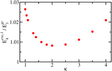
Figure 1: (color online) Energy of the four-body excited state supported by Model I at unitarity. Circles show the energy ratio $E_{4}^{\text{exc},1}/E_{3}^{\text{gr}}$ as a function of the mass ratio $\kappa$.

Table 1: Bound state energies for the B_N-1X system, $N=3-6$, with infinitely large $s$-wave scattering length $a_{\text{BX}}$ and $d_{\text{BB}}=d_{\text{BBX}}=0$ (Model I) for various mass ratios $\kappa$. Since $|E_{3}^{\text{gr}}|/E_{\text{sr}}$ (see column 2) increases with increasing $\kappa$, the results are expected to be less universal for larger $\kappa$ than for smaller $\kappa$ (see text for details). The “missing entries” correspond to parameter combinations where either the calculation was not attempted or no bound state was found. The energy ratios in columns 3-11 have uncertainties in the last digit reported.

$\kappa$	$|E_{3}^{\text{gr}}|/E_{\text{sr}}$	$E_{3}^{\text{gr}}/E_{3}^{\text{exc,1}}$	$E_{3}^{\text{exc,1}}/E_{3}^{\text{exc,2}}$	$E_{3}^{\text{exc,2}}/E_{3}^{\text{exc,3}}$	$E_{4}^{\text{gr}}/E_{3}^{\text{gr}}$	$E_{4}^{\text{exc,1}}/E_{3}^{\text{gr}}$	$E_{4}^{\text{exc,2}}/E_{3}^{\text{gr}}$	$E_{4}^{\text{exc,3}}/E_{3}^{\text{gr}}$	$E_{5}^{\text{gr}}/E_{3}^{\text{gr}}$	$E_{6}^{\text{gr}}/E_{3}^{\text{gr}}$
$1$	$2.354\times 10^{-4}$				$12.21$	$1.026$			$43.60$	$97.92$
$2$	$3.470\times 10^{-3}$	$23860.$			$6.956$	$1.008$			$18.64$	$35.20$
$3$	$9.660\times 10^{-3}$	$3398.$			$5.646$	$1.011$			$13.69$	$24.35$
$4$	$1.694\times 10^{-2}$	$1140.$			$5.046$	$1.021$			$11.61$	$20.03$
$8$	$4.437\times 10^{-2}$	$151.8$			$4.184$	$1.130$			$8.840$	$14.51$
$12$	$6.512\times 10^{-2}$	$58.52$	$66.09$		$3.892$	$1.310$			$7.964$	$12.83$
$16$	$8.082\times 10^{-2}$	$30.98$	$39.35$		$3.740$	$1.489$			$7.519$	$11.99$
$133/6$	$9.881\times 10^{-2}$	$15.47$	$23.49$	$23.67$	$3.606$	$1.711$			$7.134$	$11.27$
$26$	$1.075\times 10^{-1}$	$11.22$	$18.70$	$18.90$	$3.552$	$1.819$	$1.013$		$6.981$	$10.98$
$30$	$1.152\times 10^{-1}$	$8.575$	$15.41$	$15.64$	$3.508$	$1.911$	$1.059$		$6.859$	$10.76$
$35$	$1.232\times 10^{-1}$	$6.587$	$12.62$	$12.91$	$3.467$	$2.005$	$1.134$		$6.742$	$10.54$
$40$	$1.300\times 10^{-1}$	$5.371$	$10.66$	$11.04$	$3.434$	$2.082$	$1.214$		$6.651$	$10.37$
$45$	$1.358\times 10^{-1}$	$4.572$	$9.182$	$9.680$	$3.408$	$2.145$	$1.290$		$6.578$	$10.24$
$50$	$1.409\times 10^{-1}$	$4.016$	$8.021$	$8.648$	$3.386$	$2.199$	$1.362$	$1.003$	$6.518$	$10.13$

Table 2: Column 2 shows the scaling parameter $\lambda^{2}$ predicted by the zero-range theory for the three-body system for various $\kappa$.

$\kappa$	$\lambda^{2}$
$1$	$(1986.1)^{2}=3.9447\times 10^{6}$
$2$	$(153.84)^{2}=23666.$
$3$	$(57.876)^{2}=3349.6$
$4$	$(33.491)^{2}=1121.6$
$8$	$(12.488)^{2}=155.94$
$12$	$(8.1305)^{2}=66.105$
$16$	$(6.2804)^{2}=39.443$
$133/6$	$(4.8651)^{2}=23.670$
$26$	$(4.3477)^{2}=18.902$
$30$	$(3.9553)^{2}=15.644$
$35$	$(3.5944)^{2}=12.920$
$40$	$(3.3249)^{2}=11.055$
$45$	$(3.1152)^{2}=9.7047$
$50$	$(2.9470)^{2}=8.6847$

Table 3: Resonance energies for the B_N-1X system, $N=4$, interacting through a BX Gaussian potential with infinitely large $s$-wave scattering length $a_{\text{BX}}$ and $d_{\text{BB}}=d_{\text{BBX}}=0$ (Model I) for various mass ratios $\kappa$. Columns 2-5 report four-body resonances tied to the first excited three-body state with energy $E_{3}^{\text{exc},1}$, columns 6-7 report four-body resonances tied to the second excited three-body state with energy $E_{3}^{\text{exc},2}$, and column 8 reports four-body resonances tied to the third excited three-body state with energy $E_{3}^{\text{exc},3}$. The missing entries indicate that a calculation was either not attempted or did not yield reliable results. In some cases, we were able to determine $E_{r}$ approximately but not $E_{i}$; in these cases, the $E_{i}$ entry is marked by “?”.

$\kappa$	$\left(\frac{E_{r}}{E_{3}^{\text{exc,1}}},\frac{E_{i}}{E_{3}^{\text{exc,1}}}\right)$	$\left(\frac{E_{r}}{E_{3}^{\text{exc,1}}},\frac{E_{i}}{E_{3}^{\text{exc,1}}}\right)$	$\left(\frac{E_{r}}{E_{3}^{\text{exc,1}}},\frac{E_{i}}{E_{3}^{\text{exc,1}}}\right)$	$\left(\frac{E_{r}}{E_{3}^{\text{exc,1}}},\frac{E_{i}}{E_{3}^{\text{exc,1}}}\right)$	$\left(\frac{E_{r}}{E_{3}^{\text{exc,2}}},\frac{E_{i}}{E_{3}^{\text{exc,2}}}\right)$	$\left(\frac{E_{r}}{E_{3}^{\text{exc,2}}},\frac{E_{i}}{E_{3}^{\text{exc,2}}}\right)$	$\left(\frac{E_{r}}{E_{3}^{\text{exc,3}}},\frac{E_{i}}{E_{3}^{\text{exc,3}}}\right)$
$4$	$(3.28,\approx 0.03)$
$8$	$(2.63,0.018)$
$12$	$(2.35,0.019)$
$16$	$(2.19,0.011)$				$(2.22,\approx 0.01)$
$133/6$	$(2.19,0.009)$	$(1.03,0.004)$			$(2.08,0.020)$		$(1.96,?)$
$26$	$(2.45,0.023)$	$(1.19,0.028)$			$(2.05,0.016)$
$30$	$(2.95,0.047)$	$(1.44,0.047)$			$(2.06,0.005)$	$(1.04,0.003)$	$(2.00,?)$
$35$	$(3.46,0.048)$	$(1.61,0.055)$			$(1.93,0.003)$	$(1.03,0.0006)$
$40$	$(3.73,0.039)$	$(1.73,0.056)$	$(1.02,0.010)$		$(\approx 1.94,?)$	$(\approx 1.03,?)$	$(\approx 2.01,?)$
$45$	$(3.85,0.030)$	$(1.83,0.051)$	$(1.20,0.0009)$	$(1.04,0.015)$	$(1.86,0.078)$	$(1.04,?)$	$(2.07,?)$
$50$	$(3.90,0.026)$	$(1.94,0.049)$	$(1.46,?)$	$(1.10,0.021)$	$(1.85,?)$	$(1.03,?)$	$(2.40,\approx 0.036)$

Analysis of the four-body resonance states that are tied to $E_{3}^{\text{exc},j}$ shows, as we will discuss now, that the four-body spectra reported in Table 1, especially for large $\kappa$, are not universal; this is, of course, not surprising given the discussion presented in Sec. II. Table 3 summarizes the real and imaginary parts $E_{r}$ and $E_{i}$ of the four-body resonance energies for $\kappa=4-50$. In Table 3, $E_{r}$ and $E_{i}$ are reported in terms of the excited three-body bound state energies $E_{3}^{\text{exc},j}$. As mentioned in Appendix A, a precise and unambiguous identification of resonance states becomes numerically more challenging as $|E_{r}|/E_{\text{sr}}$ and/or $|E_{i}|/E_{\text{sr}}$ decrease. Consequently, Table 3 reports results for resonances tied to three different three-body states for $\kappa=50$ but only one three-body state for $\kappa=4$. For $\kappa\leq 4$, the complex scaling approach, as implemented by us, did not yield reliable four-body results.

We first discuss our results for $\kappa=4-16$. For these $\kappa$, the ratio $E_{r}/E_{3}^{\text{exc},1}$ deviates notably from both the energy ratios $E_{4}^{\text{gr}}/E_{3}^{\text{gr}}$ and $E_{4}^{\text{exc,1}}/E_{3}^{\text{gr}}$, indicating that the four-body results reported in Table 1 are not universal. For $\kappa=16$, we were able to reliably determine $E_{r}$ for a four-body resonance tied to the second excited trimer state, yielding $E_{r}/E_{3}^{\text{exc,2}}=2.22$. Since this value is close to the ratio of $2.19$ obtained for the resonance attached to the first excited trimer, we conclude that the energy ratios for the four-body resonances for $\kappa=4-16$, tied to the first excited three-body state, are close to universal.

For larger mass ratios, the four-body resonances tied to the first excited trimer are not universal. However, closer to universal results are obtained for the resonances that are tied to the second or third excited trimers. For $\kappa=30-50$, our complex scaling results suggest that there are two four-body states tied to each Efimov trimer, with the second state having a resonance position that is just a bit below the corresponding trimer energy. For smaller $\kappa$, “excited” four-body resonance states with real parts $E_{r}$ very close to the Efimov trimer energy may also exist. However, we were not able to describe such resonance states by our approach. We note that the identification of the four-body resonances for $\kappa\gtrsim 35$ is challenging due to the existence of multiple four-body resonances. For $\kappa=35$, e.g., we find a resonance at $E_{r}\approx 4.9E_{3}^{\text{exc},2}$ that is not reported in Table 3 since we believe that this resonance would not “survive” if we went to resonances that are attached to more highly-excited three-body states.

Importantly, the complex scaling calculations also provide estimates of the lifetimes $\tau$. If expressed, as in Table 3, in terms of the corresponding trimer energies, the imaginary parts $E_{i}$ of the resonance energies are comparable, in terms of the order of magnitude, to those found for the equal-mass four-boson system. For example, Ref. Deltuva2 found $E_{r}=4.6108E_{3}^{\text{exc},j}$ and $E_{i}=0.01484E_{3}^{\text{exc},j}$ for the energetically lower-lying BBBB state and $E_{r}=1.00228E_{3}^{\text{exc},j}$ and $E_{i}=2.38\times 10^{-4}E_{3}^{\text{exc},j}$ for the energetically higher-lying BBBB state in the large $j$ limit. This suggests that signatures of the four-body resonance states of unequal-mass systems should be observable experimentally.

III.2 Model II

Since resonance states are, in general, more challenging to determine than bound states, it is desirable to employ an interaction model for which the ground state of the trimer behaves close to universal. This section summarizes our energies at unitarity for Model II, for which the repulsive BBX potential leads to a significant reduction of the binding energy of the ground state trimer. Table 4 summarizes three-, four-, and five-body energies, which are obtained for such a large $d_{\text{BBX}}$ that the difference to the infinity limit is rather small (see also Ref. BlumeYanPRL ). In general, the resulting energy ratios could depend on the details of the underlying potential model. For the three-body sector, we believe that the results reported in Table 4 are, to a very good approximation, universal since $E_{3}^{\text{gr}}/E_{3}^{\text{exc,1}}$ is close to the zero-range prediction for $\lambda^{2}$.

As discussed in Ref. BlumeYanPRL , the four-body systems with $\kappa\geq 16$ support two four-body states. One four-body state is roughly twice as strongly bound as the trimer while the other is extremely weakly bound. As the mass ratio decreases, the weakly-bound state disappears (or at least our calculations were not able to describe it) while the deeper-lying four-body state becomes more strongly bound. For $\kappa=1$, e.g., the binding energy of the ground state tetramer is roughly 10 times larger than that of the ground state trimer. In terms of size, this suggests that the ground state tetramer is smaller by about a factor of $\sqrt{10}$ than the ground state trimer. Since $|E_{4}^{\text{gr}}|/E_{\text{sr}}$ is still much smaller than 1, we believe that the tetramer energy is close to universal. This is confirmed by the fact that Refs. PRXMonash ; GiorginiPRA1 found similar ratios for $E_{4}^{\text{gr}}/E_{3}^{\text{gr}}$, namely $9.35-9.7$, using different models. We note that the energy ratio $E_{4}^{\text{gr}}/E_{3}^{\text{gr}}$ of $9.74$ (see Table 4) for the $\kappa=1$ system with large repulsive three-body force is about 20 % smaller than the energy ratio $E_{4}^{\text{gr}}/E_{3}^{\text{gr}}$ of $12.21$ obtained in the absence of the three-body force (see Table 1). This indicates that the $\kappa=1$ results reported in Table 1 are not universal despite the fact that the ratio $|E_{3}^{\text{gr}}|/E_{\text{sr}}$ is rather small.

Interestingly, Ref. PRXMonash reported the existence of an extremely weakly-bound excited four-body state for $\kappa=1$ (see Table I of Ref. PRXMonash ). For our Model II, we were not able to find such a state. Looking ahead, we note that our calculations for Model III with large $d_{\text{BX}}$ suggest, in agreement with Table 4, that the $\kappa=1$ and $12$ systems do not support an excited four-body state at unitarity. While we cannot rule out that this is due to the variational character of our calculations (i.e., an excited state is supported by Model II but we missed it), we speculate that the disagreement between our results and Ref. PRXMonash points toward a sensitive dependence of the energy ratios on the underlying model interaction.

Table 4 also reports five-body energies. These will be discussed in more detail in the next section.

Table 4: Energies of the B_N-1X system, $N=3-4$, interacting through a BX Gaussian potential with infinitely large $s$-wave scattering length $a_{\text{BX}}$, repulsive three-body Gaussian potential, and vanishing BB potential ($d_{\text{BB}}=0$) for various mass ratios (Model II). The $\kappa=1$, $2$, and $4$ energies are obtained for $d_{\text{BBX}}=4.8E_{\text{sr}}$; the reported energies should be close to the $d_{\text{BBX}}\rightarrow\infty$ limit. We find $|E_{3}^{\text{gr}}|/E_{\text{sr}}=2.4\times 10^{-8}$, $3.1\times 10^{-6}$, and $4.6\times 10^{-5}$ for $\kappa=1$, $2$, and $4$, respectively. The entry “$-$” indicates that a bound state was not found. The energies for $\kappa=8-50$ are taken from Ref. BlumeYanPRL .

$\kappa$	$E_{3}^{\text{gr}}/E_{3}^{\text{exc,1}}$	$E_{4}^{\text{gr}}/E_{3}^{\text{gr}}$	$E_{4}^{\text{exc,1}}/E_{3}^{\text{gr}}$	$E_{5}^{\text{gr}}/E_{3}^{\text{gr}}$
$1$		$9.51$	$-$	$25.1$
$2$		$4.85$	$-$	$9.74$
$4$		$3.36$	$-$	$5.71$
$8$	$(12.510)^{2}\approx 156.5$	$(1.647)^{2}\approx 2.713$	$-$	$(2.06)^{2}\approx 4.244$
$12$	$(8.158)^{2}\approx 66.55$	$(1.58)^{2}\approx 2.496$	$-$	$(1.94)^{2}\approx 3.764$
$16$	$(6.313)^{2}\approx 39.85$	$(1.544)^{2}\approx 2.384$	$(1.002)^{2}\approx 1.004$	$(1.88)^{2}\approx 3.534$
$133/6$	$(4.904)^{2}\approx 24.05$	$(1.510)^{2}\approx 2.280$	$(1.010)^{2}\approx 1.020$	$(1.82)^{2}\approx 3.312$
$30$	$(3.998)^{2}\approx 15.98$	$(1.488)^{2}\approx 2.214$	$(1.026)^{2}\approx 1.053$	$(1.78)^{2}\approx 3.168$
$40$	$(3.372)^{2}\approx 11.37$	$(1.471)^{2}\approx 2.164$	$(1.046)^{2}\approx 1.094$	$(1.75)^{2}\approx 3.063$
$50$	$(2.996)^{2}\approx 8.714$	$(1.461)^{2}\approx 2.135$	$(1.067)^{2}\approx 1.138$	$(1.73)^{2}\approx 2.993$

III.3 Model III

Reference GiorginiPRA1 investigated the equal-mass polaron problem by modeling the boson-boson interaction by a repulsive two-body step potential. It was later argued PRXMonash that the results for the interaction model used in Ref. GiorginiPRA1 (basically, our Model III with repulsive and attractive two-body step potentials instead of repulsive and attractive two-body Gaussian potentials) should be universal, provided the energies are scaled by the trimer ground state energy. Interestingly, Ref. GiorginiPRA1 found four- and five-body bound states but no six-body bound state. It was suggested PRXMonash that this may be due to the fact that a single impurity can bind one $s$- and three $p$-wave bosons and that shell closure prevents the binding of additional bosons. In the following, the question of universality and the existence of six-body bound states is investigated using Model III.

Circles in Figs. 2(a) and 2(b) show the energy ratio $E_{3}^{\text{gr}}/E_{3}^{\text{exc},1}$ as a function of $a_{\text{BB}}/r_{\text{BB}}$ for $\kappa=12$ and $\kappa=133/6$, respectively. For comparison, the horizontal dashed lines show the scaling parameter $\lambda^{2}$ from the zero-range theory, which assumes vanishing BB interactions. The energy ratios for Model III plateau as $a_{\text{BB}}/r_{\text{BB}}$ increases at a value somewhat larger than that predicted by the zero-range theory. The deviation between $E_{3}^{\text{gr}}/E_{3}^{\text{exc},1}$ for the largest $a_{\text{BB}}$ considered and the zero-range scaling parameter is 0.19 % and 1.4 % for $\kappa=12$ and $\kappa=133/6$, respectively. This shows that the actual value of the $a_{\text{BB}}$ scattering length plays a secondary role, provided $a_{\text{BB}}$ is much smaller than the size of the ground state trimer. A sufficiently large positive value of $a_{\text{BB}}$ leads to the exclusion of a portion of the configuration space, thereby bringing the results closer to the universal regime. We were unfortunately not able to reliably determine $E_{3}^{\text{exc},1}$ for $\kappa=1$ due to the extremely large scaling parameter. We expect that $E_{3}^{\text{gr}}/E_{3}^{\text{exc},1}$ would reach a plateau for smaller $a_{\text{BB}}/r_{\text{BB}}$ than for $\kappa=12$ and that the percentage deviation between the plateau value and the zero-range scaling parameter would be smaller than the percentage deviation for $\kappa=12$.

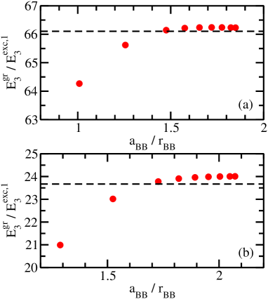
Figure 2: (color online) Characteristics of Model III at unitarity. Circles show the energy ratio $E_{3}^{\text{gr}}/E_{3}^{\text{exc},1}$ as a function of $a_{\text{BB}}/r_{\text{BB}}$ for (a) $\kappa=12$ and (b) $\kappa=133/6$. For comparison, dashed horizontal lines show the zero-range scaling parameter $\lambda^{2}$ from Table 2.

Figures 3(a)-3(c) summarize our $N=4-6$ results for $\kappa=1$, $\kappa=12$, and $\kappa=133/6$, respectively. For all three mass ratios, the change of $E_{N}^{\text{gr}}/E_{3}^{\text{gr}}$ decreases with increasing $a_{\text{BB}}/r_{\text{BB}}$. For fixed mass ratio $\kappa$, the energy ratio $E_{4}^{\text{gr}}/E_{3}^{\text{gr}}$ (circles) reaches a plateau quicker than the energy ratios $E_{5}^{\text{gr}}/E_{3}^{\text{gr}}$ (squares) and $E_{6}^{\text{gr}}/E_{3}^{\text{gr}}$ (triangles). Also, the “flattening” with increasing $a_{\text{BB}}/r_{\text{BB}}$ is faster for $\kappa=1$ than for $\kappa=12$ and $133/6$. For comparison, the dashed horizontal lines on the right edge of Figs. 3(a)-3(c) show the energy ratios for Model II (see Table 4 and Ref. BlumeYanPRL ). For $N=4$, the energy ratios for Model III (circles) for the largest $a_{\text{BB}}/r_{\text{BB}}$ considered and Model II (lowest dashed line) differ by about 2.4 %, 7.1 %, and 3.9 % for $\kappa=1$, $12$, and $133/6$, respectively. The calculations underline that it is challenging to reach the fully universal regime for large mass ratios by adding purely repulsive two- or three-body potentials. The deviations for $N=5$ are $0$ %, 19 %, and 13 % for $\kappa=1$, $12$, and $133/6$, respectively. Generally speaking, we expect that the discrepancy between the two sets of results would increase with increasing $N$. For $\kappa=133/6$, this is indeed the case [see Fig. 3(c)]. For $N=6$ and $\kappa=1$, Fig. 3(a) shows converged energy ratios up to $a_{\text{BB}}/r_{\text{BB}}\approx 0.285$; for larger $a_{\text{BB}}/r_{\text{BB}}$, our energy ratios (not shown) are not fully converged. For $a_{\text{BB}}/r_{\text{BB}}\approx 0.6$, e.g., we find $E_{6}^{\text{gr}}/E_{3}^{\text{gr}}=35.2$, which should be considered as a lower bound since our calculations are variational and $E_{3}^{\text{gr}}$ is highly accurate. We conclude that Model III suports a six-body bound state in the large $d_{\text{BBX}}$ limit. Such a bound state was not found in Ref. GiorginiPRA1 for the square-well model. This suggests that the shell-closure argument put forward in Ref. PRXMonash does not hold, in general, for bosonic systems with an impurity. The discussion surrounding Fig. 3 can be summarized as follows: While Models II and III predict somewhat different energy ratios for $N\geq 5$, we believe that these models provide a realistic description of the hierarchy of few-body states of small bosonic systems with a single impurity.

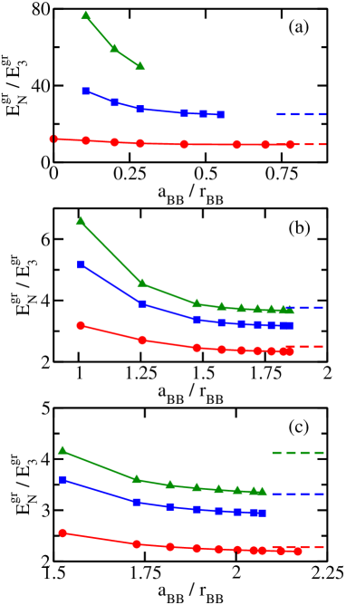
Figure 3: (color online) Comparison of ground state energies for Models II and III at unitarity. Circles, squares, and triangles show the energy ratios $E_{4}^{\text{gr}}/E_{3}^{\text{gr}}$, $E_{5}^{\text{gr}}/E_{3}^{\text{gr}}$, and $E_{6}^{\text{gr}}/E_{3}^{\text{gr}}$, respectively, as a function of $a_{\text{BB}}/r_{\text{BB}}$ for (a) $\kappa=1$, (b) $\kappa=12$, and (c) $\kappa=133/6$ for Model III; the lines connecting the symbols serve as a guide to the eye. The dashed horizontal lines show the energy ratios for Model II (see Table 4). The $N=6$ energy ratio for Model II is only shown for $\kappa=133/6$.

Reference BlumeYanPRL (see also Table 4) found that Model II at unitarity supports an excited four-body state for $\kappa=16-50$. For $\kappa=12$, in contrast, no such state was found. The corresponding results for Model III are summarized in Fig. 4. The change of the energy ratio $E_{4}^{\text{exc},1}/E_{3}^{\text{gr}}$ decreases as $a_{\text{BB}}/r_{\text{BB}}$ increases. For the largest $a_{\text{BB}}/r_{\text{BB}}$ considered, the energy ratio $E_{4}^{\text{exc},1}/E_{3}^{\text{gr}}$ for $\kappa=133/6$ takes a value of around $1.011$, which is somewhat smaller, accounting for error bars, than the corresponding value of $1.020$ for Model 2 (according to Ref. BlumeYanPRL , the errorbar is $0.005$ on the square root of the energy ratio).

In agreement with the Model II results, we find that the excited four-body state for $\kappa=12$ disappears as $a_{\text{BB}}/r_{\text{BB}}$ goes beyond a critical value [$a_{\text{BB}}/r_{\text{BB}}\gtrsim 1.42$; see Fig. 4(a)], which is smaller than the value for which we would expect, based on the ground state results shown in Fig. 3, the energy ratio to be independent of $a_{\text{BB}}/r_{\text{BB}}$. Figure 4 indicates that the predictions of Models II and III for the energy ratio $E_{4}^{\text{exc},1}/E_{3}^{\text{gr}}$ are reasonably consistent.

For $\kappa=1$, we find that the excited four-body state supported by Model I disappears when the boson-boson scattering length is sufficiently repulsive (Model III). The absense of an excited four-body state at unitarity for $\kappa=1$, as predicted by Models II and III, is in disagreement with the predictions of the “$r_{0}$ and $\Lambda$ models” of Ref. PRXMonash . In those models, an energy for the excited four-body state, expressed in terms of the three-body ground state energy, of $1.0030(3)$ and $1.0036(1)$ was reported for the $r_{0}$ and $\Lambda$ models, respectively. Since the binding energy is extremely small, it might be that a small change in the interaction model moves the critical scattering length of the excited four-body state from the positive to the negative scattering length side, thereby explaining the discrepancy. Alternatively, it could be that our model supports an excited four-body bound state at unitarity but that our numerical approach missed the state.

Figure 4: (color online) Energies of the excited four-body states at unitarity. Circles show the energy ratio $E_{4}^{\text{exc},1}/E_{3}^{\text{gr}}$ for Model III as a function of $a_{\text{BB}}/r_{\text{BB}}$ for (a) $\kappa=12$ and (b) $\kappa=133/6$; the lines connecting the symbols serve as a guide to the eye. The horizontal dashed line in panel (b) shows the corresponding energy ratio for Model II.

IV Results: Negative scattering length side

This section discusses the behavior of the BBBX system with $\kappa=133/6$ as a function of the interspecies $s$-wave scattering length $a_{\text{BX}}$ ($a_{\text{BX}}<0$). For Model II, the critical BX scattering lengths $a_{4,-}^{\text{gr}}$ and $a_{4,-}^{\text{exc,1}}$, at which the ground and first excited tetramer energies are resonant with the four-atom threshold, were predicted to be $a_{4,-}^{\text{gr}}\approx 0.55a_{3,-}$ and $a_{4,-}^{\text{exc}}\approx 0.91a_{3,-}$, respectively BlumeYanPRL . Here, $a_{3,-}$ is the critical BX scattering length at which the trimer that the four-body states are tied to becomes unbound on the negative scattering length side.

To obtain a sense for the dependence of these results on the underlying model, we additionally performed calculations for the negative $a_{\text{BX}}$ regime using Model I. Specifically, we determine the energy of the four-body resonances tied to the first excited BBX trimer. The results are summarized in Fig. 5. The solid line shows the energy $E_{3}^{\text{exc},1}$ of the first excited trimer while the circles and squares show the real part $E_{r}$ of the energetically lower- and higher-lying four-body resonances. The absolute value $|E_{i}|$ of the imaginary part is shown by errorbars. For example, the magnitude of the imaginary part $E_{i}$ of the resonance energy of the energetically lower-lying four-body state changes from $9\times 10^{-3}E_{3}^{\text{exc},1}$ at unitarity to around $10^{-4}E_{3}^{\text{exc},1}$ for the point closest to threshold in Fig. 5. The magnitude of the imaginary part $E_{i}$ of the resonance energy of the energetically higher-lying four-body state changes from $4\times 10^{-3}E_{3}^{\text{exc},1}$ at unitarity to around $2\times 10^{-4}E_{3}^{\text{exc},1}$ for the point closest to threshold in Fig. 5. Extrapolating the four-body resonance energies $E_{r}$ to zero, we estimate the following critical scattering lengths for the two four-body states: $a_{4,-}^{\text{gr}}\approx 0.66a_{3,-}$ and $a_{4,-}^{\text{exc,1}}\approx 0.94a_{3,-}$. The agreement with the results for Model II is quite good, especially considering that the critical scattering lengths have a few percent uncertainty due to numerical inaccuracies and that the determination of the critical scattering lengths requires an extrapolation to the threshold.

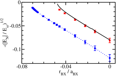
Figure 5: (color online) Generalized Efimov spectrum, obtained using Model I, for $\kappa=133/6$ as a function of the inverse of the BX $s$-wave scattering length $a_{\text{BX}}$ (only the negative $a_{\text{BX}}$ regime is shown). The energies and scattering lengths are scaled by the short-range quantities $E_{\text{sr}}$ and $r_{\text{BX}}$, respectively (the energy is shown on a square-root scale). The solid line shows the energy $E_{3}^{\text{exc},1}$ of the BBX system. The circles and squares show the real part $E_{r}$ of the resonance energies of the BBBX system (to guide the eye, the dotted line connects consecutive points for the energetically lower-lying resonance). The error bars indicate the absolute value of the imaginary part $E_{i}$ of the resonance energy (again, using the square-root scaling); a smaller $|E_{i}|/E_{\text{sr}}$ corresponds to a larger scaled lifetime.

V Summarizing remarks

This work determined the bound state energies of an impurity that interacts with $N-1$ bosonic atoms through short-range interactions that are characterized by the $s$-wave scattering length $a_{\text{BX}}$. For the cases considered, the impurity mass was the same as or smaller than that of the bosons. Impurity problems are ubiquitous in physics, ranging from impurities in condensed matter systems to impurities in quantum liquid droplets, such as helium and molecular hydrogen clusters, to impurities in cold fermionic and bosonic atomic gases. A key objective of the present work was to investigate, using two-body interactions that mimick zero-range interactions in the limit that the trimer size is large compared to the range of the two-body potential, universal four- and higher-body states that are linked to three-body Efimov trimers consisting of two bosonic atoms and the impurity. To address this objective, the results for different interaction models were compared. While the present work considered two-body single-channel models, Ref. PRXMonash treated the $N=4$ system with $\kappa=1$ using a two-body coupled-channel model.

The impurity problem studied in this work is unique due to its close connection to three-body Efimov states. In the large $|a_{\text{BX}}|$ limit, the weakly-bound BBX states follow Efimov’s radial scaling law, which implies that the three-body states are governed by the $s$-wave scattering length and a three-body parameter. If the four-body states are fully governed by these parameters, then different interaction models should, in the limit that the effective range corrections can be neglected, yield the same value for the four-body energies, provided the four-body energies are expressed in terms of the three-body energy and provided the $s$-wave scattering lengths are the same. This work shows that this is the case for $N=4$ and $\kappa=1$. As the mass ratio $\kappa$ increases, model dependencies at the few percent level develop. For the five-body system, the energy ratio $E_{5}^{\text{gr}}/E_{3}^{\text{gr}}$ displays, for $\kappa=12$ and $133/6$, a stronger model dependence than the energy ratio $E_{4}^{\text{gr}}/E_{3}^{\text{gr}}$. In general, the “universality window” decreases with increasing number of particles since the binding energy increases (i.e., the system size shrinks with increasing $N$). This is particularly prominent when $\kappa$ is notably larger than $1$. It would be interesting to extend the very recent effective field theory study for identical bosons EFT to the bosonic system with impurity considered in this work. Specifically, it would be interesting to explore at which order the four-body parameter enters. It should be kept in mind that the numerical calculations become more challenging as $N$ increases, implying that it is harder to exhaustively explore the parameter space of the model interactions with high accuracy for $N=5$ and $N=6$. Model III suggests, in contrast to what was found in Ref. GiorginiPRA1 for a slightly different model, that the system for $\kappa=1$ supports a six-body bound state. It will be interesting to explore the implications of this bound state on the physics of the Bose polaron.

VI Acknowledgement

Support by the National Science Foundation through grant number PHY-1806259 is gratefully acknowledged.

Appendix A Illustration of complex scaling approach

This appendix illustrates the complex scaling approach, using a basis set constructed from explicitly correlated Gaussian basis functions, for the BBBX system with mass ratio $\kappa=8$ for infinitely large BX scattering length, $d_{\text{BB}}=d_{\text{BBX}}=0$ (Model I), and $E_{\text{target}}=-2.52\times 10^{-4}E_{\text{sr}}$. This target energy is about three times less negative than the resonance energy of $E_{r}=-7.69\times 10^{-4}E_{\text{sr}}$ reported in Table 3.

To illustrate the construction of the basis set, Fig. 6 shows the eigen values as a function of the inverse of the number $N_{b}$ of basis functions. For the example at hand, the first 100 basis functions were chosen such that the two bound four-body states (see Table 1) are reasonably well described. For $N_{b}=250$ (right edge of the figure), the state with energy larger than and closest to the target energy corresponds to the 8-th eigen value. As more basis functions are added, the energy of the 8-th state drops below $E_{\text{target}}$ (this occurs around $1/N_{b}=0.0035$ in Fig. 6) and the next higher-lying state is being optimized. This “dropping down” is repeated several times during the optimization procedure. The reason that the energy “drops” during the optimization is that there exists a continuum of “trimer-plus-atom states” above the three-body ground state. Since the basis functions have a finite as opposed to an infinite spatial extend and since the basis set is finite, the continuum is discretized. The roughly flat portion (plateau at $E_{4}\approx-7.7\times 10^{-4}E_{\text{sr}}$) of the eigen values is, as confirmed by the results presented in Fig. 7, associated with a resonance state.

To extract quantitative information, we solve the eigen value problem spanned by $\tilde{\underline{H}}_{\text{rel}}$ and $\underline{O}$ for various $\theta$. The resulting eigen values are categorized as corresponding to bound states, scattering states, and resonance states according to the behavior of the trajectories in the complex plane. To locate the resonance states, we plot the trajectories, which span several orders of magnitude in $E_{r}$ and $E_{i}$, in different energy windows. Squares, circles, triangles, and diamonds in Fig. 7 show trajectories corresponding to a resonance state using basis sets with $N_{b}=1600$, $2000$, $2500$, and $3000$ (the same basis functions as used in Fig. 6). The “beginning point” ($\theta=0$) of the trajectories can be identified by the condition that the imaginary part of the energy is zero for $\theta=0$. For each trajectory, the symbols are obtained for equally spaced $\theta$. It can be seen that the trajectories for the different basis set sizes all go, roughly, through the point $(E_{r},E_{i})\approx(-7.69\times 10^{-4}E_{\text{sr}},-5.3\times 10^{-6}E_{\text{sr}})$. Moreover, at or near this point in the complex energy plane, the trajectories for $N_{b}=2000$, $2500$, and $3000$ slow down; this can be seen from the decreased spacing of the symbols. For the example shown, the calculations for $N_{b}=1600$ do not allow us to extract the resonance energy and lifetime. It is ensuring, though, that the results for $N_{b}=2000-3000$ agree with each other. Repeating the calculations for different $E_{\text{target}}$ to ensure independence of $E_{\text{target}}$, we extract the resonance position and its lifetime. The resonance energy moves somewhat for different $E_{\text{target}}$ and different basis sets. The results reported in Table 3 are, in most cases, averages from multiple runs.

In general, we find that the resonance position (i.e., the real part $E_{r}$) is numerically more stable than the lifetime $\tau$ [which is proportional to the inverse of the imaginary part, $\tau=h/(2|E_{i}|)$]. Also, as a rule of thumb, the closer the real part $E_{r}$ is to zero, the harder it is to reliably extract the lifetime from our calculations. Because of this, our complex scaling calculations (see Table 3) are restricted to mass ratios $\kappa\geq 4$).

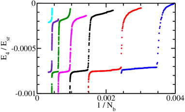
Figure 6: (color online) Basis set generation for BBBX system with infinitely large interspecies $s$-wave scattering length and $\kappa=8$ (Model I). The target energy $E_{\text{target}}$ is set to $-2.52\times 10^{-4}E_{\text{sr}}$. The symbols show the four-body energies $E_{4}$ as a function of the inverse of the number $N_{b}$ of basis functions. The displayed energies correspond to the 8-th through 14-th eigen value of the generalized eigen value problem. The “plateau” at $E_{4}\approx-7.8\times 10^{-4}E_{\text{sr}}$ is indicative of a four-body resonance (see also Fig. 7). The data suggest that there may exist another resonance at $E_{r}\approx-2\times 10^{-4}E_{\text{sr}}$. However, the complex scaling did not reveal such a resonance. This is likely due to the fact that the energetically higher-lying plateau is not a signature of a resonance but related to a BBX bound state.

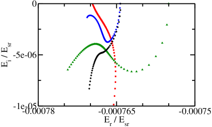
Figure 7: (color online) Complex scaling results for the BBBX system with infinitely large interspecies $s$-wave scattering length and $\kappa=8$ (Model I). Red squares, blue circles, green triangles, and black diamonds show trajectories, generated by scanning the rotation angle $\theta$, in the complex energy plane for $N_{b}=1600$, $2000$, $2500$, and $3000$, respectively ($\theta$ is increased linearly in steps of approximately $6.957\times 10^{-3}$radians for $N_{b}=1600$, $8.276\times 10^{-3}$radians for $N_{b}=2000$, $6.667\times 10^{-3}$radians for $N_{b}=2500$, and $8.421\times 10^{-3}$radians for $N_{b}=3000$). For vanishing rotation angle, the imaginary part of the energy is zero. This figure and Fig. 6 are obtained using the same basis set.

References

- (1) M. Greiner, O. Mandel, T. Esslinger, T. W. Hänsch, and I. Bloch, Quantum phase transition from a superfluid to a Mott insulator in a gas of ultracold atoms, Nature 415, 39 (2002).
- (2) M. R. Matthews, B. P. Anderson, P. C. Haljan, D. S. Hall, C. E. Wieman, and E. A. Cornell, Vortices in a Bose-Einstein Condensate, Phys. Rev. Lett. 83, 2498 (1999).
- (3) J. R. Abo-Shaeer, C. Raman, J. M. Vogels, and W. Ketterle, Observation of Vortex Lattices in Bose-Einstein Condensates, Science 292, 476 (2001).
- (4) A. Schirotzek, C.-H. Wu, A. Sommer, and M. W. Zwierlein, Observation of Fermi Polarons in a Tunable Fermi Liquid of Ultracold Atoms, Phys. Rev. Lett. 102, 230402 (2009).
- (5) N. Navon, S. Nascimbène, F. Chevy, and C. Salomon, The Equation of State of a Low-Temperature Fermi Gas with Tunable Interactions, Science 328, 729 (2010).
- (6) C. Kohstall, M. Zaccanti, M. Jag, A. Trenkwalder, P. Massignan, G. M. Bruun, F. Schreck, and R. Grimm, Metastability and coherence of repulsive polarons in a strongly interacting Fermi mixture, Nature 485, 618 (2012).
- (7) M.-G. Hu, M. J. Van de Graaff, D. Kedar, J. P. Corson, E. A. Cornell, and D. S. Jin, Bose Polarons in the Strongly Interacting Regime, Phys. Rev. Lett. 117, 055301 (2016).
- (8) N. B. Jørgensen, L. Wacker, K. T. Skalmstang, M. M. Parish, J. Levinsen, R. S. Christensen, G. M. Bruun, and J. J. Arlt, Observation of Attractive and Repulsive Polarons in a Bose-Einstein Condensate, Phys. Rev. Lett. 117, 055302 (2016).
- (9) P. Massignan, M. Zaccanti, and G. M. Bruun, Polarons, dressed molecules and itinerant ferromagnetism in ultracold Fermi gases, Rep. Prog. Phys. 77, 034401 (2014).
- (10) F. Chevy and C. Mora, Ultracold Polarized Fermi Gas, Rep. Prog. Phys. 73, 112401 (2010).
- (11) J. Levinsen, M. M. Parish, and G. M. Bruun, Impurity in a Bose-Einstein Condensate and the Efimov Effect, Phys. Rev. Lett. 115, 125302 (2015).
- (12) S. M. Yoshida, S. Endo, J. Levinsen, and M. M. Parish, Universality of an Impurity in a Bose-Einstein Condensate, Phys. Rev. X 8, 011024 (2018).
- (13) H.-W. Hammer and L. Platter, Universal properties of the four-body system with large scattering length, Eur. Phys. J. A 32, 113 (2007).
- (14) J. von Stecher, J. P. D’Incao, and C. H. Greene, Signatures of universal four-body phenomena and their relation to the Efimov effect, Nat. Phys. 5, 417 (2009).
- (15) A. Deltuva, Shallow Efimov tetramer as inelastic virtual state and resonant enhancement of the atom-trimer relaxation, Europhys. Lett. 95, 43002 (2011).
- (16) A. Deltuva, Efimov physics in bosonic atom-trimer scattering, Phys. Rev. A 82, 040701(R) (2010).
- (17) J. von Stecher, Five- and Six-Body Resonances Tied to an Efimov Trimer, Phys. Rev. Lett. 107, 200402 (2011).
- (18) F. Ferlaino, S. Knoop, M. Berninger, W. Harm, J. P. D’Incao, H.-C. Nägerl, and R. Grimm, Evidence for universal four-body states tied to an Efimov trimer, Phys. Rev. Lett. 102, 140401 (2009).
- (19) F. Ferlaino, A. Zenesini, M. Berninger, B. Huang, H.-C. Nägerl, and R. Grimm, Efimov Resonances in Ultracold Quantum Gases, Few-Body Syst. 51, 113 (2011).
- (20) S. E. Pollack, D. Dries, and R. G. Hulet, Universality in Three- and Four-Body Bound States of Ultracold Atoms, Science 326, 1683 (2009).
- (21) J. von Stecher, Weakly bound cluster states of Efimov character, J. Phys. B 43, 101002 (2010).
- (22) M. Gattobigio, A. Kievsky, and M. Viviani, Spectra of helium clusters with up to six atoms using soft-core potentials, Phys. Rev. A 84, 052503 (2011).
- (23) Y. Yan and D. Blume, Energy and structural properties of -boson clusters attached to three-body Efimov states: Two-body zero-range interactions and the role of the three-body regulator, Phys. Rev. A 92, 033626 (2015).
- (24) S. K. Adhikari and A. C. Fonseca, Four-body Efimov effect in a Born-Oppenheimer model, Phys. Rev. D 24, 416 (1981).
- (25) D. Blume and Y. Yan, Generalized Efimov Scenario for Heavy-Light Mixtures, Phys. Rev. Lett. 113, 213201 (2014).
- (26) Y. Wang, W. B. Laing, J. von Stecher, and B. D. Esry, Efimov Physics in Heteronuclear Four-Body Systems, Phys. Rev. Lett. 108, 073201 (2012).
- (27) L. A. Peña Ardila and S. Giorgini, Impurity in a Bose-Einstein condensate: Study of the attractive and repulsive branch using quantum Monte Carlo methods, Phys. Rev. A 92, 033612 (2015).
- (28) F. Wang, X. Ye, M. Guo, D. Blume, and D. Wang, Exploring Few-Body Processes with an Ultracold Light-Heavy Bose-Bose Mixture, arXiv:1611.03198.
- (29) C. H. Schmickler, H.-W. Hammer, and E. Hiyama, Tetramer bound states in heteronuclear systems, Phys. Rev. A 95, 052710 (2017).
- (30) P. Naidon, Tetramers of Two Heavy and Two Light Bosons, Few-Body Systems 59, 64 (2018).
- (31) S. M. Yoshida, Z.-Y. Shi, J. Levinsen, and M. M. Parish, Few-body states of bosons interacting with a heavy quantum impurity, arXiv:1807.09992.
- (32) Z.-Y. Shi, S. M. Yoshida, M. M. Parish, and J. Levinsen, Impurity-induced multi-body resonances in a Bose gas, arXiv:1807.09948.
- (33) V. N. Efimov, Weakly-bound States Of 3 Resonantly-interacting Particles, Yad. Fiz. 12, 1080 (1970); Sov. J. Nucl. Phys. 12, 589 (1971).
- (34) V. Efimov, JETP Lett. 16, 34 (1972).
- (35) V. Efimov, Energy levels of three resonantly interacting particles, Nucl. Phys. A 210, 157 (1973).
- (36) E. Braaten and H.-W. Hammer, Universality in few-body systems with large scattering length, Phys. Rep. 428, 259 (2006).
- (37) M. Berninger, A. Zenesini, B. Huang, W. Harm, H.-C. Nägerl, F. Ferlaino, R. Grimm, P. S. Julienne, and J. M. Hutson, Universality of the Three-Body Parameter for Efimov States in Ultracold Cesium, Phys. Rev. Lett. 107, 120401 (2011).
- (38) J. Wang, J. P. D’Incao, B. D. Esry, and C. H. Greene, Origin of the Three-Body Parameter Universality in Efimov Physics, Phys. Rev. Lett. 108, 263001 (2012).
- (39) P. Naidon, S. Endo, and M. Ueda, Microscopic Origin and Universality Classes of the Efimov Three-Body Parameter Phys. Rev. Lett. 112, 105301 (2014).
- (40) P. Naidon, S. Endo, and M. Ueda, Physical origin of the universal three-body parameter in atomic Efimov physics, Phys. Rev. A 90, 022106 (2014).
- (41) L. A. Peña Ardila and S. Giorgini, Bose polaron problem: Effect of mass imbalance on binding energy, Phys. Rev. A 94, 063640 (2016).
- (42) Y. Suzuki and K. Varga, Stochastic Variational Approach to Quantum-Mechanical Few-Body Problems, Springer, Lecture Notes in Physics Monographs (1998).
- (43) J. Mitroy, S. Bubin, W. Horiuchi, Y. Suzuki, L. Adamowicz, W. Cencek, K. Szalewicz, J. Komasa, D. Blume, and K. Varga, Theory and application of explicitly correlated Gaussians, Rev. Mod. Phys. 85, 693 (2013).
- (44) V. I. Kukulin and V. M. Krasnopol’sky, A stochastic variational method for few-body systems, J. Phys. G 3, 795 (1977).
- (45) D. Rakshit, K. M. Daily, and D. Blume, Natural and unnatural parity states of small trapped equal-mass two-component Fermi gases at unitarity and fourth-order virial coefficient, Phys. Rev. A 85, 033634 (2012).
- (46) N. Moiseyev, Quantum theory of resonances: calculating energies, widths and cross-sections by complex scaling, Phys. Rep. 302, 212 (1998).
- (47) B. Simon, Resonances and Complex Scaling: A Rigorous Overview, Int. J. Quantum Chem. XIV, 529 (1978).
- (48) M. W. J. Bromley, J. Mitroy, and K. Varga, Positronic complexes with unnatural parity, Phys. Rev. A 75, 062505 (2007).
- (49) M. Umair and S. Jonsell, Resonances with natural and unnatural parities in positron-sodium scattering, Phys. Rev. A 92, 012706 (2015).
- (50) B. Bazak, J. Kirscher, S. König, M. P. Valderrama, N. Barnea, and U. van Kolck, The four-body scale in universal few-boson systems, arXiv:1812.00387.