Renormalization and BRST symmetry in Donaldson-Witten theory

Abstract:

The presence of a BRST symmetry in topologically twisted gauge theories makes a precise analysis of these theories feasible. While the global BRST symmetry suggests that correlation functions of BRST exact observables vanish, this decoupling might be obstructed due to a contribution from the boundary of field space. Motivated by divergent BRST exact observables on the Coulomb branch of Donaldson-Witten theory, we put forward a new prescription for the renormalization of correlation functions on the Coulomb branch. This renormalization is based on the relation between Coulomb branch integrals and integrals over a modular fundamental domain, and establishes that BRST exact observables indeed decouple in Donaldson-Witten theory.

1 Introduction

Topological twists of supersymmetric quantum field theories have been of immense importance in the last thirty years in both physics and mathematics. Such theories are sometimes referred to as cohomological field theories (CohFTs), and have provided the foundation for the physical formulation of mathematically defined invariants, such as Donaldson invariants [1] and Gromov-Witten invariants [2]. More recently, they have played a prominent role in the study of the geometric Langlands program [3], and the evaluation of central charges in superconformal theories [4].

Let us briefly recall the main principles of topological gauge theories on a Riemannian four-manifold $M$ with metric $g$ [1, 5, 6, 7, 9, 10]. One of their key properties is that they contain a scalar fermionic BRST operator, $\mathcal{Q}$, such that

$$\mathcal{Q}^{2}=0\,\,\rm{modulo\,\,gauge\,\,transformations}.$$

This operator divides observables of the theory in three sets: i) those $\mathcal{O}$ for which $\{\mathcal{Q},\mathcal{O}\}\neq 0$, ii) the $\mathcal{Q}$-commutators (or $\mathcal{Q}$-exact) ones, which can be expressed as $\mathcal{O}=\{\mathcal{Q},\mathcal{O}^{\prime}\}$ for some $\mathcal{O}^{\prime}$, and iii) the $\mathcal{Q}$-closed ones, which satisfy $\{\mathcal{Q},\mathcal{O}\}=0$ without being $\mathcal{Q}$-exact. An important example of a $\mathcal{Q}$-exact operator in such theories, is the variation of the action $\mathcal{S}$ with respect to the metric $g$. For a suitable $W_{\mu\nu}$, we can express it as

$$\delta_{g}\mathcal{S}(X)=\tfrac{1}{2}\int_{M}\sqrt{g}\,g^{\mu\nu}\{\mathcal{Q},W_{\mu\nu}\},$$ (1)

where $X$ is a short hand for the collection of fields of the theory.

The path integral measure $\mathcal{D}X$ and the action $\mathcal{S}(X)$ are both invariant under the global symmetry $\mathcal{Q}$. The Ward-Takahashi identity for this symmetry then suggests that the vev of a gauge invariant $\mathcal{Q}$-exact operator vanishes,

$$\left<\{{\mathcal{Q}},\mathcal{O}\}\,\right>=\int[\mathcal{D}X]\,\{{\mathcal{Q}},\mathcal{O}\}\,e^{-\mathcal{S}(X)}=0,$$ (2)

or equivalently,

$$\sum_{i}\langle\{{\mathcal{Q}},\mathcal{O}_{i}\}\,\prod_{j\neq i}\mathcal{O}_{j}\rangle=0.$$ (3)

Moreover, $\mathcal{Q}$-exact observables decouple from $\mathcal{Q}$-closed observables, since

$$\langle\{\mathcal{Q},\mathcal{O}^{\prime}\}\prod_{j}\mathcal{O}_{j}\rangle=0,\qquad\mathrm{if}\,\,\{\mathcal{Q},\mathcal{O}_{j}\}=0\,\,\mathrm{for\,\,all}\,\,j.$$ (4)

The decoupling of $\mathcal{Q}$-exact operators is particularly important for the presence of topological observables in the theory. To see this explicitly, let us recall that the metric variation of the vacuum expectation value (vev) of an operator $\mathcal{O}$ is given by

$$\delta_{g}\left<\mathcal{O}\right>=\int[\mathcal{D}X]\left(\delta_{g}\mathcal{O}-\mathcal{O}\,\delta_{g}\mathcal{S}\right)\,e^{-\mathcal{S}(X)}.$$ (5)

This variation vanishes if $\mathcal{O}$ is independent of the metric (or $\delta_{g}\mathcal{O}$ is at least $\mathcal{Q}$-exact), and if $\mathcal{O}$ is $\mathcal{Q}$-closed. With Equation (1), we arrive at the fundamental and well-known statement that the Hilbert space $\mathcal{H}$ of topological observables is identified with the $\mathcal{Q}$-cohomology,

$$\mathcal{H}=\mathrm{Ker}\,\mathcal{Q}/\mathrm{Im}\,\mathcal{Q}.$$ (6)

Such observables in Donaldson-Witten theory match the mathematically defined Donaldson polynomials [1, 14, 15].

The validity of Equations (2) and (5) requires a careful analysis. Since the operator $\mathcal{Q}$ can be expressed as a derivative in field space (see for example Equation (19)), we should anticipate that $\left<\{\mathcal{Q},\mathcal{O}\}\right>$ might receive contributions from boundaries or non-compact regions of field space. It turns out that some simple choices of such $\mathcal{Q}$-exact observables exhibit a worrisome divergent contribution from such noncompact regions. Indeed in the topologically twisted version of $\mathcal{N}=2$ $SU(2)$ gauge theory, aka Donaldson-Witten theory [1], many observables diverge near the singularities of the Coulomb branch. Moreover, in asymptotically conformal theories such as ${\rm SU}(2)$ gauge theory with $N_{f}=4$ [9], and Argyres-Douglas theory [16], boundary contributions are known to lead to a (continuous) metric dependence of correlation functions.

We will analyze in this paper $\mathcal{Q}$-exact observables on the Coulomb branch of Donaldson-Witten theory. Even among $\mathcal{Q}$-exact observables which are regular on the interior of the $u$-plane, we will identify examples whose correlation functions appear to diverge rather than vanish. Motivated by this shortfall, we will put forward a new prescription for the regularization and renormalization of correlation functions. We will demonstrate that the prescription ensures the decoupling of the $\mathcal{Q}$-exact observables, while it is also consistent with previous results [9, 10, 17].

To explain the new regularization, let us describe the contribution of the Coulomb branch to the path integral in some more detail. The contribution of this branch is non-vanishing for four-manifolds with $b_{2}^{+}\leq 1$, which provide a powerful arena for the analysis of this phase of the theory. We will concentrate on four-manifolds with $b_{2}^{+}=1$, for which the path integral reduces to an integral over the order parameter $u=\frac{1}{16\pi^{2}}\left<\mathrm{Tr}[\phi^{2}]\right>_{\mathbb{R}^{4}}$ [9, 10], where $\phi$ is the adjoint valued Higgs field of the theory, and $\left<\dots\right>_{\mathbb{R}^{4}}$ denotes the vev in a normalized vacuum state of the theory on $\mathbb{R}^{4}$. The order parameter $u$ determines the effective coupling constant $\tau\in\mathbb{H}$. Changing variables from $u$ to $\tau$ maps the $u$-plane to six $\operatorname{SL}(2,\mathbb{Z})$ images of the fundamental domain $\mathcal{F}_{\infty}=\mathbb{H}/\rm{SL}(2,\mathbb{Z})$ in the upper-half plane [9]. As a result, the path integral can be written as a sum of integrals of the form

$$L_{m,n,s}=\int_{\mathcal{F}_{\infty}}d\tau\wedge d\bar{\tau}\,q^{m}\bar{q}^{n}y^{-s},$$ (7)

where $\tau=x+iy$ is the effective holomorphic coupling of the theory. Such integrals have also appeared in the context of one-loop amplitudes in string theory [18, 19, 20], and much earlier in mathematics as the (Petersson) inner product for cusp forms [21].

The integral (7) is finite for $m+n>0$ and $s\in\mathbb{R}$, and also for $m+n=0$ with $s>1$. The integrand however diverges exponentially for $y=\rm{Im}(\tau)\to\infty$ if $m+n<0$. For a large class of such $(m,n)$, namely when one of the two numbers is non-negative, the integral can be evaluated using a, by now standard, prescription [19, 20, 22]. Simply put, this prescription is to carry out first the integral over $x=\rm{Re}(\tau)$ and then the integral over $y$, such that

$$L_{m,n,s}\sim\delta_{m,n}\int^{\infty}dy\,y^{-s}e^{-4\pi yn},$$ (8)

where we have just highlighted the potentially divergent part. The $(m,n,s)$ encountered for the famous Donaldson-Witten observables in the formulation of [9] are all such that this regularization applies.

On the other hand, the condition that one element of the pair $(m,n)$ is non-negative, may appear artificial, and as suggested above, we will present observables within Donaldson-Witten theory which lead to integrals as (7) but with both $m$ and $n<0$. The integrand in (8) diverges in such cases, and the standard prescription does not cure the infinity. The examples we present are in fact $\mathcal{Q}$-exact, such that the divergence leads to some tension with the expectation that vacuum expectation values of $\mathcal{Q}$-exact operators vanish in topological field theory. Rather than excluding these operators based on their boundary behavior, we will demonstrate that they vanish once appropriately regularized and renormalized. One observable we will study in this context is

$$\int_{\boldsymbol{x}}\{\mathcal{Q},{\rm Tr}[\bar{\phi}\,\chi]\}=\int_{\boldsymbol{x}}\frac{d\bar{u}}{d\bar{a}}\,F_{+}+\dots,$$ (9)

where $\bar{\phi}$ is the complex conjugate of the Higgs field $\phi$, $\chi$ is the self-dual Grassmann valued two-form field, $F_{+}$ is the self-dual part of the curvature $F$ of the gauge connection and ${\boldsymbol{x}}$ is a two-cycle in the rational homology ring of $M$. The dots in (9) represent terms involving fermions and the auxiliary field. This operator has appeared previously in the context of the CohFT interpretation of Witten-like indices [23], and more recently for the evaluation of Coulomb branch integrals using indefinite theta functions in [24, 25].

This article proposes a new renormalization prescription for the $u$-plane integral, which is based on the analytic continuation of the incomplete Gamma function. This renormalization was recently developed by Bringmann-Diamantis-Ehlen [26] in the context of modular integrals. See also [27] and [28]. For all $\mathcal{Q}$-exact operators which are regular in the interior of the $u$-plane, that is away from the strong and weak coupling cusps, we show that this prescription ensures the decoupling of $\mathcal{Q}$-exact states from $\mathcal{Q}$-closed states. It reduces to the standard prescription described below equation (7) where applicable, while it also could in principle be applied to evaluate correlation functions for non-$\mathcal{Q}$-closed observables. We hope that the new regularization makes the evaluation of new observables possible, and that this will lead to further useful results concerning topologically twisted theories and four-manifold topology.

The outline of this article is as follows. We give a brief overview of Seiberg-Witten theory and its topologically twisted formulation, Donaldson-Witten theory, in Section 2. Section 3 discusses the path integral and correlation functions of the theory. Section 4 introduces the renormalization prescription, which will be applied to the $\mathcal{Q}$-exact observables on the $u$-plane in Section 5. We include various appendices with details on modular forms and some of the computations in the main body of the paper.

2 Seiberg-Witten theory and Donaldson-Witten theory

This section gives a brief review of pure Seiberg-Witten theory [29] with a rank one gauge group, and its topologically twisted counterpart known as Donaldson-Witten theory [1]. We refer to [30, 31] for a detailed introduction to both.

2.1 Seiberg-Witten theory

Seiberg-Witten theory is the low energy effective theory of $\mathcal{N}=2$ supersymmetric Yang-Mills theory with gauge group ${\rm SU}(2)$ or ${\rm SO}(3)$. The theory contains a vector multiplet which consists of a gauge field $A$, a pair of (chiral, anti-chiral) spinors $(\psi,\bar{\psi})$, a complex scalar Higgs field $\phi$ (valued in the complexification of the Lie algebra), and an auxiliary scalar field $D_{ij}$ (symmetric in $i$ and $j$) and possible matter representations. Here we will consider pure Seiberg-Witten theory with gauge group as above, which is broken to $\rm{U}(1)$ on the Coulomb branch $\mathcal{B}$. The supersymmetry algebra of the theory contains a central charge $Z\in{\rm Hom}(\Gamma,\mathbb{C})$ where $\Gamma$ is the lattice of electric and magnetic charges of the theory fibered over $\mathcal{B}$,

$$Z(n_{\rm e},n_{\rm m})=n_{\rm e}a+n_{\rm m}a_{D},$$

where $(n_{\rm e},n_{\rm m})\in\Gamma$ is the pair of electric-magnetic charges, and the pair $(a,a_{D})\in\mathbb{C}^{2}$ are the central charges for a unit electric or magnetic charge. The central charge determines the mass of BPS states, $m_{\text{BPS}}=|Z|$.

The Coulomb branch parameter $a$ and its dual $a_{D}$ are related by the holomorphic prepotential $\mathcal{F}$ of the theory

$$a_{D}=\frac{\partial\mathcal{F}(a)}{\partial a},$$ (10)

which in turn determines the effective coupling constant $\tau=\frac{\theta}{\pi}+\frac{8\pi i}{g^{2}}\in\mathbb{H}$,

$$\tau=\frac{\partial^{2}\mathcal{F}(a)}{\partial a^{2}}.$$ (11)

where $\theta$ is the instanton angle, $g$ the Yang-Mills coupling and $\mathbb{H}$ is the complex upper half-plane. The Coulomb branch $\mathcal{B}$ is parametrized by a single order parameter $u$,

$$u=\frac{1}{16\pi^{2}}\left\langle\text{Tr}[\phi^{2}]\right\rangle_{\mathbb{R}^{4}},$$ (12)

where the subscript indicates that this is a vev in a normalized vacuum state of the theory on $\mathbb{R}^{4}$. The renormalization group flow relates the Coulomb branch parameter $u$ and the effective coupling constant $\tau$. Using the Seiberg-Witten geometry, the order parameter $u$ can be exactly expressed as function of $\tau$ in terms of modular forms,

$$\frac{u(\tau)}{\Lambda^{2}}=\frac{\vartheta_{2}^{4}+\vartheta_{3}^{4}}{2\vartheta_{2}^{2}\vartheta_{3}^{2}}=\frac{1}{8}q^{-\frac{1}{4}}+\frac{5}{2}q^{\frac{1}{4}}-\frac{31}{4}q^{\frac{3}{4}}+O(q^{\frac{5}{4}}),$$ (13)

where $\Lambda$ is a dynamically generated scale, $q=e^{2\pi i\tau}$, and the Jacobi theta functions $\vartheta_{i}(\tau)$ are explicitly given in Appendix A. The function $u(\tau)$ is invariant under transformations $\tau\mapsto\frac{a\tau+b}{c\tau+d}$ for elements of the congruence subgroup $\Gamma^{0}(4)\subset\mathrm{SL}(2,\mathbb{Z})$. See Appendix A for the definition of $\Gamma^{0}(4)$. This identifies the $u$-plane with a fundamental domain of $\Gamma^{0}(4)$ in the upper-half plane $\mathbb{H}$, which we choose as the images of the standard key-hole fundamental domain of $\mathrm{SL}(2,\mathbb{Z})$ under $\tau\mapsto\tau+1$, $\tau+2$, $\tau+3$, $\tau+4$, $-1/\tau$ and $2-1/\tau$. The fundamental domains are displayed in Figure 1.

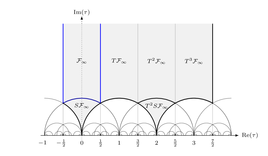
Figure 1: Upper-half plane $\mathbb{H}$ with the area bounded by blue ($\mathcal{F}_{\infty}$) a fundamental domain of $\mathbb{H}/{\rm SL}(2,\mathbb{Z})$, and the shaded area a fundamental domain of $\mathbb{H}/\Gamma^{0}(4)$.

At the cusps $\tau\to 0$ (respectively $\tau\to 2$) a monopole (respectively a dyon) becomes massless, and the effective theory breaks down since additional degrees of freedom need to be taken into account. Another quantity which we will frequently encounter is the derivative $\frac{da}{du}$, which can be expressed as function of $\tau$ as

$$\frac{da}{du}(\tau)=\frac{\vartheta_{2}(\tau)\vartheta_{3}(\tau)}{\Lambda}.$$ (14)

It transforms under the generators of $\Gamma^{0}(4)$ as

$$\begin{split}&\frac{da}{du}(\tau+4)=-\frac{da}{du}(\tau),\\[3.99994pt] &\frac{da}{du}\!\left(\frac{\tau}{\tau+1}\right)=(\tau+1)\,\frac{da}{du}(\tau).\end{split}$$ (15)

2.2 Donaldson-Witten theory

Donaldson-Witten theory is the topologically twisted version of Seiberg-Witten theory with gauge group $\mathrm{SU}(2)$ or $\rm{SO}(3)$ [29]. As mentioned in the introduction, topological twisting preserves a scalar fermionic nilpotent symmetry $\mathcal{Q}$ of the $\mathcal{N}=2$ Yang-Mills theory on an arbitrary four-manifold [1]. For a four-manifold whose holonomy is $\rm{SO}(4)\simeq\rm{SU(2)}_{-}\times\rm{SU}(2)_{+}$ the twist replaces the initially flat ${\rm SU}(2)_{R}$ $R$-symmetry bundle, by the $\rm{SU}(2)_{-}$ subgroup of $\rm{SU}(2)_{-}\times\rm{SU}(2)_{+}$, thereby changing the representations of operators under the rotation group. The original supersymmetry generators transform as the $(\bf{1,2,2})\oplus(2,1,2)$ representation of $\mathrm{SU}(2)_{+}\times\mathrm{SU}(2)_{-}\times\mathrm{SU}(2)_{R}$ group. Their representation under the twisted group $\mathrm{SU}(2)^{\prime}_{+}\times\mathrm{SU}(2)_{-}\times\rm{U}(1)_{R}$ is $({\bf{1,1}})^{+1}\oplus({\bf{2,2}})^{-1}\oplus({\bf{1,3}})^{+1}$. Each term in this direct sum plays an important role in Donaldson-Witten theory. The first term $({\bf{1,1}})^{+1}$ corresponds to the BRST-type operator ${\mathcal{Q}}$ we mentioned above, whose cohomology provides topological invariants of the four-manifold. The second term $({\bf{2,2}})^{-1}$ corresponds to the one-form operator $K$. This operator provides a canonical solution to the descent equations [1]

$$\{\mathcal{Q},\mathcal{O}^{(i+1)}\}=d\mathcal{O}^{(i)},\qquad i=0,\dots,3,$$ (16)

by setting $\mathcal{O}^{(i)}=K^{i}\mathcal{O}^{(0)}$ [8, 9, 10]. Integration of these operators over $i$-cycles gives topological observables since $\{\mathcal{Q},K\}=d$.

Finally, we denote the third representation ${(\bf{1,3})}^{+1}$ by $L$, which will be used to express the ${\mathcal{Q}}$-exact operator (9) in Section 3.3. This operator anti-commutes with the BRST supercharge to give $\{\mathcal{Q},L\}=-(\bar{\sigma}_{mn})^{AB}\bar{Z}_{AB}\,dx^{m}\wedge dx^{n}$, where $m,n$ are ${\rm SO}(4)$ indices while $A,B$ are ${\rm SU}(2)_{R}$ indices. We argue in Appendix C that for a compact Kähler surface $M$, this commutator can be written as

$$\{\mathcal{Q},L\}=\sqrt{2}i\bar{Z}J,$$ (17)

where $\bar{Z}:=\bar{Z}_{12}$ and $J\in\Omega^{1,1}(M)$ the Kähler form associated with the metric $g$ of $M$.

The field content of the low energy topologically twisted theory is a one-form gauge potential $A$, a complex scalar $a$, together with anti-commuting (Grassmann valued) self-dual two-form $\chi$, one-form $\psi$ and zero-form $\eta$. The auxiliary fields of the non-twisted theory combine to a self-dual two-form $D$. The action of the BRST operator $\mathcal{Q}$ on these fields is given by

$$\{\mathcal{Q},A\} =\psi, \{\mathcal{Q},a\} =0, \{\mathcal{Q},\bar{a}\} =\sqrt{2}i\eta,$$

$$\{\mathcal{Q},D\} =(d\psi)_{+}, \{\mathcal{Q},\eta\} =0, \{\mathcal{Q},\psi\} =4\sqrt{2}\,da,$$ (18)

$$\{\mathcal{Q},\chi\} =i(F_{+}-D).$$

Later, it will be useful to express $\mathcal{Q}$ as a derivative in field space,

$$\mathcal{Q}=\psi\,\frac{\partial}{\partial A}+(d\psi)_{+}\frac{\partial}{\partial D}+4\sqrt{2}da\,\frac{\partial}{\partial\psi}+\sqrt{2}i\eta\,\frac{\partial}{\partial\bar{a}}+i(F_{+}-D)\,\frac{\partial}{\partial\chi}.$$ (19)

The low energy Lagrangian of the Donaldson-Witten theory is given by [9]

$$\begin{split}\mathcal{L}&=\frac{i}{16\pi}(\bar{\tau}F_{+}\wedge F_{+}+\tau F_{-}\wedge F_{-})+\frac{y}{8\pi}da\wedge*d\bar{a}-\frac{y}{8\pi}D\wedge*D\\ &\quad-\frac{1}{16\pi}\tau\psi\wedge*d\eta+\frac{1}{16\pi}\bar{\tau}\eta\wedge d*\psi+\frac{1}{8\pi}\tau\psi\wedge d\chi-\frac{1}{8\pi}\bar{\tau}\chi\wedge d\psi\\ &\quad+\frac{\sqrt{2}i}{16\pi}\frac{d\bar{\tau}}{d\bar{a}}\eta\chi\wedge(F_{+}+D)-\frac{\sqrt{2}i}{2^{7}\pi}\frac{d\tau}{da}\psi\wedge\psi\wedge(F_{-}+D)\\ &\quad+\frac{i}{3\cdot 2^{11}}\frac{d^{2}\tau}{da^{2}}\psi\wedge\psi\wedge\psi\wedge\psi-\frac{\sqrt{2}i}{3\cdot 2^{5}\pi}\left\{\mathcal{Q},\chi_{\mu\nu}\chi^{\nu\lambda}\chi_{\lambda}^{\,\,\mu}\right\}\sqrt{g}\,d^{4}x.\end{split}$$ (20)

3 Correlation functions of $\mathcal{Q}$-exact observables

We start in this section an analysis of correlation functions of $\mathcal{Q}$-exact observables to verify the Ward identities (2) and (4). After collecting a few useful facts about four-manifolds with $b_{2}^{+}=1$, we recall the contribution to the path integral of the $u$-plane in Subsection 3.2. In the remainder of the section, we discuss $\mathcal{Q}$-exact observables at an increasing level of generality. We summarize our findings in Subsection 3.6.

3.1 Four-manifolds with $b_{2}^{+}=1$

Let $M$ be a smooth, simply connected, compact four-manifold without boundary. Its basic topological numbers are its Euler character $\chi(M)=2-2b_{1}(M)+b_{2}(M)$ and signature $\sigma(M)=b_{2}^{+}(M)-b_{2}^{-}(M)$, where $b_{1}(M)={\rm dim}(H_{1}(M,\mathbb{R}))$ and $b_{2}^{\pm}(M)={\rm dim}(H_{2}(M,\mathbb{R})^{\pm})$. We will omit the dependence on $M$ unless a confusion may arise. We will restrict in the following to four-manifolds with $b_{2}^{+}=1$, since the $u$-plane integral only contributes for this class of four-manifolds. A four-manifold $M$ with $b_{2}^{+}=1$ admits an almost complex structure, since any simply connected four-manifold with $b_{2}^{+}$ odd does [15]. We denote the canonical class of $M$ by $K_{M}\in H^{2}(M,\mathbb{Z})$, which equals the second Stiefel-Whitney class modulo $H^{2}(M,2\mathbb{Z})$.

The intersection form on the middle cohomology provides a natural bilinear form $B:H^{2}(M,\mathbb{R})\times H^{2}(M,\mathbb{R})\to\mathbb{R}$ that pairs degree two co-cycles,

$$B({\boldsymbol{k}}_{1},{\boldsymbol{k}}_{2}):=\int_{M}{\boldsymbol{k}}_{1}\wedge{\boldsymbol{k}}_{2},$$ (21)

and whose restriction to $H^{2}(M,\mathbb{Z})\times H^{2}(M,\mathbb{Z})$ is an integral bilinear form with signature $(1,b_{2}-1)$. The bilinear form provides the quadratic form $Q({\boldsymbol{k}}):=B({\boldsymbol{k}},{\boldsymbol{k}})\equiv{\boldsymbol{k}}^{2}$, which can be brought to a simple standard form [15, Section 1.1.3]. We denote the period point by $J$, i.e. the harmonic two-form, satisfying

$$*J=J\in H^{2}(M,\mathbb{R}),\qquad J^{2}=1,$$ (22)

with $*$ the Hodge $*$-operation. Using the period point, we can decompose elements ${\boldsymbol{k}}\in H^{2}(M)$ to its self-dual and anti-self-dual components: ${\boldsymbol{k}}_{+}=B({\boldsymbol{k}},J)\,J$ and ${\boldsymbol{k}}_{-}={\boldsymbol{k}}-{\boldsymbol{k}}_{+}$, the anti-self-dual part of ${\boldsymbol{k}}$. For later use, we mention that the canonical class is a characteristic vector of $H^{2}(M,\mathbb{Z})$ and satisfies

$$K_{M}^{2}=\sigma+8.$$ (23)

3.2 Path integral of the Donaldson-Witten theory

We consider Donaldson-Witten theory on a four-manifold $M$ with $b_{2}^{+}=1$ as detailed above. We choose a fixed ’t Hooft flux $[\mathrm{Tr}(F/4\pi)]=2{\boldsymbol{\mu}}\in H^{2}(M,\mathbb{Z})$ for the gauge bundle (we think of $H^{2}(M,\mathbb{Z})$ as a lattice in $H^{2}(M,\mathbb{R})$, thus modding out by torsion). Then we can divide by $2$ and in particular ${\boldsymbol{\mu}}$ can be half-integral.) The Coulomb branch integral $\Phi_{{\boldsymbol{\mu}}}^{J}$ [9] of Donaldson-Witten theory, without any operator insertions, is defined as the usual path integral over the infinite dimensional field space,

$$\Phi_{{\boldsymbol{\mu}}}^{J}=\int[\mathcal{D}a\,\mathcal{D}\bar{a}\,\mathcal{D}A\,\mathcal{D}\eta\,\mathcal{D}\psi\,\mathcal{D}\chi\,\mathcal{D}D]\,e^{-\mathcal{S}}\equiv\langle 1\rangle.$$

We will review in this subsection that the path integral is well-defined and reduces to a modular integral over the domain $\mathbb{H}/\Gamma^{0}(4)$. For the chosen class of four-manifolds, $\Phi_{{\boldsymbol{\mu}}}^{J}$ reduces to a finite dimensional integral over the zero modes [9]. For simplicity, we restrict to simply connected manifolds, $\pi_{1}(M)=0$ and therefore $b_{1}(M)=0$, which do not admit $\psi$ zero modes. The path integral of the effective theory on the Coulomb branch becomes then

$$\Phi_{{\boldsymbol{\mu}}}^{J}=\sum_{{\rm U}(1)\,\,{\rm fluxes}}\int da\wedge d{\bar{a}}\wedge d\eta\wedge d\chi\wedge dD\,\,A(u)^{\chi(M)}\,B(u)^{\sigma(M)}\,e^{-\int_{M}\mathcal{L}_{0}},$$ (24)

where the $a$, $\bar{a}$ and $\eta$ denote now the zero-modes, i.e. they are constant functions on $M$. The Lagrangian $\mathcal{L}_{0}$ is $\mathcal{L}$ (20) restricted to the zero modes including the ones of the gauge field.

The functions $A(u)$ and $B(u)$ are curvature couplings; they are holomorphic functions of $u$, given by [9, 33]

$$\begin{split}A(u)&=\alpha\left(\frac{du}{da}\right)^{\frac{1}{2}},\\[5.0pt] B(u)&=\beta\,(u^{2}-1)^{\frac{1}{8}},\ \end{split}$$ (25)

where we have set $\Lambda=1$, and $\alpha$ and $\beta$ are numerical factors. In more general theories including matter, such as the $N_{f}=4$ theory, they may depend on parameters such as masses and coupling constants.

To integrate over the auxiliary field, let us introduce the Lagrangian $\mathcal{L}_{0,D}$, which consists of the terms in $\mathcal{L}_{0}$ involving $D$,

$$\mathcal{L}_{0,D}=-\frac{y}{8\pi}D\wedge D+\frac{\sqrt{2}i}{16\pi}\frac{d\bar{\tau}}{d\bar{a}}\eta\chi\wedge D.$$ (26)

After a Wick rotation $D\to iD$, the Gaussian integration over its zero mode yields

$$\int dD\,e^{-\int_{M}\mathcal{L}_{0,D}}=2\pi i\sqrt{\frac{2}{y}}.$$ (27)

The only remaining term involving fermion zero-modes in $\mathcal{L}_{0}$ is

$$\mathcal{L}_{0,f}=\frac{\sqrt{2}i}{16\pi}\frac{d\bar{\tau}}{d\bar{a}}\eta\chi\wedge F_{+},$$ (28)

such that integrating over the $\eta$ and $\chi$ zero modes gives

$$\int d\eta\wedge d\chi~{}e^{-\int_{M}\mathcal{L}_{0,f}}=\frac{\sqrt{2}i}{4}\frac{d\bar{\tau}}{d\bar{a}}B({\boldsymbol{k}},J),$$ (29)

where the vector ${\boldsymbol{k}}$ equals the $\rm{U}(1)$ flux $[F]/4\pi\in H^{2}(M,\mathbb{Z})+{\boldsymbol{\mu}}$.

The sum over ${\boldsymbol{k}}$ in (24) takes the form of a Siegel-Narain theta function

$$\Psi^{J}_{\boldsymbol{\mu}}\left[\mathcal{K}_{\rm p}\right](\tau,\bar{\tau})=\sum_{{\boldsymbol{k}}\in\Lambda+{\boldsymbol{\mu}}}\,\mathcal{K}_{\rm p}({\boldsymbol{k}})\,(-1)^{B({\boldsymbol{k}},K_{M})}\,q^{-\frac{{\boldsymbol{k}}_{-}^{2}}{2}}\bar{q}^{\frac{{\boldsymbol{k}}_{+}^{2}}{2}},$$ (30)

where the kernel $\mathcal{K}_{\rm p}$ equals

$$\mathcal{K}_{\rm p}({\boldsymbol{k}})=-\frac{\pi}{\sqrt{y}}\,B({\boldsymbol{k}},{J}),$$ (31)

which follows from multiplying (27) and (29), and dividing by the factor $\frac{d\bar{\tau}}{d\bar{a}}$ since this provides the change of variables from the Coulomb branch parameter $a$ to $\tau\in\mathbb{H}/\Gamma^{0}(4)$. When we consider correlation functions in the next subsection, we will find different expressions for the kernel depending on the inserted fields. Appendix B lists a number of useful properties of $\Psi^{J}_{\boldsymbol{\mu}}[1]$.

We can express the integrand in (24) more compactly, using Matone’s formula [34]

$$\frac{du}{d\tau}=\frac{4\pi}{i}(u^{2}-1)\left(\frac{da}{du}\right)^{2},$$ (32)

and the identities (13) and (14). This gives for $\Phi_{\boldsymbol{\mu}}^{J}$

$$\Phi_{\boldsymbol{\mu}}^{J}=\int_{\mathbb{H}/\Gamma^{0}(4)}d\tau\wedge d\bar{\tau}\,\tilde{\nu}(\tau)\,\Psi_{{\boldsymbol{\mu}}}^{J}[\mathcal{K}_{\rm p}](\tau,\bar{\tau}),$$ (33)

with

$$\tilde{\nu}(\tau):=-8i(u^{2}-1)\frac{da}{du}\vartheta_{4}(\tau)^{\sigma},$$ (34)

and whose modular transformations for the two generators $ST^{-1}S:\tau\mapsto\frac{\tau}{\tau+1}$ and $T^{4}:\tau\mapsto\tau+4$ of $\Gamma^{0}(4)$ are:

$$\begin{split}&\tilde{\nu}\!\left(\frac{\tau}{\tau+1}\right)=(\tau+1)^{2-b_{2}/2}e^{-\frac{\pi i\sigma}{4}}\tilde{\nu}(\tau),\\[5.0pt] &\tilde{\nu}(\tau+4)=-\tilde{\nu}(\tau).\end{split}$$ (35)

The measure $\tilde{\nu}(\tau)$ behaves near the weak coupling cusp $\tau\to i\infty$ as $\sim q^{-\frac{3}{8}}$, and near the monopole cusp, $\tau_{M}=-1/\tau\to i\infty$ as $\sim q_{M}^{1+\frac{\sigma}{8}}$.

An important requirement for (33) is modular invariance of the integrand under $\Gamma^{0}(4)$ transformations. We can easily determine the modular transformations of $\Psi_{{\boldsymbol{\mu}}}^{J}[\mathcal{K}_{\rm p}]$ from those of $\Psi_{{\boldsymbol{\mu}}}^{J}[1]$ (134). The effect of inserting the kernel $\mathcal{K}_{\rm p}$ in $\Psi_{{\boldsymbol{\mu}}}^{J}[1]$ is to increase the weight by $(\frac{1}{2},\frac{3}{2})$. (The factor $1/\sqrt{y}$ contributes $(\frac{1}{2},\frac{1}{2})$ and $B({\boldsymbol{k}},J)$ contributes $(0,1)$ to the total weight.) We then arrive at

$$\begin{split}&\Psi_{{\boldsymbol{\mu}}}^{J}[\mathcal{K}_{\rm p}]\!\left(\frac{\tau}{\tau+1},\frac{\bar{\tau}}{\bar{\tau}+1}\right)=(\tau+1)^{\frac{b_{2}}{2}}(\bar{\tau}+1)^{2}e^{\frac{\pi i}{4}\sigma}\,\Psi_{{\boldsymbol{\mu}}}^{J}[\mathcal{K}_{\rm p}](\tau,\tau),\\[5.0pt] &\Psi_{{\boldsymbol{\mu}}}^{J}[\mathcal{K}_{\rm p}](\tau+4,\bar{\tau}+4)=e^{2\pi iB({\boldsymbol{\mu}},K)}\,\Psi_{{\boldsymbol{\mu}}}^{J}[\mathcal{K}_{\rm p}](\tau,\bar{\tau}),\end{split}$$ (36)

where we used that $K_{M}^{2}=8+\sigma$. We see that the integrand of (33) is invariant under the $\tau\mapsto\frac{\tau}{\tau+1}$ transformation. However, if $B({\boldsymbol{\mu}},K)=0\mod\mathbb{Z}$, the $\tau\mapsto\tau+4$ does multiply the integrand by $-1$, but one can show that $\Psi_{{\boldsymbol{\mu}}}^{J}[\mathcal{K}_{\rm p}]$ vanishes in this case, such that there is no violation of the duality. We conclude therefore that the Coulomb branch integral (33) is well-defined since the measure $d\tau\wedge d\bar{\tau}$ transforms as a mixed modular form of weight $(-2,-2)$ while the product $\tilde{\nu}\,\Psi_{{\boldsymbol{\mu}}}^{J}[\mathcal{K}_{\rm p}]$ is a mixed modular form of weight (2,2) for the congruence subgroup $\Gamma^{0}(4)$.

The evaluation of $\Phi^{J}_{\boldsymbol{\mu}}$ will be discussed in more detail in upcoming work [35]. We will continue in the next subsection by considering correlation functions of BRST exact observables, which need to satisfy the same requirements of modular invariance of the integrand as above. We summarize in Table 1 the weights of the various ingredients that appear in $u$-plane integral for future use.

Ingredient	Mixed weight
$d\tau\wedge d\bar{\tau}$	$(-2,-2)$
$y$	$(-1,-1)$
$\partial_{\bar{\tau}}\,f$	$(k,2)$ if $f$ has weight $(k,0)$
$\tilde{\nu}(\tau)$	$(2-b_{2}/2,0)$
$\Psi_{{\boldsymbol{\mu}}}^{J}[1]$	$\frac{1}{2}((b_{2}-1),1)$

Table 1: Various modular weights for the $u$-plane integral. Transformations are in $\mathrm{SL}(2,\mathbb{Z})$ for the first three rows, while in $\Gamma^{0}(4)$ for the last two rows.

3.3 An anti-holomorphic $\mathcal{Q}$-exact observable

We will analyse in this subsection the $u$-plane integral with the insertion of a specific anti-holomorphic $\mathcal{Q}$-exact surface observable. Our analysis will demonstrate that its vev appears to diverge rather than vanish as suggested by the Ward-Takahashi identity, which will motivate the new regularization in the next section.

The observable of interest is

$$\begin{split}I_{+}({\boldsymbol{x}})&=-\frac{1}{4\pi}\int_{\boldsymbol{x}}\left\{\mathcal{Q},\left\{L,\mathrm{Tr}[\bar{\phi}^{2}]\right\}\right\}\\ &=-\frac{1}{4\pi}\int_{\boldsymbol{x}}\left\{\mathcal{Q},{\rm Tr}[\bar{\phi}\,\chi]\right\},\ \end{split}$$ (37)

where ${\boldsymbol{x}}\in H_{2}(M,\mathbb{Q})$ is a two-cycle, and $L$ is the twisted supersymmetry generator discussed in Section 2.2. The subscript $+$ is to indicate that it involves a self-dual two-form field, and is in a sense a self-dual counterpart of the holomorphic, anti-self dual Donaldson observable $I_{-}({\boldsymbol{x}})$ [24]. Using the action of $L$, we can determine the image of $I_{+}({\boldsymbol{x}})$ in the IR theory, denoted by $\widetilde{I}_{+}({\boldsymbol{x}})$, in terms of the IR fields,

$$\begin{split}\widetilde{I}_{+}({\boldsymbol{x}})&=-\frac{1}{4\pi}\int_{{\boldsymbol{x}}}\left\{\mathcal{Q},\frac{d\bar{u}}{d\bar{a}}\chi\right\}\\ &=-\frac{i}{\sqrt{2}\pi}\int_{{\boldsymbol{x}}}\left(\frac{1}{2}\frac{d^{2}\bar{u}}{d\bar{a}^{2}}\eta\,\chi+\frac{\sqrt{2}}{4}\frac{d\bar{u}}{d\bar{a}}(F_{+}-D)\right).\end{split}$$ (38)

As for the partition function, we first integrate over the $D$ zero mode using (27) and

$$\int dD\,\left[\int_{\boldsymbol{x}}D\right]e^{-\int_{M}\mathcal{L}_{0,D}}=2\pi i\sqrt{\frac{2}{y}}\,\left(\frac{\sqrt{2}i}{4y}\frac{d\bar{\tau}}{d\bar{a}}\,\int_{\boldsymbol{x}}\eta\chi\right).$$ (39)

Next, we integrate over the fermion zero modes; $\int d\eta\wedge d\chi\wedge dD\,\widetilde{I}_{+}({\boldsymbol{x}})\,e^{-\int_{M}\mathcal{L}_{0,f}+\mathcal{L}_{0,D}}$ evaluates to $\frac{d\bar{\tau}}{d\bar{a}}\,\mathcal{K}_{+}({\boldsymbol{k}})$, with $\mathcal{K}_{+}({\boldsymbol{k}})$ given by

$$\mathcal{K}_{+}({\boldsymbol{k}}):=\frac{2\,B({\boldsymbol{x}},J)}{\sqrt{y}}\left(-\frac{1}{2}\frac{d^{2}\bar{u}}{d\bar{a}\,d\bar{\tau}}+\frac{i}{8\,y}\frac{d\bar{u}}{d\bar{a}}+\frac{\pi i}{2}\frac{d\bar{u}}{d\bar{a}}\,{\boldsymbol{k}}_{+}^{2}\right).$$ (40)

Once combined with the sum over the $\rm{U}(1)$ fluxes, Equation (38) can be written in a compact form. One arrives at a total derivative with respect to $\bar{\tau}$,

$$\Psi_{{\boldsymbol{\mu}}}^{J}[\mathcal{K}_{+}](\tau,\bar{\tau})=-\partial_{\bar{\tau}}\left(\frac{B({\boldsymbol{x}},J)}{\sqrt{y}}\,\frac{d\bar{u}}{d\bar{a}}\,\Psi_{{\boldsymbol{\mu}}}^{J}[1](\tau,\bar{\tau})\right).$$ (41)

This expression demonstrates that $\Psi_{{\boldsymbol{\mu}}}^{J}[\mathcal{K}_{+}]$ vanishes for $B({\boldsymbol{\mu}},K_{M})=\frac{1}{2}\mod\mathbb{Z}$, since $\Psi_{{\boldsymbol{\mu}}}^{J}[1]$ vanishes in this case. If non-vanishing $\Psi_{{\boldsymbol{\mu}}}^{J}[\mathcal{K}_{+}]$ has the required modular properties: it transforms with modular weight $(\frac{b_{2}}{2},2)$, and changes by a sign under $\tau\mapsto\tau+4$.

For the one-point function of $\widetilde{I}_{+}({\boldsymbol{x}})$, we arrive at the integral

$$\langle\widetilde{I}_{+}({\boldsymbol{x}})\rangle=-\int_{\mathbb{H}/\Gamma^{0}(4)}d\tau\wedge d\bar{\tau}\,\partial_{\bar{\tau}}\left(\widetilde{\nu}\,\frac{B({\boldsymbol{x}},J)}{\sqrt{y}}\,\frac{d\bar{u}}{d\bar{a}}\,\Psi_{\boldsymbol{\mu}}^{J}[1]\right).$$ (42)

We can easily evaluate this integral using Stokes’ theorem. This reduces to arcs close to the three cusps of $\mathbb{H}/\Gamma^{0}(4)$, $\tau\to i\infty$, $0$ and $2$. But here is where the surprise occurs: since $\frac{d\bar{u}}{d\bar{a}}$ diverges as $\bar{q}^{-\frac{1}{8}}$ for $\tau\to\infty$ and $\tilde{\nu}(\tau)$ as $q^{-\frac{3}{8}}$, we find integrals $L_{m,n,s}$ (7) with both $m$ and $n<0$  for the cusp at $i\infty$! The standard prescription mentioned above Equation (8) therefore does not cure the divergence if $\Psi_{\boldsymbol{\mu}}^{J}\sim q^{\frac{1}{4}}$ for $\tau\to i\infty$. We will explain in Section 5 that the integral can be properly renormalized. This will result in $\langle\widetilde{I}_{+}({\boldsymbol{x}})\rangle=0$, in agreement with the global BRST symmetry.

3.4 General $\mathcal{Q}$-exact observables

Motivated by the example $\widetilde{I}_{+}$, we will make an analysis of general $\mathcal{Q}$-exact observables in this subsection. We assume that these observables satisfy the constraints of single-valuedness on the $u$-plane, and that these would be automatically satisfied if we derive them from $\mathcal{Q}$-exact UV operators. We will find that the $u$-plane integrands for such observables always take the form of a total $\bar{\tau}$-derivative, which facilitates their evaluation in Section 5.

We grade the $\mathcal{Q}$-closed and exact observables by their form degree:

0-form operators

A general 0-form operator $\mathcal{O}_{0}$ can be written as

$$\mathcal{O}_{0}=V_{0}(a,\bar{a})+V_{1}(a,\bar{a})\,\eta,$$ (43)

where we require that $V_{j}$ are real-analytic functions in the real and imaginary part of $a$ on the interior of the $u$-plane, in other words, the $V_{j}$ do not have singularities away from the weak and strong coupling cusps in the $u$-plane. After acting with $\mathcal{Q}$ (2.2) on this expression, we find that the most general $\mathcal{Q}$-exact 0-form operator is

$$\begin{split}G_{0}&=\{\mathcal{Q},\mathcal{O}\}=\sqrt{2}i\,\partial_{\bar{a}}V_{0}(a,\bar{a})\,\eta.\end{split}$$ (44)

The vev $\langle G_{0}\rangle$ vanishes after integration over the fermionic modes, since $G_{0}$ is Grassmann odd and the action only contains Grassmann even terms. We thus find that any 0-form operator satisfies the Ward identity (2). Moreover, any product $\prod_{j}\mathcal{O}_{0,j}$ with $\mathcal{O}_{0,j}$ $\mathcal{Q}$-exact 0-form operators is also of the form (43).

Let us next consider $\mathcal{Q}$-closed 0-form observables. We deduce from (44) that for any $\mathcal{Q}$-closed observable the $\eta^{0}$ term is necessarily holomorphic, thus

$$C_{0}=W_{0}(a)+W_{1}(a,\bar{a})\,\eta,$$ (45)

where $W_{j}$ are again real-analytic functions on the interior of the $u$-plane. For single valuedness of the $u$-plane integrand, $W_{0}$ must be invariant under $\Gamma^{0}(4)$ transformations. For example the famous point operator is $u$. Comparing (44) and (45), we deduce that there exist $\mathcal{Q}$-closed forms, linear in $\eta$, which are not $\mathcal{Q}$-exact. They do however not contribute to correlation functions since they are Grassmann odd. For the same reason, the Ward-Takahashi identity (4) is satisfied for $0$-form observables: for any 0-form observable $\mathcal{O}_{0}$,

$$\langle\{\mathcal{Q},\mathcal{O}_{0}\}\prod_{j}\mathcal{O}_{0,j}\rangle=0,$$ (46)

if all $\mathcal{O}_{0,j}$ are $\mathcal{Q}$-closed 0-form observables.

2-form operators

We continue with $\mathcal{Q}$-exact 2-form operators $G_{2}=\{\mathcal{Q},\mathcal{O}_{2}\}$. We let $\mathcal{O}_{2}$ be the most general 2-form field, expressed as

$$\mathcal{O}=\sum_{X\,\in\{\chi,\,F_{\pm},\,D,\,\psi\wedge\psi\}}V_{X,j}(a,\bar{a})\,\eta^{j}\,X.$$ (47)

where $V_{X,j}(a,\bar{a})$ are again real-analytic functions without singularities away from the strong and weak coupling singularities. Comparing with Equation (38), we find that for $\widetilde{I}_{+}$ the function $V_{\chi,0}(a,\bar{a})$ that

$$V_{\chi,0}(a,\bar{a})=-\frac{1}{4\pi}\frac{d\bar{u}}{d\bar{a}},$$ (48)

and all other $V_{X,j}$ equal to 0. Acting with $\mathcal{Q}$ on $\mathcal{O}$ gives the following expression for $G_{2}$

$$\begin{split}G_{2}&=\sqrt{2}i\,\partial_{\bar{a}}V_{\chi,0}\eta\,\chi+i\,V_{\chi,0}\,(F_{+}-D)\\ &\quad+\sqrt{2}i\,\partial_{\bar{a}}V_{F_{\pm},0}\eta\,F_{\pm}+V_{F_{\pm},0}\,(d\psi)_{\pm}\\ &\quad+\sqrt{2}i\,\partial_{\bar{a}}V_{D,0}\eta\,D+V_{D,0}\,(d\psi)_{+}\\ &\quad+\sqrt{2}i\,\partial_{\bar{a}}V_{\psi\wedge\psi,0}\eta\,\psi\wedge\psi-8\sqrt{2}\,V_{\psi\wedge\psi,0}\,\psi\wedge da\\ &\quad-iV_{\chi,1}\eta\,\,(F_{+}-D)-V_{F_{\pm},1}\eta\,(d\psi)_{\pm}\\ &\quad-V_{D,1}\eta\,(d\psi)_{+}-4\sqrt{2}\,V_{\psi\wedge\psi,1}\eta\,\psi\wedge da,\end{split}$$ (49)

where in the second and fifth line $\pm$ represents a sum over $+$ and $-$.

In correlation functions, we integrate $G_{2}$ over a two-cycle ${\boldsymbol{x}}\in H_{2}(M,\mathbb{Z})$. For simplicity of notation, we set

$$G_{2}({\boldsymbol{x}})\equiv\int_{{\boldsymbol{x}}}G_{2}.$$ (50)

To evaluate $\langle G_{2}({\boldsymbol{x}})\rangle$ for the class of four-manifolds relevant to this paper, we reduce to zero modes and integrate over the $\eta$ and $\chi$ zero-modes. This ensures that all all terms on the right hand side of (49) have a vanishing contribution to $\langle G_{2}({\boldsymbol{x}})\rangle$, except the two terms with $V_{\chi,0}$. We will proceed with only these two terms, which is similar to the analysis in Section 3.3. Integrating over $D$ gives

$$\begin{split}&\int dD\,G_{2}({\boldsymbol{x}})\,e^{-\int_{M}\mathcal{L}_{0,D}}=\\ &\qquad 2\pi i\sqrt{\frac{2}{y}}\left[\int_{\boldsymbol{x}}\left(\sqrt{2}i\,\partial_{\bar{a}}V_{\chi,0}+\frac{\sqrt{2}}{4y}\frac{d\bar{\tau}}{d\bar{a}}V_{\chi,0}\right)\eta\chi+4\pi iV_{\chi,0}\,B({\boldsymbol{k}}_{+},{\boldsymbol{x}})\right].\end{split}$$ (51)

Integrating subsequently over the $\eta$ and $\chi$ zero modes gives the sum over fluxes $\Psi_{\boldsymbol{\mu}}^{J}[\mathcal{K}_{2}]$, with kernel

$$\mathcal{K}_{2}\ =-\frac{4\pi}{\sqrt{y}}\,B({\boldsymbol{x}},J)\left(\partial_{\bar{\tau}}V_{\chi,0}-\frac{i}{4y}V_{\chi,0}-\pi iV_{\chi,0}{\boldsymbol{k}}_{+}^{2}\right),$$ (52)

which can be simplified to

$$\Psi_{{\boldsymbol{\mu}}}^{J}[\mathcal{K}_{2}](\tau,\bar{\tau})=\partial_{\bar{\tau}}\left(\frac{4\pi B({\boldsymbol{x}},J)}{\sqrt{y}}V_{\chi,0}\Psi_{{\boldsymbol{\mu}}}^{J}[1](\tau,\bar{\tau})\right).$$ (53)

We can easily deduce the modular properties of $V_{\chi,0}$ necessary for single-valuedness of the integrand: $V_{\chi,0}$ must have weight $(0,-1)$, and transform with the same multiplier system as $d\bar{u}/d\bar{a}$.

Our next aim is to consider correlation functions of a $\mathcal{Q}$-exact operator with a $\mathcal{Q}$-closed operator. To this end, let us analyze the form of the most general $\mathcal{Q}$-closed two-form operator $C_{2}=\sum_{X}W_{X,j}X\,\eta^{j}$. Since we integrate over a closed two-cycle, $\int_{\boldsymbol{x}}\mathcal{O}$, the right hand side of (49) can vanish up to a total derivative. The relations this imposes on the functions $W_{*,j}$ are easily read off from (49). We obtain

$$W_{\psi\wedge\psi,0}=\frac{1}{8\sqrt{2}}\partial_{a}W_{F_{-},0},\qquad W_{\chi,1}=\sqrt{2}\partial_{\bar{a}}W_{F_{+},0},$$

$$W_{F_{-},0}=W_{F_{+},0}+W_{D,0}=\text{holomorphic},$$ (54)

$$W_{D,1}+W_{F_{+},1}=W_{F_{-},1}=W_{\psi\wedge\psi,1}=W_{\chi,0}=0.$$

Then we see that $C_{2}$ can be expressed as

$$\begin{split}C_{2}&=W_{F_{-},0}\,(F_{-}+D)+\frac{1}{8\sqrt{2}}\partial_{a}W_{F_{-},0}\,\psi\wedge\psi\\ &\quad+\sqrt{2}\partial_{\bar{a}}W_{F_{+},0}\eta\chi+W_{F_{+},0}\,(F_{+}-D)\\ &\quad+W_{F_{+},1}(a,\bar{a})\,\eta\,(F_{+}-D),\end{split}$$ (55)

and

$$\{\mathcal{Q},C_{2}\}=d\left(W_{F_{-},0}(a)\,\psi\right).$$ (56)

The first two terms in (55) are holomorphic and do match the terms in the standard Donaldson surface observable as derived using the descent formalism. Comparing with Equation (2.17) in [9], we find that for the surface observable

$$W_{F_{-},0}(a)=-\frac{i}{4\pi}\frac{du}{da}.$$ (57)

The last three terms on the rhs of (55) are $\mathcal{Q}$-exact, and the first two are of form which do not automatically vanish.

We consider next the correlation function for the product of a $\mathcal{Q}$-exact and a $\mathcal{Q}$-closed operator, $G_{2}({\boldsymbol{x}})\,C_{2}({\boldsymbol{x}}^{\prime})$. As before, the path integral restricts to zero modes and Grassmann even terms. Integration over the zero modes of $D$, $\eta$ and $\chi$ gives

$$\begin{split}&\int d\eta\wedge d\chi\wedge dD\,G_{2}({\boldsymbol{x}})\,C_{2}({\boldsymbol{x}}^{\prime})\,e^{-\int_{M}\mathcal{L}_{0,D}+\mathcal{L}_{0,f}}=\\ &\quad 16\pi^{2}\,\frac{d\bar{\tau}}{d\bar{a}}\,B({\boldsymbol{x}},J)\,B({\boldsymbol{x}}^{\prime},J)\,B({\boldsymbol{k}},J)\left[\left(\partial_{\bar{\tau}}\frac{V_{\chi,0}W_{F_{+},0}}{\sqrt{y}}\right)-\frac{V_{\chi,0}W_{F_{+},0}}{\sqrt{y}}\,\pi i{\boldsymbol{k}}_{+}^{2}\right]\\ &\quad+16\pi^{2}\,\frac{d\bar{\tau}}{d\bar{a}}\,W_{F_{-}}\,B({\boldsymbol{x}},J)\,B({\boldsymbol{x}}^{\prime},{\boldsymbol{k}}_{-})\,\left[\left(\partial_{\bar{\tau}}\frac{V_{\chi,0}}{\sqrt{y}}\right)-\frac{V_{\chi,0}}{\sqrt{y}}\,\pi i{\boldsymbol{k}}_{+}^{2}\right],\end{split}$$ (58)

where the first line is due to the product of the non-holomorphic $\mathcal{Q}$-exact part of $C_{2}$ with $G_{2}$, and the second line is the contribution of the product from the holomorpic part of $C_{2}$ with $G_{2}$. Note that the term in brackets on the second line is very similar to (52), since the holomorphic part commutes with $\partial_{\bar{\tau}}$. Using (58), we may write the $u$-plane integrand for $\langle G_{2}({\boldsymbol{x}})\,C_{2}({\boldsymbol{x}}^{\prime})\rangle$ as

$$\begin{split}&B({\boldsymbol{x}},J)\,B({\boldsymbol{x}}^{\prime},J)\,\partial_{\bar{\tau}}\!\left(\widetilde{\nu}\,V_{\chi,0}\,W_{F_{+},0}\,\Psi_{\boldsymbol{\mu}}^{J}[\mathcal{K}_{2}^{(2)}/i]\right)\\ &+B({\boldsymbol{x}},J)\,\partial_{\bar{\tau}}\!\left(\widetilde{\nu}\,W_{F_{-},0}\,V_{\chi,0}\,\Psi_{\boldsymbol{\mu}}^{J}[\mathcal{K}_{-}]\right),\end{split}$$ (59)

where the kernels read

$$\begin{split}\mathcal{K}_{2}^{(2)}&=\frac{16\pi^{2}i}{\sqrt{y}}\,B({\boldsymbol{k}},J),\qquad\mathcal{K}_{-}=\frac{16\pi^{2}}{\sqrt{y}}B({\boldsymbol{x}}^{\prime},{\boldsymbol{k}}_{-}).\end{split}$$ (60)

We have thus demonstrated that the $u$-plane integral takes for this correlator also the form of a total derivative. We will not develop further products of $\mathcal{Q}$-closed 2-form operators multiplied by a $\mathcal{Q}$-exact operator, which will require contact terms [9, 10]. Such cases are included implicitly in the discussion in on the “General $\mathcal{Q}$-exact operator”.

We can give a closed expression for an arbitrary product of $\mathcal{Q}$-exact two-form operators,

$$\left\langle\prod_{j=1}^{\ell}G_{2}^{(j)}({\boldsymbol{x}}_{j})\right\rangle,$$ (61)

with

$$G_{2}^{(j)}=\sqrt{2}i\,\partial_{\bar{a}}V^{(j)}\,\eta\,\chi+iV^{(j)}\,(F_{+}-D),\qquad j=1,\dots,\ell.$$ (62)

We will prove below that the sum over fluxes can written as the following total derivative

$$\partial_{\bar{\tau}}\left(\left(\prod_{j=1}^{\ell}B({\boldsymbol{x}}_{j},J)\,V^{(j)}\right)\,\Psi_{\boldsymbol{\mu}}^{J}[\mathcal{K}_{2}^{(\ell)}]\right),$$ (63)

where the kernel $\mathcal{K}^{(\ell)}_{2}$ is given by Equation (80) in terms of the Hermite polynomial $H_{\ell-1}$. The results of Vignéras [36] imply that the integrand single valued if the $V^{(j)}$ transform as $d\bar{u}/d\bar{a}$.

We have thus demonstrated that any product of $\mathcal{Q}$-exact two-form observables can be expressed as a total $\bar{\tau}$-derivative. The form of the kernel ensures moreover that the integrand is well-defined, as long as the functions $V^{(\ell)}$ transform with the same weight and multiplier system as $\frac{d\bar{u}}{d\bar{a}}$ under $\Gamma^{0}(4)$ transformations.

4-form operators

We can similarly treat the most general $\mathcal{Q}$-exact 4-form operator. If we leave aside terms which have an odd number of fermionic fields and terms involving derivatives, the most general operator has the form

$$\begin{split}G_{4}&=\left\{\mathcal{Q},V_{\chi,F_{+}}\chi\wedge F_{+}+V_{\chi,D}\chi\wedge D\right\}\\ &=\sqrt{2}i\partial_{\bar{a}}V_{\chi,F_{+}}\,\eta\chi\wedge F_{+}+i\,V_{\chi,F_{+}}\,(F_{+}-D)\wedge F_{+}\\ &\quad+iV_{\chi,D}(F_{+}-D)\wedge D.\end{split}$$ (64)

We aim to evaluate $\langle\int_{M}G_{4}\rangle$. Using (27), (39) and

$$\begin{split}&\int dD\,\left[\int_{M}D\wedge D\right]\,e^{-\int_{M}\mathcal{L}_{0,D}}=-\frac{8\pi^{2}i}{y}\sqrt{\frac{2}{y}},\end{split}$$ (65)

we find

$$\begin{split}&\int dD\,\int_{M}G_{4}\,e^{-\int_{M}\mathcal{L}_{0,D}}=2\pi i\sqrt{\frac{2}{y}}\left[\sqrt{2}i\partial_{\bar{a}}V_{\chi,F_{+}}\,\int_{M}\eta\chi\wedge F_{+}\right.\\ &\left.\qquad+i\,V_{\chi,F_{+}}\,\int_{M}(F_{+}-i\frac{\sqrt{2}}{4y}\frac{d\bar{\tau}}{d\bar{a}}\,\eta\chi)\wedge F_{+}+iV_{\chi,D}\int_{M}(F_{+}\wedge i\frac{\sqrt{2}}{4y}\frac{d\bar{\tau}}{d\bar{a}}\eta\chi)+\frac{4\pi i}{y}V_{\chi,D}\right]\end{split}$$ (66)

Integrating over the fermionic zero-modes gives the kernel $\mathcal{K}_{4}$ for $\Psi_{\boldsymbol{\mu}}^{J}$,

$$\mathcal{K}_{4}({\boldsymbol{k}})=\frac{8\sqrt{2}\pi^{2}B({\boldsymbol{k}},J)}{\sqrt{y}}\left(\partial_{\bar{\tau}}V_{\chi,F_{+}}-\frac{i}{4y}V_{\chi,F_{+}}-\pi iV_{\chi,F_{+}}{\boldsymbol{k}}_{+}^{2}\right).$$ (67)

Also $\Psi_{\boldsymbol{\mu}}^{J}[\mathcal{K}_{4}]$ can be expressed as an anti-holomorphic derivative in accordance to the previous subsection

$$\Psi_{\boldsymbol{\mu}}^{J}[\mathcal{K}_{4}]=4\sqrt{2}i\partial_{\bar{\tau}}\left(V_{\chi,F_{+}}\Psi_{{\boldsymbol{\mu}}}^{J}[\mathcal{K}_{\rm{p}}]\right).$$ (68)

with $\mathcal{K}_{\rm p}$ as in (31).

General $\mathcal{Q}$-exact operator

We have seen now a number of classes of $\mathcal{Q}$-exact operators, whose $u$-plane integrand can be expressed as a total derivative with respect to $\bar{\tau}$. We will demonstrate that this is not a coincidence but a generic phenomenon. To this end, we reduce to the zero-mode sector from the beginning and include the $\mathcal{Q}$-exact part of the Lagrangian in the observable. Recall that the zero-mode Lagrangian can be expressed as

$$\mathcal{L}_{0}=\frac{i}{8\pi}\tau F\wedge F+\left\{\mathcal{Q},W\right\},$$ (69)

with $W=-\frac{i}{8\pi}\,y\,\chi\,(F_{+}+D)$. We can rewrite

$$\left\{\mathcal{Q},\mathcal{O}\right\}\,e^{-\mathcal{L}_{0}}=\left\{\mathcal{Q},\widetilde{\mathcal{O}}\right\}\,q^{-{\boldsymbol{k}}^{2}/2},$$ (70)

with $\widetilde{\mathcal{O}}=\mathcal{O}\,e^{-\int_{M}\left\{\mathcal{Q},W\right\}}$. This will simplify the integrations over the fermion and auxiliary zero modes.

To this end, let us expand $\widetilde{\mathcal{O}}$ in terms of $\eta$ and $\chi$, and integrate $\chi$ over a cycle ${\boldsymbol{x}}\in H_{2}(M,\mathbb{Q})$, such that the operator $\widetilde{\mathcal{O}}\in H_{0}(M)$. The expansion then reads

$$\widetilde{\mathcal{O}}({\boldsymbol{x}})=\sum_{m=0,1}\widetilde{\mathcal{O}}_{m,0}\,\eta^{m}+\sum_{m=0,1}\widetilde{\mathcal{O}}_{m,1}\,\eta^{m}\,\int_{\boldsymbol{x}}\chi,$$ (71)

where $\widetilde{\mathcal{O}}_{m,n}$ are functions of $a$, $\bar{a}$, $\int F$ and $\int D$. With the $\mathcal{Q}$-commutaters (2.2) restricted to zero modes, we have

$$\left\{\mathcal{Q},\widetilde{\mathcal{O}}({\boldsymbol{x}})\right\}=\sqrt{2}i\partial_{\bar{a}}\widetilde{\mathcal{O}}_{0,0}\,\eta+\sqrt{2}i\partial_{\bar{a}}\widetilde{\mathcal{O}}_{0,1}\,\eta\,\int_{\boldsymbol{x}}\chi-i\int_{\boldsymbol{x}}(F_{+}-D)\sum_{m=0,1}\widetilde{\mathcal{O}}_{m,1}\,\eta^{m}.$$ (72)

Only the term with $\widetilde{\mathcal{O}}_{0,1}$ survives the integration over fermion zero modes,

$$\int d\eta\,d\chi\,\left\{\mathcal{Q},\widetilde{\mathcal{O}}({\boldsymbol{x}})\right\}=-\sqrt{2}i\,B({\boldsymbol{x}},J)\,\partial_{\bar{a}}\widetilde{\mathcal{O}}_{0,1},$$ (73)

where

$$\widetilde{\mathcal{O}}_{0,1}=\mathcal{O}_{0,1}\,q^{-{\boldsymbol{k}}_{-}^{2}/2}\bar{q}^{{\boldsymbol{k}}_{+}^{2}/2}\,\exp\!\left(\frac{y}{8\pi}\int_{M}D^{2}\right).$$ (74)

We thus find that the $u$-plane integrand can be expressed as a total $\bar{\tau}$-derivative for any $\mathcal{Q}$-exact observable. Moreover, the only term of $\widetilde{\mathcal{O}}$ which contributes to the integrand is linear in $\chi$ and independent of $\eta$.

Let us consider a product $\prod_{j=1}^{\ell}G_{2}({\boldsymbol{x}}_{j})$ of $\mathcal{Q}$-exact operators. We can express this as $\{\mathcal{Q},\mathcal{O}^{(\ell)}\}$, with

$$\mathcal{O}^{(\ell)}=V^{(1)}\,\int_{{\boldsymbol{x}}_{1}}\chi\,\times\prod_{j=2}^{\ell}G_{2}^{(j)}({\boldsymbol{x}}_{j}),$$ (75)

with $G_{2}^{(j)}$ as in (62). The coefficient of $\eta^{0}\,\int_{{\boldsymbol{x}}_{1}}\chi$, $\mathcal{O}^{(\ell)}_{0,1}$, of this operator is given by

$$\mathcal{O}_{0,1}^{(\ell)}=i^{\ell-1}B(F_{+}-D,J)^{\ell-1}\,V^{(1)}\,\prod_{j=2}^{\ell}V^{(j)}\,B({\boldsymbol{x}}_{j},J).$$ (76)

Integrating out $D$ leads to expressions in terms of the Hermite polynomials as suggested below Equation (63). To this end, recall the following integral formula for the Hermite polynomials,

$$H_{\ell}(s)=\frac{2^{\ell}}{\sqrt{\pi}}\int^{\infty}_{-\infty}dt\,(s-it)^{\ell}\,e^{-t^{2}}.$$ (77)

The first few $H_{\ell}$ read

$$\begin{split}&H_{0}(s)=1,\\ &H_{1}(s)=2s,\\ &H_{2}(s)=4s^{2}-2.\end{split}$$ (78)

Using the identity (77), we find

$$\begin{split}&\int dD\,\mathcal{O}^{(\ell)}_{0,1}\,\exp\!\left(\frac{y}{8\pi}\int_{M}D^{2}\right)=\\ &\qquad 2\sqrt{\pi}\left(i\sqrt{\frac{2\pi}{y}}\right)^{\ell}\,H_{\ell-1}(\sqrt{2\pi y}\,B({\boldsymbol{k}},J))\,\prod_{j=1}^{\ell}V^{(j)}\,B({\boldsymbol{x}}_{j},J).\end{split}$$ (79)

We now arrive at Equation (63) for the sum over fluxes, with kernel $\mathcal{K}^{(\ell)}_{2}$

$$\mathcal{K}^{(\ell)}_{2}=-2i\sqrt{2\pi}\left(i\sqrt{\frac{2\pi}{y}}\right)^{\ell}\,H_{\ell-1}(\sqrt{2\pi y}\,B({\boldsymbol{k}},J)).$$ (80)

3.5 A holomorphic self-dual operator

We have seen in the previous subsections examples of a holomorphic operator combined with anti-selfdual field strength, and an anti-holomorphic operator combined with a self-dual field strength. The low energy expressions illustrate that they neatly satisfy the constraints of the duality group. In this section, we consider a $\mathcal{Q}$-exact operator which is holomorphic in $a$ and involves a self-dual field strength. We denote the UV operator by $I_{\diamond}$, which reads explicitly

$$I_{\diamond}({\boldsymbol{x}})=\int_{{\boldsymbol{x}}}\{{\mathcal{Q}},\text{Tr}[\phi\,\chi]\}.$$ (81)

Since the integrand is not a descendant of $K$ or $L$, the IR operator $\widetilde{I}_{\diamond}({\boldsymbol{x}})$ does not follow straightforwardly from the UV expression. The discussion in this subsection is therefore of a more speculative nature.

We take the following Ansatz for the IR observable

$$I_{\diamond}({\boldsymbol{x}})\xrightarrow[\text{}]{\text{RG flow}}\widetilde{I}_{\diamond}({\boldsymbol{x}})=\int_{\boldsymbol{x}}\left(\frac{du}{da}\left(\,F_{+}-D\right)+g(\tau)\,\frac{du}{da}\,\left(\,F_{+}+D\right)\right),$$ (82)

where $g(\tau)$ is an unknown function, which we aim to fix below. From the UV definition, one would expect that $g$ vanishes, but we will see below that the integrand is not modular invariant in that case. We will require that $g$ is a non-perturbative correction, and vanishes exponentially fast in the weak-coupling limit $\tau\to i\infty$. We will then demonstrate that $g$ is uniquely determined by modularity.

Integration over the fermion zero modes after insertion of $\widetilde{I}_{\diamond}({\boldsymbol{x}})$, leads to the kernel

$$\begin{split}\mathcal{K}_{\diamond}({\boldsymbol{k}})=&\frac{iB({\boldsymbol{x}},J)}{2\sqrt{2y}}\,\frac{du}{da}\,\left\{\left(4\pi\,{\boldsymbol{k}}_{+}^{2}+\frac{1}{y}\right)-g(\tau)\left(4\pi\,{\boldsymbol{k}}_{+}^{2}-\frac{1}{y}\right)\right\}.\end{split}$$ (83)

To satisfy the requirements that the integrand is $\Gamma^{0}(4)$ invariant and $g$ is non-perturbative, we set

$$g(\tau)=\frac{\pi}{6}\left(2E_{2}(\tau)-\vartheta_{3}(\tau)^{4}-\vartheta_{4}(\tau)^{4}\right)=-16\pi\,q+O(q^{2}),$$ (84)

where $E_{2}$ is the Eisenstein series, and the $\vartheta_{j}$ are Jacobi theta series (128). We set furthermore

$$\widehat{g}(\tau)=\frac{\pi}{6}\left(2\widehat{E}_{2}(\tau)-\vartheta_{3}(\tau)^{4}-\vartheta_{4}(\tau)^{4}\right),$$ (85)

with $\widehat{E}_{2}(\tau)$ the non-holomorphic Eisenstein series $\widehat{E}_{2}(\tau)=E_{2}(\tau)-\frac{3}{\pi y}$. We see that $\widehat{g}$ transforms as a weight two modular form of $\Gamma^{0}(4)$, and that for $\tau\to i\infty$, the function $\widehat{g}(\tau)$ behaves as $-\frac{1}{y}+O(q)$. We can now express $\Psi_{\boldsymbol{\mu}}^{J}$ as a total derivative to $\bar{\tau}$

$$\Psi_{\boldsymbol{\mu}}^{J}[\mathcal{K}_{\diamond}](\tau,\bar{\tau})=\frac{i}{2}B({\boldsymbol{x}},J)\frac{du}{da}\,\frac{d}{d\bar{\tau}}\left(\sqrt{y}\,\widehat{g}(\tau)\,\Psi_{\boldsymbol{\mu}}^{J}[1](\tau,\bar{\tau})\right),$$ (86)

where as before we have not included the term $\frac{d\bar{\tau}}{d\bar{a}}$, which is the Jacobian for the change of variable to $\bar{\tau}$. One may verify that $\Psi_{\boldsymbol{\mu}}^{J}[\mathcal{K}_{\diamond}]$ has the same transformation properties as $\Psi_{\boldsymbol{\mu}}^{J}[\mathcal{K}_{+}]$.

3.6 Summary

Let us give a summary of the results of this section. We have found that vacuum expectation values of $\mathcal{Q}$-exact operators can be expressed as integrals whose integrands can be written as a total $\bar{\tau}$-derivative after integration over the auxiliary field $D$ and the fermionic zero modes. The vev of a $\mathcal{Q}$-exact operator takes therefore the form

$$\langle\left\{\mathcal{Q},\mathcal{O}\right\}\rangle=\int_{\mathbb{H}/\Gamma^{0}(4)}d\tau\wedge d\bar{\tau}\,\partial_{\bar{\tau}}\left(\widetilde{\nu}\,\,W_{\mathcal{O}}\,\Psi_{\boldsymbol{\mu}}^{J}[\mathcal{K}_{\mathcal{O}}]\right),$$ (87)

for some non-holomorphic function $W_{\mathcal{O}}$ and kernel $\mathcal{K}_{\mathcal{O}}$, which both depend on $\mathcal{O}$. Given the total derivative, we can easily evaluate the integral using Stokes’ theorem, which reduces the integral to three arcs around the cusps of $\mathbb{H}/\Gamma^{0}(4)$.

For a more standard treatment, we map the integral over $\mathbb{H}/\Gamma^{0}(4)$ to an integral over $\mathcal{F}_{\infty}$, by mapping the six $\mathrm{SL}(2,\mathbb{Z})/\Gamma^{0}(4)$ images of $\mathcal{F}_{\infty}$ in $\mathbb{H}/\Gamma^{0}(4)$ back to $\mathcal{F}_{\infty}$. Equation (87) can then be expressed as

$$\langle\left\{\mathcal{Q},\mathcal{O}\right\}\rangle=\int_{\mathcal{F}_{\infty}}d\tau\wedge d\bar{\tau}\,\partial_{\bar{\tau}}F_{\mathcal{O}},$$ (88)

where $F_{\mathcal{O}}$ is the sum of the six transformations of $\widetilde{\nu}\,\,W_{\mathcal{O}}\,\Psi_{\boldsymbol{\mu}}^{J}[\mathcal{K}_{\mathcal{O}}]$ by the elements of $\mathrm{SL}(2,\mathbb{Z})/\Gamma^{0}(4)$. It has a $q$-expansion of the form

$$F_{\mathcal{O}}=y^{-s}\sum_{m,n}c(m,n)\,q^{m}\bar{q}^{n},$$ (89)

or a finite sum of such terms with different $s$. For the $\mathcal{Q}$-exact operator $\widetilde{I}_{+}({\boldsymbol{x}})$, we have seen that $m$ and $n$ can be both negative leading to a divergence for $\tau\to i\infty$. Moreover, it is possible that $m=n<0$, for which the standard renormalization does not apply. We introduce a new renormalization prescription in the next section which also allows us to work with operators leading to terms with $m=n<0$.

4 Renormalization of modular integrals

The previous section discussed the importance of integrals of the form

$$\mathcal{I}_{f}=\int_{\mathcal{F}}d\tau\wedge d\bar{\tau}\,y^{-s}\,f(\tau,\bar{\tau}),$$ (90)

for supersymmetric field theories, where $f$ is a non-holomorphic modular form of weight $(2-s,2-s)$, and $\mathcal{F}$ a fundamental domain for the modular group, $\mathcal{F}=\mathbb{H}/{\rm SL}(2,\mathbb{Z})$. We will discuss in this section the evaluation, regularization and renormalization of integrals of this form, which has been developed in the mathematical literature in the context of inner products for weakly holomorphic modular forms [26].

4.1 Renormalization of integrals over $\mathcal{F}_{\infty}$

We start by considering the integral over a single term $q^{m}\,\bar{q}^{n}$ in the Fourier expansion of $f$. To this end, consider the set $\mathcal{T}$ of triples $(m,n,s)$, defined by

$$\mathcal{T}=\left\{m,n\in\mathbb{R},s\in\mathbb{Z}/2\,|\,m-n\in\mathbb{Z}\right\}.$$ (91)

For $(m,n,s)\in\mathcal{T}$, we consider the integral

$$L_{m,n,s}=\int_{\mathcal{F}_{\infty}}d\tau\wedge d\bar{\tau}\,y^{-s}\,q^{m}\bar{q}^{n},$$ (92)

where $\mathcal{F}_{\infty}$ is the common keyhole fundamental domain $\mathcal{F}=\mathbb{H}/\mathrm{SL}(2,\mathbb{Z})$ pictured in Figure 1. Since $\mathcal{F}_{\infty}$ is non-compact and the integrand may diverge for $y\to\infty$, this is an improper integral. It should be understood as the limiting value of integrals over compact domains, which approach $\mathcal{F}_{\infty}$. To this end, we introduce the compact domain $\mathcal{F}_{Y}$ by restricting $\mathrm{Im}(\tau)\leq Y$ for some $Y\geq 1$. The boundaries of $\mathcal{F}_{Y}$ are given by the following arcs

$$\begin{split}&1:\quad\tau=\tfrac{1}{2}+iy,\qquad\,\,\,\,y\in[\tfrac{1}{2}\sqrt{3},Y],\\ &2:\quad\tau=x+iY,\qquad\,\,\,\,x\in[-\tfrac{1}{2},\tfrac{1}{2}],\\ &3:\quad\tau=-\tfrac{1}{2}+iy,\qquad y\in[\tfrac{1}{2}\sqrt{3},Y],\\ &4:\quad\tau=i\,e^{i\varphi},\qquad\,\,\,\,\,\,\,\,\,\,\,\,\varphi\in[-\tfrac{\pi}{6},\tfrac{\pi}{6}].\\ \end{split}$$ (93)

In the limit, $\lim_{Y\to\infty}\mathcal{F}_{Y}$ we recover $\mathcal{F}_{\infty}$. We then regularize $L_{m,n,s}$ as

$$L_{m,n,s}(Y)=\int_{\mathcal{F}_{Y}}d\tau\wedge d\bar{\tau}\,y^{-s}\,q^{m}\bar{q}^{n},$$ (94)

for $(m,n,s)\in\mathcal{T}$, and define

$$L_{m,n,s}=\lim_{Y\to\infty}L_{m,n,s}(Y),$$ (95)

provided the limit exists. To study the dependence on $Y$, we split the compact domain $\mathcal{F}_{Y}$ into $\mathcal{F}_{1}$ plus a rectangle $[-\frac{1}{2},\frac{1}{2}]\times[1,Y]$ as shown below in Figure 2.

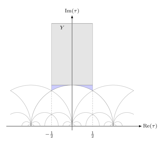
Figure 2: Splitting of $\mathcal{F}_{Y}$ into $\mathcal{F}_{1}$ (the blue region) and the rectangle $\mathcal{R}_{Y}$ (gray region).

The split of $\mathcal{F}_{Y}$, gives for $L_{m,n,s}(Y)$

$$\begin{split}L_{m,n,s}(Y)=&\int_{\mathcal{F}_{1}}d\tau\wedge d\bar{\tau}\,y^{-s}\,q^{m}\bar{q}^{n}-2i\int_{-\frac{1}{2}}^{\frac{1}{2}}\int_{1}^{Y}dx\wedge dy\,\,y^{-s}\,q^{m}\bar{q}^{n}.\end{split}$$ (96)

The first term on the right hand side is finite and independent of $Y$. In the second term, we integrate over $x$, which gives zero unless $m=n$,

$$-2i\,\delta_{m,n}\int_{1}^{Y}dy\,\,y^{-s}\,e^{-4\pi my}.$$ (97)

We thus find that $\lim_{Y\to\infty}L_{m,n,s}(Y)$ converges, except if $m=n<0$, or if $m=n=0$ with $s\leq 1$. Let us denote this set by $\mathcal{D}$,

$$\mathcal{D}=\left\{(m,n,s)\in\mathcal{T}\,|\,m=n<0\right\}\cup\left\{(0,0,s)\in\mathcal{T}\,|\,s\leq 1\right\}.$$ (98)

The correlation functions discussed in Section 3 give rise to $(m,n,s)\in\mathcal{D}$, suggesting that $\mathcal{Q}$-exact observables appear to diverge rather than vanish. To resolve the tension of this divergence with the structure of topologically twisted theories, we aim to regularize and renormalize such integrals. The cases with $m=n=0$ are renormalized in the standard way [19, 20, 22]: as the constant term of the integral for sufficiently large $s$, which gives 0 for (97) if $s=1$ and otherwise $2i/(s-1)$. To treat the cases with $m=n<0$, we put forward in this section a regularized and renormalized version $L^{\rm r}_{m,n,s}$, of $L_{m,n,s}$ for all $(m,n,s)\in\mathcal{T}$.

Before introducing $L^{\rm r}_{m,n,s}$, let us note that the limit of the sum

$$\lim_{Y\to\infty}\left[L_{m,n,s}(Y)+2i\,\delta_{m,n}\int_{1}^{Y}dy\,\,y^{-s}\,e^{-4\pi my}\right]=L_{m,n,s}(1),$$ (99)

is finite. In the definition for $L^{\rm r}_{m,n,s}$, we will subtract from the two terms in the brackets, an appropriately regularized counter part of the second term. To this end, let us introduce the generalized exponential integral $E_{\ell}(z)$. For $\mathrm{Re}(z)>0$, $E_{\ell}(z)$ is defined by

$$E_{\ell}(z)=\int_{1}^{\infty}e^{-z\,t}t^{-\ell}dt.$$ (100)

Integral shifts of the parameter $\ell$ are related by partial integration

$$e^{-z}=z\,E_{\ell}(z)+\ell\,E_{\ell+1}(z).$$ (101)

We can also express $E_{\ell}(z)$ in terms of the incomplete Gamma function $\Gamma(k,z)$,

$$\Gamma(k,z)=\int_{z}^{\infty}e^{-t}\,t^{k-1}dt=z^{k}E_{1-k}(z).$$ (102)

With the analytic continuation of $\Gamma(k,z)$, we can extend the domain of $E_{\ell}(z)$ to the full complex plane. We define

$$E_{\ell}(z)=\begin{cases}\quad z^{\ell-1}{\displaystyle\int_{z}}^{\,\infty}e^{-t}\,t^{-\ell}~{}dt,&\text{for }z\in\mathbb{C}^{*},\\ &\\ \quad\quad\quad\quad\displaystyle{\frac{1}{\ell-1}},&\text{for }z=0,\,\,\ell\neq 1,\\ &\\ \quad\quad\quad\quad\quad 0,&\text{for }z=0,\,\,\ell=1,\end{cases}$$ (103)

where for non-integral $\ell$, we fix the branch of $t^{-\ell}$ by specifying that the argument of any complex number $\rho\in\mathbb{C}^{*}$ is in the domain $(-\pi,\pi]$. For $s\in\mathbb{R}^{+}$, we have $\mathrm{Im}(E_{\ell}(-s))=\pm\frac{\pi\,s^{\ell-1}}{\Gamma(\ell)}$, where the sign is $+$ if the contour $[-s,\infty)$ is deformed to the lower half plane of the complex half-plane to avoid the singularity at $t=0$, and the sign is $-$ if the contour is deformed to the upper half-plane.

In terms of this function $E_{\ell}(z)$, we finally define $L^{\rm r}_{m,n,s}$ for all $(m,n,s)\in\mathcal{T}$:

$$\begin{split}L^{\rm r}_{m,n,s}&=\int_{\mathcal{F}_{1}}d\tau\wedge d\bar{\tau}\,y^{-s}\,q^{m}\bar{q}^{n}-2i\,\delta_{m,n}\,E_{s}(4\pi m),\end{split}$$ (104)

which regularizes and renormalizes the ill-defined $L_{m,n,s}$.

4.2 Modular invariant integrands

We provide in this subsection the prescription to renormalize $\mathcal{I}_{f}$. Let us start with the integral of a modular form over the fundamental domain,

$$\mathcal{I}_{f}=\int_{\mathcal{F}_{\infty}}d\tau\wedge d\bar{\tau}\,y^{-s}\,f(\tau,\bar{\tau}),$$ (105)

where $f(\tau,\bar{\tau})$ is a non-holomorphic modular form for ${\rm SL}(2,\mathbb{Z})$ of weight $(2-s,2-s)$, with Fourier expansion

$$f(\tau,\bar{\tau})=\sum_{m,n\gg-\infty}\,c(m,n)\,q^{m}\bar{q}^{n},$$ (106)

where the $c(m,n)$ are only non-zero if $m-n\in\mathbb{Z}$ by the requirement that $f$ is a modular form. We assume that $f$ is in fact a function on $\mathbb{H}\times\mathbb{\bar{H}}$, which satisfies

$$f\!\left(\frac{a\tau+b}{c\tau+d},\frac{a\sigma+b}{c\sigma+d}\right)=(c\tau+d)^{2-s}(c\sigma+d)^{2-s}f(\tau,\sigma),$$ (107)

where for $s\in\mathbb{Z}+\tfrac{1}{2}$, we specify the branch of the square root by requiring that the argument of $c\tau+d$ is in $(-\pi,\pi]$. For a single factor $(c\tau+d)^{2-s}$, consistency of the square root and $\operatorname{SL}(2,\mathbb{Z})$ requires a non-trivial multiplier system. For $f(\tau,\sigma)$, the multiplier systems for $\tau$ and $\sigma$ are complex conjugate and multiply to 1 on the rhs of (107).

For the physical correlation functions of Section 3, we have to allow $f$ with a finite number of polar terms, i.e. there is an $M\in\mathbb{Z}$ such that $c(m,n)=0$ if $m<M$ or $n<M$, such that the number of terms with $m+n<0$ is finite. For sufficiently large $m$ and $n$, double application of the well-known saddle point argument shows that the coefficients $c(m,n)$ are bounded by

$$c(m,n)<e^{\sqrt{Km}\,+\,\sqrt{Kn}},$$ (108)

for some constant $K>0$. The sum over $m$ and $n$ is therefore absolutely convergent for $\mathrm{Im}(\tau)<\infty$.

Due to the terms with $m+n\leq 0$, the integrand in (105) diverges for $y\to\infty$, such that the integral is ill-defined. If there are no terms with $m=n<0$, the integral is defined using a well-known regularization [19, 20, 22], but we have seen in Section 3 also terms with $m=n<0$ may appear in correlation functions on the Coulomb branch. To regularize these integrals, we introduce a cut-off $Y$ for $\mathrm{Im}(\tau)$ as in Subsection 4.1, and define the integral $\mathcal{I}_{f}(Y)$ of $f$ over this domain $\mathcal{F}_{Y}$ (93),

$$\mathcal{I}_{f}(Y)=\int_{\mathcal{F}_{Y}}d\tau\wedge d\bar{\tau}\,y^{-s}\,f(\tau,\bar{\tau}).$$ (109)

We regularize the divergence of $\mathcal{I}_{f}(Y)$ by subtracting terms involving the generalized exponential function $E_{s}(z)$ defined in (103). More precisely, we replace $\mathcal{I}_{f}$ by its regularized and renormalized version $\mathcal{I}^{\mathrm{r}}_{f}$, defined as

$$\begin{split}\mathcal{I}^{\rm r}_{f}=&\lim_{Y\to\infty}\left[\mathcal{I}_{f}(Y)-2i\sum_{m\gg-\infty}c(m,m)\,Y^{1-s}E_{s}(4\pi mY)\right].\end{split}$$ (110)

Let us verify that the limit is well-defined. Since the domain $\mathcal{F}_{Y}$ is compact and the sum over $m$ and $n$ is absolutely convergent on $\mathcal{F}_{Y}$, we can exchange the double integral and the sum. Thus,

$$\mathcal{I}_{f}(Y)=\sum_{m,n\gg-\infty}c(m,n)\,L_{m,n,s}(Y),$$ (111)

with $L_{m,n,s}(Y)$ as in (96). We substitute this expression in (110). Using

$$\int_{1}^{Y}dy\,y^{-s}\,e^{-4\pi my}=E_{s}(4\pi m)-Y^{1-s}E_{s}(4\pi mY),$$

we arrive at

$$\mathcal{I}_{f}^{\rm r}=\sum_{m,n\gg-\infty}c(m,n)\,L^{\rm r}_{m,n,s}\,,$$ (112)

with $L^{\rm r}_{m,n,s}$ as in (104). This is finite since there are at most a finite number of terms with $m=n<0$, and the sum over the other $m$ and $n$ is absolutely convergent.

4.3 Evaluation using Stokes’ theorem

If we assume that the integrand can be expressed as a total derivative with respect to $\bar{\tau}$, we can evaluate the integral using Stokes’ theorem, and we will find that $\mathcal{I}_{f}^{\rm r}$ takes an elegant form in this case. To this end, let us write $y^{-s}f(\tau,\bar{\tau})$ as

$$\partial_{\bar{\tau}}\widehat{h}(\tau,\bar{\tau})=y^{-s}f(\tau,\bar{\tau}),$$ (113)

such that the integrand of (105) is in fact exact and equal to $-d(d\tau\,\widehat{h})$. Note that this does not imply that $d\bar{\tau}\,\partial_{\bar{\tau}}\widehat{h}$ is exact, since $d\widehat{h}=d\tau\,\partial_{\tau}\widehat{h}+d\bar{\tau}\,\partial_{\bar{\tau}}\widehat{h}$. For our application to modular integrals, $\widehat{h}(\tau,\bar{\tau})$ transforms as a modular form of weight two. Eq. (113) can be integrated using $E_{\ell}(z)$. For $s\neq 1$,

$$\widehat{h}(\tau,\bar{\tau})=h(\tau)+2i\,y^{1-s}\sum_{m,n\gg-\infty}c(m,n)\,q^{m-n}E_{s}(4\pi ny),$$ (114)

while for $s=1$, the terms with $n=0$ in the sum should be replaced by

$$-2i\,\log(y)\sum_{m\gg-\infty}c(m,0)\,q^{m}.$$

The $c(m,n)$ in (114) are the Fourier coefficients of $f$ (106), and $h$ is a (weakly) holomorphic function with Fourier expansion

$$h(\tau)=\sum_{m\gg-\infty\atop m\in\mathbb{Z}}d(m)\,q^{m}.$$ (115)

Since there are no holomorphic modular forms of weight two for $\mathrm{SL}(2,\mathbb{Z})$, $h(\tau)$ is uniquely determined by the coefficients $d(m)$ with $m<0$. However, since the $d(m)$, $m<0$, are not determined by the $c(m,n)$, the space of weakly holomorphic modular forms of weight 2 gives an ambiguity in $h(\tau)$. We will discuss below (119), that the integral $\mathcal{I}^{\mathrm{r}}_{f}$ is independent of this ambiguity.

Note that if $f=f(\bar{\tau})$ is a (weakly) anti-holomorphic, $\widehat{h}(\tau,\bar{\tau})$ is annihilated by the weight $s$ hyperbolic Laplacian, and in this case almost satisfies the requirements for a harmonic Maass form [37]. Moreover, if $f$ is anti-holomorphic, $h(\tau)$ is a mock modular form with shadow $\overline{f}$ [38, 39].

The modular properties of $\widehat{h}(\tau,\bar{\tau})$ imply interesting transformations for $h(\tau)$. Let us consider this for the case that $f$ depends on both $\tau$ and $\bar{\tau}$, but is such that the $c(m,n)$ in (114) are only non-vanishing for $n>0$ (or $n\geq 0$ and $s>1$). We can then express $\widehat{h}$ as

$$\widehat{h}(\tau,\bar{\tau})=h(\tau)+2^{s}\int_{-\bar{\tau}}^{i\infty}\frac{f(\tau,-v)}{(-i(v+\tau))^{s}}dv.$$ (116)

Note that the two terms on the right hand side are separately invariant under $\tau\to\tau+1$, while the transformation of the integral under $\tau\to-1/\tau$ implies for $h(\tau)$,

$$h(-1/\tau)=\tau^{2}\left(h(\tau)+2^{s}\int_{0}^{i\infty}\frac{f(\tau,-v)}{(-i(v+\tau))^{s}}\,dv\right).$$ (117)

Let us return now to the generic case with $f(\tau,\bar{\tau})$ of the form (106) and evaluate $\mathcal{I}^{\rm r}_{f}$. The integral over $\mathcal{F}_{Y}$ can then be carried out using Stokes’ theorem, which reduces to a contribution from the interval $[-\frac{1}{2}+iY,\frac{1}{2}+iY]$. We thus find that the integral $\mathcal{I}_{f}(Y)$ in (110) equals for $s\neq 1$,

$$d(0)+2i\sum_{m\gg-\infty}Y^{1-s}\,c(m,m)\,E_{s}(4\pi mY),$$ (118)

using expression (114) for $\widehat{h}$. For $s=1$, we apply the renormalization by analytic continuation in $s$ mentioned below (98), which gives the same result.

The last step is to combine (118) with the other term in Equation (110), which gives

$$\begin{split}\mathcal{I}^{\rm r}_{f}&=d(0).\end{split}$$ (119)

As a result the only contribution to the integral arises from the constant term of $h(\tau)$. This obviously reduces to the standard renormalization for $\mathcal{I}_{f}$ if either $m$ or $n$ is non-negative [9, 20]. We mentioned below Equation (115), that there is an ambiguity in $h$ due to the possibility to add a weakly holomorphic modular form of weight two. Since the constant terms of such modular forms vanishes, the result (119) does not depend on this ambiguity.

To see that the constant terms of such modular forms vanishes, let $C(\tau)$ be a weakly holomorphic modular form of weight two. Since the first cohomology of $\mathcal{F}_{\infty}$ is trivial, the one-form $C(\tau)\,d\tau$ is necessarily exact. The period $\int^{Y+1}_{Y}C(\tau)\,d\tau$ therefore vanishes, which implies that its constant term vanishes. Indeed, a basis of weakly holomorphic modular forms of weight 2 is given by derivatives of powers of the modular invariant $J$-function, $\partial_{\tau}\!\left(J(\tau)^{\ell}\right)$, $\ell\in\mathbb{N}$, which have all vanishing constant terms.

5 Evaluation of correlation functions of $\mathcal{Q}$-exact observables

We return to the $u$-plane integrals for correlation functions of $\mathcal{Q}$-exact observables $\langle\{\mathcal{Q},\mathcal{O}\}\rangle$, where $\{\mathcal{Q},\mathcal{O}\}$ may be a product of $\mathcal{Q}$-exact and $\mathcal{Q}$-closed operators as discussed in Section 3. As discussed in Subsection 3.4, the corresponding $u$-plane integrals take the form of a total $\bar{\tau}$-derivative for $\mathcal{Q}$-exact observables. This is the key property for their evaluation, and we can therefore treat all such correlation function simultaneously as indicated in Section 3.6.

Using the regularization of Section 4, we will show that the correlation functions of the form $\langle\{\mathcal{Q},\mathcal{O}\}\rangle$ vanish, confirming the Ward-Takahashi identities of the BRST symmetry. At this point recall from Subsection 3.6, that $\langle\{\mathcal{Q},\mathcal{O}\}\rangle$ can be expressed as

$$\begin{split}\langle\{\mathcal{Q},\mathcal{O}\}\rangle=&\int_{\mathcal{F}_{\infty}}d\tau\wedge d\bar{\tau}~{}\partial_{\bar{\tau}}F_{\mathcal{O}},\end{split}$$ (120)

with

$$F_{\mathcal{O}}(\tau,\bar{\tau})=y^{-s}\sum_{m,n}c(m,n)\,q^{m}\bar{q}^{n},$$ (121)

where only a finite number of $c(m,n)\neq 0$ for $m+n<0$. Let us first evaluate (120) using Section 4.3. Since

$$\partial_{\bar{\tau}}F_{\mathcal{O}}=-i\,y^{-s}\,\sum_{m,n}c(m,n)\,(2\pi\,n+\tfrac{1}{2}\,s\,y^{-1})\,q^{m}\bar{q}^{n},$$ (122)

we can identify $F_{\mathcal{O}}$ with $\widehat{h}_{1}+\widehat{h}_{2}$ following (113). Here $\widehat{h}_{1}$ is of the form (114) and $\widehat{h}_{2}$ as well, but with $s$ replaced by $s+1$. $F_{\mathcal{O}}$ is a (non-holomorphic) modular form of weight 2, and the discussion in Section 3 did not include a holomorphic function $h_{1}+h_{2}$. Indeed, since $F_{\mathcal{O}}$ is a modular form of weight 2, vanishing of $h_{1}+h_{2}$ is consistent with the modular properties. The sum of constant terms $d_{1}(0)+d_{2}(0)$ thus vanishes, which demonstrates that $\langle\{\mathcal{Q},\mathcal{O}\}\rangle$ vanishes.

Alternatively, one may start from (110) with $f=\partial_{\bar{\tau}}F_{\mathcal{O}}$, such that $\langle\{\mathcal{Q},\mathcal{O}\}\rangle$ reads

$$\begin{split}\langle\{\mathcal{Q},\mathcal{O}\}\rangle=&\lim_{Y\to\infty}\left[\int_{\mathcal{F}_{Y}}d\tau\wedge d\bar{\tau}\,\partial_{\bar{\tau}}F_{\mathcal{O}}\right.\\ &\left.-2Y^{-s}\,\sum_{m\gg-\infty}c(m,m)(2\pi\,m\,Y\,E_{s}(4\pi mY)+\frac{s}{2}\,E_{s+1}(4\pi mY))\right].\end{split}$$ (123)

To evaluate the integral over $\mathcal{F}_{Y}$, we use Stokes’ theorem. Modular invariance of the integrand implies that only the arc at $\mathrm{Im}(\tau)=Y$ contributes. Using (101) for the second line, we arrive again at the desired result

$$\begin{split}\langle\{\mathcal{Q},\mathcal{O}\}\rangle&=\sum_{m}c(m,m)\lim_{Y\to\infty}\left[Y^{-s}\,e^{-4\pi Ym}-Y^{-s}\,e^{-4\pi Ym}\right]\\ &=0.\end{split}$$ (124)

We have thus demonstrated that the correlation function of a generic $\mathcal{Q}$-exact observable vanishes with the current prescription.

Given that the vev of any $\mathcal{Q}$-exact observable vanishes, power series of $\mathcal{Q}$-exact observables vanish as well. We have in particular

$$\langle(1-e^{\alpha\{\mathcal{Q},\mathcal{O}\}})\,\mathcal{O}^{\prime}\rangle=0,$$

for arbitrary $\alpha\in\mathbb{C}$ and assuming that $\mathcal{O}^{\prime}$ is $\mathcal{Q}$-closed. We can therefore safely add $\mathcal{Q}$-exact terms to the action. This justifies the inclusion of $e^{\widetilde{I}_{+}({\boldsymbol{x}})}$ in the $u$-plane integrand as in [24]. It was, in fact, precisely this question which motivated the present article.

6 Discussion and conclusion

We have revisited the evaluation of correlation functions on the Coulomb branch of Donaldson-Witten theory. While vanishing of correlation functions of $\mathcal{Q}$-exact observables is important for the topological nature of the theory, we have seen there are natural $\mathcal{Q}$-exact observables whose correlation functions appear to diverge due to contributions from the boundary of field space. The divergences become most manifest after a change of variables from $u$ to the complexified coupling constant $\tau\in\mathbb{H}/\Gamma^{0}(4)$. Depending on the observable, the integrand may contain terms $q^{m}\bar{q}^{n}$ with $m,n$ both negative (where $q=e^{2\pi i\tau}$), which diverge for $\tau\to\infty$.

We have demonstrated that such divergences can be cured using a new prescription to regularize and renormalize the integrals over modular fundamental domains. This prescription employs the analytic continuation of the incomplete Gamma function, and was recently developed for for the definition of regularized inner products of weakly holomorphic modular forms [26]. Strikingly, this results in a vanishing expectation value for the correlation functions of $\mathcal{Q}$-exact observables in Donaldson-Witten theory, confirming its BRST symmetry. With the new regularization we have demonstrated that all valid $\mathcal{Q}$-exact observables decouple from the $\mathcal{Q}$-closed operators. A central aspect of our analysis was that $\mathcal{Q}$-exact observables lead to a $u$-plane integrand which is a total derivative with respect to $\bar{\tau}$. We will further elaborate on this aspect for $\mathcal{Q}$-closed observables in upcoming work [35].

As we have restricted our analysis to Donaldson-Witten theory and four-manifolds with $b_{2}^{+}=1$, there are immediate directions for future work. We plan to analyze in future work the BRST symmetry of other twisted theories including those with matter and with superconformal symmetry. We would like to extend our discussion also to four-manifolds with $b_{2}^{+}=0$, where one-loop determinants contribute in addition to the zero modes.

Besides the $\mathcal{Q}$-closed observables, the new prescription also renormalizes correlation functions of observables outside the $\mathcal{Q}$-cohomology, which are “unphysical” from the point of view of the topological theory. An example is $\langle\mathrm{Tr}[\bar{\phi}^{2}]\rangle$. We leave it for future work to see whether such correlation functions may contain interesting information.

Another potential area of applications are string amplitudes; the context in which previous regularizations were developed [19, 20]. In particular, it is a standard result that the one-loop contribution $\mathcal{A}_{1-\mathrm{loop}}$ to the vacuum energy in the bosonic string is divergent due to the presence of a tachyon [40]. Curiously, the new prescription gives a definite finite value for this amplitude! Recall that $\mathcal{A}_{1-\mathrm{loop}}=i\,\mathcal{I}_{f}$ with $f(\tau,\bar{\tau})=|\eta(\tau)|^{-48}$. We find for the value $\mathcal{A}^{\mathrm{r}}_{1-\mathrm{loop}}$ after regularization

$$\begin{split}\mathcal{A}^{\mathrm{r}}_{1-\mathrm{loop}}&=i\frac{2^{27}\,\pi^{14}}{\Gamma(14)}+\sum_{m,n\geq-1}c(m,n)\,\mathrm{Re}(L^{\mathrm{r}}_{m,n,14})\\ &=i\,196\,620.04\dots\,+\,58\,798.14\dots\,,\end{split}$$ (125)

where we used $\mathrm{Im}(E_{\ell}(-s))=+\frac{\pi\,s^{\ell-1}}{\Gamma(\ell)}$ for $s>0$ since the imaginary part of the amplitude is naturally positive. Note that the tachyon gives rise to the imaginary part of the amplitude. What, if any, are the physical consequences of this mathematical fact is an interesting open question.

Acknowledgments

We thank Samson Shatashvili for discussions. GK would like to thank the Stanford Institute for Theoretical Physics and King’s College London Department of Mathematics for hospitality. JM thanks the New High Energy Theory Center, Rutgers University for hospitality. GM thanks the Stanford Institute for Theoretical Physics for hospitality during the completion of this work. JM is supported by Laureate Award 15175 of the Irish Research Council. GM and IN are supported by the US Department of Energy under grant DE-SC0010008.

Appendix A Modular forms and theta functions

We collect a few aspects of the theory of modular forms and Siegel-Narain theta functions. See for more comprehensive treatments for example [43, 44, 45].

Modular groups

The modular group $\operatorname{SL}(2,\mathbb{Z})$ is the group of integer matrices with unit determinant:

$$\operatorname{SL}(2,\mathbb{Z})=\left\{\left.\left(\begin{array}[]{cc}a&b\\ c&d\end{array}\right)\right|a,b,c,d\in\mathbb{Z};\,ad-bc=1\right\}.$$ (126)

The congruence subgroup $\Gamma^{0}(n)$ is defined as:

$$\Gamma^{0}(n)=\left\{\left.\left(\begin{array}[]{cc}a&b\\ c&d\end{array}\right)\in\text{SL}(2,\mathbb{Z})\right|b=0\text{ mod }n\right\}.$$ (127)

Jacobi theta functions

The four Jacobi theta functions $\vartheta_{j}:\mathbb{H}\times\mathbb{C}\to\mathbb{C}$, $j=1,\dots,4$, are defined as

$$\begin{split}&\vartheta_{1}(\tau,v)=i\sum_{r\in\mathbb{Z}+\frac{1}{2}}(-1)^{r-\frac{1}{2}}q^{r^{2}/2}e^{2\pi irv},\\ &\vartheta_{2}(\tau,v)=\sum_{r\in\mathbb{Z}+\frac{1}{2}}q^{r^{2}/2}e^{2\pi irv},\\ &\vartheta_{3}(\tau,v)=\sum_{n\in\mathbb{Z}}q^{n^{2}/2}e^{2\pi inv},\\ &\vartheta_{4}(\tau,v)=\sum_{n\in\mathbb{Z}}(-1)^{n}q^{n^{2}/2}e^{2\pi inv}.\end{split}$$ (128)

We let $\vartheta_{j}(\tau,0)=\vartheta_{j}(\tau)$ for $j=2,3,4$. Their transformations under the generators of $\Gamma^{0}(4)$ are

$$\begin{split}&\vartheta_{2}(\tau+4)=-\vartheta_{2}(\tau),\qquad\vartheta_{2}\!\left(\frac{\tau}{\tau+1}\right)=\sqrt{\tau+1}\,\vartheta_{3}(\tau),\\ &\vartheta_{3}(\tau+4)=\vartheta_{3}(\tau),\qquad\vartheta_{3}\!\left(\frac{\tau}{\tau+1}\right)=\sqrt{\tau+1}\,\vartheta_{2}(\tau),\\ &\vartheta_{4}(\tau+4)=\vartheta_{4}(\tau),\qquad\vartheta_{4}\!\left(\frac{\tau}{\tau+1}\right)=e^{-\frac{\pi i}{4}}\sqrt{\tau+1}\,\vartheta_{4}(\tau).\\ \end{split}$$ (129)

In particular, from the above we see that $\vartheta_{1}(\tau)$ gives a one dimensional representation of ${\rm SL}(2,\mathbb{Z})$ while $\vartheta_{i}(\tau)$ for $i=2,3,4$ give a three dimensional representation of ${\rm SL}(2,\mathbb{Z})$.

Appendix B Siegel-Narain theta function

Siegel-Narain theta functions form a large class of theta functions of which the Jacobi theta functions are a special case. For our applications in the main text, it is sufficient to consider Siegel-Narain theta functions for which the associated lattice $\Lambda$ is a uni-modular lattice with signature $(1,n-1)$ (or a Lorentzian lattice). We denote the bilinear form by $B({\boldsymbol{x}},{\boldsymbol{y}})$ and the quadratic form $B({\boldsymbol{x}},{\boldsymbol{x}})\equiv Q({\boldsymbol{x}})\equiv{\boldsymbol{x}}^{2}$. Let $K$ be a characteristic vector of $\Lambda$, such that $Q({\boldsymbol{k}})+B({\boldsymbol{k}},K)\in 2\mathbb{Z}$ for each ${\boldsymbol{k}}\in\Lambda$.

Given an element $J\in\Lambda\otimes\mathbb{R}$ with $Q(J)=1$, we may decompose the space $\Lambda\otimes\mathbb{R}$ in a positive definite subspace $\Lambda_{+}$ spanned by $J$, and a negative definite subspace $\Lambda_{-}$, orthogonal to $\Lambda_{+}$. The projections of a vector ${\boldsymbol{k}}\in\Lambda$ to $\Lambda_{+}$ and $\Lambda_{-}$ are then given by

$${\boldsymbol{k}}_{+}=B({\boldsymbol{k}},J)\,J,\qquad\qquad{\boldsymbol{k}}_{-}={\boldsymbol{k}}-{\boldsymbol{k}}_{+}.$$ (130)

Given this notation, we can introduce the Siegel-Narain theta function of our interest $\Psi^{J}_{\boldsymbol{\mu}}[\mathcal{K}]:\mathbb{H}\to\mathbb{C}$, as

$$\begin{split}\Psi^{J}_{\boldsymbol{\mu}}[\mathcal{K}](\tau,\bar{\tau})=&\sum_{{\boldsymbol{k}}\in\Lambda+{\boldsymbol{\mu}}}\mathcal{K}({\boldsymbol{k}})\,(-1)^{B({\boldsymbol{k}},K)}q^{-{\boldsymbol{k}}_{-}^{2}/2}\bar{q}^{{\boldsymbol{k}}_{+}^{2}/2},\\ \end{split}$$ (131)

where ${\boldsymbol{\mu}}\in\Lambda/2$ and $\mathcal{K}:\Lambda\to\mathbb{C}$ is a summation kernel. We also introduce the theta function including an elliptic variable ${\boldsymbol{z}}$,

$$\begin{split}\Psi^{J}_{\boldsymbol{\mu}}[\mathcal{K}](\tau,\bar{\tau},{\boldsymbol{z}},\bar{\boldsymbol{z}})=&\sum_{{\boldsymbol{k}}\in\Lambda+{\boldsymbol{\mu}}}\mathcal{K}({\boldsymbol{k}})\,(-1)^{B({\boldsymbol{k}},K)}q^{-{\boldsymbol{k}}_{-}^{2}/2}\bar{q}^{{\boldsymbol{k}}_{+}^{2}/2}\\ &\times\exp\left(-2\pi iB({\boldsymbol{z}},{\boldsymbol{k}}_{-})-2\pi iB(\bar{\boldsymbol{z}},{\boldsymbol{k}}_{+})\right).\end{split}$$ (132)

The modular properties of $\Psi^{J}_{\boldsymbol{\mu}}[\mathcal{K}]$ depend on $\mathcal{K}$. For $\mathcal{K}=1$ and $\Psi^{J}_{\boldsymbol{\mu}}[1]$, the modular transformations under the ${\rm SL}(2,\mathbb{Z})$ generators are

$$\begin{split}\Psi^{J}_{{\boldsymbol{\mu}}+K/2}[1](\tau+1,\bar{\tau}+1,{\boldsymbol{z}},\bar{{\boldsymbol{z}}})&=e^{\pi i({\boldsymbol{\mu}}^{2}-K^{2}/4)}\Psi_{{\boldsymbol{\mu}}+K/2}[1](\tau,\bar{\tau},{\boldsymbol{z}}+{\boldsymbol{\mu}},\bar{{\boldsymbol{z}}}+{\boldsymbol{\mu}}),\\ \Psi^{J}_{{\boldsymbol{\mu}}+K/2}[1]\left(-1/\tau,-1/\bar{\tau},{\boldsymbol{z}}/\tau,\bar{{\boldsymbol{z}}}/\bar{\tau}\right)&=(-i\tau)^{\frac{n-1}{2}}(i\bar{\tau})^{\frac{1}{2}}\exp(-\pi i{\boldsymbol{z}}^{2}/\tau+\pi iK^{2}/2)\\ &\qquad\times(-1)^{B({\boldsymbol{\mu}},K)}\,\Psi^{J}_{K/2}[1](\tau,\bar{\tau},{\boldsymbol{z}}-{\boldsymbol{\mu}},\bar{\boldsymbol{z}}-{\boldsymbol{\mu}}).\end{split}$$ (133)

For the case of the partition function in Section 3.2, we set the elliptic variables ${\boldsymbol{z}},\bar{\boldsymbol{z}}$ to zero. Using the above ${\rm SL}(2,\mathbb{Z})$ transformations and Poisson resummation one verify that $\Psi^{J}_{\boldsymbol{\mu}}[1]$ is a modular form for the congruence subgroup $\Gamma^{0}(4)$. The transformations under the generators of this group read

$$\begin{split}&\Psi^{J}_{\boldsymbol{\mu}}[1]\!\left(\frac{\tau}{\tau+1},\frac{\bar{\tau}}{\bar{\tau}+1}\right)=(\tau+1)^{\frac{n-1}{2}}(\bar{\tau}+1)^{\frac{1}{2}}\exp\!\left(\tfrac{\pi i}{4}K^{2}\right)\Psi^{J}_{{\boldsymbol{\mu}}}[1](\tau,\bar{\tau}),\\ &\Psi^{J}_{\boldsymbol{\mu}}[1](\tau+4,\bar{\tau}+4)=e^{2\pi iB({\boldsymbol{\mu}},K)}\,\Psi_{\boldsymbol{\mu}}[1](\tau,\bar{\tau}),\end{split}$$ (134)

where we have set ${\boldsymbol{z}}=\bar{\boldsymbol{z}}=0$. Transformations for other kernels appearing in the main text are easily determined from these expressions.

Appendix C The self-dual twisted operator

We discuss in this appendix the twisted supersymmetry generators $\mathcal{Q}$, $K$ and $L$, and we give a formula for $\{\mathcal{Q},L\}$ for an arbitrary Kähler surface. Recall the global bosonic symmetry group of our theory $G=\mathrm{SU}(2)_{-}\times\mathrm{SU}(2)_{+}\times\mathrm{SU}(2)_{R}\times\mathrm{U}(1)_{R}$. The first two factors correspond to the global “Lorentz” rotations while the latter two factors correspond to the $R$-symmetry.

The supersymmety generators $Q_{\alpha A},\bar{Q}_{\dot{\alpha}}^{\,\,B}$, written explicitly, have the following non-zero anticommutator for a local patch given by coordinates $x^{m}$ such that $m,n=0,\ldots,3$

$$\begin{split}\{Q_{\alpha A},\bar{Q}_{\dot{\alpha}}^{B}\}&=2\,\delta_{A}^{\,\,B}(\sigma^{m})_{\alpha\dot{\alpha}}\,P_{m},\\ \{Q_{\alpha A},{Q}_{\beta B}\}&=2\sqrt{2}\,\epsilon_{\alpha\beta}\,Z_{AB},\ \end{split}$$ (135)

with $Z$ the central charge, $P_{m}\equiv\partial_{m}$ is the generator of translations, and $\sigma_{m}$ the Pauli matrices

$$\sigma_{0}=\left({\begin{array}[]{cc}1&0\\ 0&1\\ \end{array}}\right),\hskip 10.00002pt\sigma_{1}=\left({\begin{array}[]{cc}0&1\\ 1&0\\ \end{array}}\right),\hskip 10.00002pt\sigma_{2}=\left({\begin{array}[]{cc}0&-i\\ i&0\\ \end{array}}\right),\hskip 10.00002pt\sigma_{3}=\left({\begin{array}[]{cc}1&0\\ 0&-1\\ \end{array}}\right).$$

The $\alpha,\dot{\alpha}=1,2$ are indices of $\mathrm{SU}(2)_{-}$ and $\mathrm{SU}(2)_{+}$ respectively. We define furthermore

$$\sigma_{mn} = \frac{1}{4}(\sigma_{m}\bar{\sigma}_{n}-\sigma_{n}\bar{\sigma}_{m}),\$$ (136)

with $\bar{\sigma}_{m}$ the complex conjugate of $\sigma_{m}$.

Topological twisting amounts to redefining the spins of the fields of the vector multiplet and eventually allows to formulate a supersymmetric theory on a compact four-manifold. Our supercharges transform in the ${(\bf{1},\bf{2},\bf{2})}^{1}\oplus{(\bf{2},\bf{1},\bf{2})}^{-1}$ representation under the global group $G$. Originally, the rotation group is $K^{\prime}=\mathrm{SU}(2)_{-}\times\mathrm{SU}(2)_{+}$ in the untwisted theory. The twist redefines the rotation group of the theory. There are two choices (related by conjugation)

1. $K_{1}^{\prime}=\text{diag}(\mathrm{SU}(2)_{-}\times\mathrm{SU}(2)_{R})\times\mathrm{SU}(2)_{+}$,

2. $K_{2}^{\prime}=\text{diag}(\mathrm{SU}(2)_{+}\times\mathrm{SU}(2)_{R})\times\mathrm{SU}(2)_{-}$.

We choose $K_{1}^{\prime}$. The supercharges transform then under $K_{1}^{\prime}\times U(1)_{R}$ as

$${(\bf{2},\bf{2})}^{1}\oplus{(\bf{1},\bf{1})}^{-1}\oplus{(\bf{3},\bf{1})}^{-1},$$

The three terms combine naturally to the following operators [30, 32]

$$\begin{split}{\mathcal{Q}}&=\epsilon^{\dot{\alpha}\dot{\beta}}\bar{Q}_{\dot{\alpha}\dot{\beta}},\\ K_{m}&=\frac{i}{4}(\bar{\sigma}_{m})^{\dot{\alpha}\beta}Q_{\beta\dot{\alpha}},\\ {L}_{mn}&=(\bar{\sigma}_{mn})^{\dot{\alpha}\dot{\beta}}\bar{Q}_{\dot{\alpha}\dot{\beta}}.\end{split}$$ (137)

In terms of differential forms, we define $K$ and $L$ as

$$K =K_{m}\,dx^{m}\in\Omega^{1}(M),$$

$$L =L_{mn}\,dx^{m}\wedge dx^{n}\in\Omega^{2}(M).$$

The $({\bf 2,2})^{1}$ representation gives thus a 1-form $K\in\Omega^{1}(M)$, the $({\bf 3,1})^{-1}$ representation gives a self-dual two-form $L\in\Omega^{2}(M)$, while the $({\bf 1,1})^{-1}$ representation gives $\mathcal{Q}\in\Omega^{0}(M)$.

To determine $\{\mathcal{Q},L\}$, let us first determine the six components $\{\mathcal{Q},L_{mn}\}$. Using the algebra (135) and (137), we find for $(m,n)=(0,2)$ and $(1,3)$,

$$\{{\mathcal{Q}},L_{02}\} = 2\sqrt{2}\bar{Z},$$

$$\{{\mathcal{Q}},L_{13}\} = -2\sqrt{2}\bar{Z},\$$

while for the other choices of $(m,n)$, $\{\mathcal{Q},L_{mn}\}=0$. As a result, the commutator $\{\mathcal{Q},L\}$ reads on $\mathbb{R}^{4}$ as

$$\{\mathcal{Q},L\}=2\sqrt{2}\,\bar{Z}\,(dx_{0}\wedge dx_{2}-dx_{1}\wedge dx_{3}).$$ (138)

In complex coordinates $z_{1}=x_{0}+ix_{2}$, $z_{2}=x_{1}+ix_{3}$, we can write this commutator as follows

$$\{\mathcal{Q},L\}=\sqrt{2}i\,\bar{Z}\,\sum_{j=1,2}dz_{j}\wedge d\bar{z}_{j}\in\Omega^{1,1}(\mathbb{C}^{2}),$$ (139)

We extend to an arbitrary Kähler surface $M$ with Kähler form $J$, by realizing that $\Omega^{1,1}(M)$ contains a one-dimensional subspace of self-dual forms. Since Equation (139) is a $(1,1)$-form and self-dual, this suggests that

$$\begin{split}\{\mathcal{Q},L\}&=\sqrt{2}i\,\bar{Z}\,J,\ \end{split}$$ (140)

were $J\in\Omega^{1,1}(M,\mathbb{R})$ is the Kähler form which spans the one-dimensional space of $(1,1)$-forms over $M$.

References

- [1] E. Witten, Topological Quantum Field Theory, Commun. Math. Phys. 117 (1988) 353.
- [2] E. Witten, Topological sigma models, Comm. Math. Phys. 118 (1988) 411–449.
- [3] A. Kapustin and E. Witten, Electric-Magnetic Duality And The Geometric Langlands Program, Commun. Num. Theor. Phys. 1 (2007) 1–236, [hep-th/0604151].
- [4] A. D. Shapere and Y. Tachikawa, Central charges of N=2 superconformal field theories in four dimensions, JHEP 09 (2008) 109, [0804.1957].
- [5] E. Witten, Introduction to cohomological field theories, Int. J. Mod. Phys. A6 (1991) 2775–2792.
- [6] M. R. D. Birmingham, M. Blau and G. Thompson, Topological field theory, Phys. Rept. 209, 129 (1991) 41 (1991) 184–244.
- [7] S. Cordes, G. W. Moore and S. Ramgoolam, Lectures on 2-d Yang-Mills theory, equivariant cohomology and topological field theories, Nucl. Phys. Proc. Suppl. 41 (1995) 184–244, [hep-th/9411210].
- [8] J. M. F. Labastida and P. M. Llatas, Topological matter in two-dimensions, Nucl. Phys. B 379 (1992) 220–258, [hep-th/9112051].
- [9] G. W. Moore and E. Witten, Integration over the u plane in Donaldson theory, Adv. Theor. Math. Phys. 1 (1997) 298–387, [hep-th/9709193].
- [10] A. Losev, N. Nekrasov and S. L. Shatashvili, Issues in topological gauge theory, Nucl. Phys. B534 (1998) 549–611, [hep-th/9711108].
- [11] R. Dijkgraaf and G. W. Moore, Balanced topological field theories, Commun. Math. Phys. 185 (1997) 411–440, [hep-th/9608169].
- [12] M. Blau and G. Thompson, N=2 topological gauge theory, the Euler characteristic of moduli spaces, and the Casson invariant, Commun. Math. Phys. 152 (1993) 41–72, [hep-th/9112012].
- [13] C. Vafa and E. Witten, A Strong coupling test of S duality, Nucl. Phys. B431 (1994) 3–77, [hep-th/9408074].
- [14] S. Donaldson, Polynomial invariants for smooth four-manifolds, Topology 29 (1990) 257 – 315.
- [15] S. K. Donaldson and P. B. Kronheimer, The geometry of four-manifolds / S.K. Donaldson and P.B. Kronheimer. Clarendon Press ; Oxford University Press Oxford : New York, 1990.
- [16] G. W. Moore and I. Nidaiev, The Partition Function Of Argyres-Douglas Theory On A Four-Manifold, 1711.09257.
- [17] L. Gottsche and D. Zagier, Jacobi forms and the structure of Donaldson invariants for 4-manifolds with , Sel. Math., New Ser. 4 (1998) 69–115, alg-geom/9612020.
- [18] W. Lerche, A. N. Schellekens and N. P. Warner, Lattices and Strings, Phys. Rept. 177 (1989) 1.
- [19] L. J. Dixon, V. Kaplunovsky and J. Louis, Moduli dependence of string loop corrections to gauge coupling constants, Nucl. Phys. B355 (1991) 649–688.
- [20] J. A. Harvey and G. W. Moore, Algebras, BPS states, and strings, Nucl. Phys. B463 (1996) 315–368, [hep-th/9510182].
- [21] H. Petersson, Konstruktion der Modulformen und der zu gewissen Grenzkreisgruppen gehörigen automorphen Formen von positiver reeller Dimension und die vollständige Bestimmung ihrer Fourierkoeffizienten, S.-B. Heidelberger Akad. Wiss. Math.-Nat. Kl. (1950) 417–494.
- [22] R. E. Borcherds, Automorphic forms with singularities on Grassmannians, Invent. Math. 132 (1998) 491 doi:10.1007/s002220050232 (1998) , [alg-geom/9609022].
- [23] G. W. Moore, N. Nekrasov and S. Shatashvili, D particle bound states and generalized instantons, Commun. Math. Phys. 209 (2000) 77–95, [hep-th/9803265].
- [24] G. Korpas and J. Manschot, Donaldson-Witten theory and indefinite theta functions, JHEP 11 (2017) 083, [1707.06235].
- [25] G. Korpas, “Donaldson-Witten theory, surface operators and mock modular forms,” arXiv:1810.07057 [hep-th].
- [26] K. Bringmann, N. Diamantis and S. Ehlen, Regularized inner products and errors of modularity, International Mathematics Research Notices 2017 (2017) 7420–7458.
- [27] J. H. Bruinier and J. Funke, On two geometric theta lifts, Duke Math. J. 125 (10, 2004) 45–90.
- [28] W. Duke, Ö. Imamoḡlu and Á. Tóth, Regularized inner products of modular functions, The Ramanujan Journal 41 (Nov, 2016) 13–29.
- [29] N. Seiberg and E. Witten, Electric - magnetic duality, monopole condensation, and confinement in N=2 supersymmetric Yang-Mills theory, Nucl. Phys. B426 (1994) 19–52, [hep-th/9407087].
- [30] J. Labastida and M. Marino, Topological quantum field theory and four manifolds, vol. 25. Springer, Dordrecht, 2005, 10.1007/1-4020-3177-7.
- [31] G. W. Moore, Lectures On The Physical Approach To Donaldson And Seiberg-Witten Invariants, Item 78 at http://www.physics.rutgers.edu/ gmoore/ (2017) .
- [32] N. A. Nekrasov, Seiberg-Witten prepotential from instanton counting, Adv. Theor. Math. Phys. 7 (2003) 831–864, [hep-th/0206161].
- [33] E. Witten, On S duality in Abelian gauge theory, Selecta Math. 1 (1995) 383, [hep-th/9505186].
- [34] M. Matone, Instantons and recursion relations in N=2 SUSY gauge theory, Phys. Lett. B357 (1995) 342–348, [hep-th/9506102].
- [35] G. Korpas, J. Manschot, G. W. Moore and I. Nidaiev, To appear, .
- [36] M.-F. Vignéras, Séries thêta des formes quadratiques indéfinies, Springer Lecture Notes 627 (1977) 227 – 239.
- [37] K. Bringmann, A. Folsom, K. Ono and L. Rolen, Harmonic Maass forms and mock modular forms: theory and applications, vol. 64 of American Mathematical Society Colloquium Publications. American Mathematical Society, Providence, RI, 2017.
- [38] S. P. Zwegers, Mock Theta Functions. PhD thesis, 2008.
- [39] D. Zagier, Ramanujan’s mock theta functions and their applications (after Zwegers and Ono-Bringmann), Astérisque (2009) Exp. No. 986, vii–viii, 143–164 (2010).
- [40] J. Polchinski, String theory. Vol. 1: An introduction to the bosonic string. Cambridge Monographs on Mathematical Physics. Cambridge University Press, 2007, 10.1017/CBO9780511816079.
- [41] L. Eberhardt and S. Mizera, Evaluating one-loop string amplitudes, 2302.12733.
- [42] E. Witten, The Feynman in String Theory, JHEP 04 (2015), 055 doi:10.1007/JHEP04(2015)055 1307.5124.
- [43] J. P. Serre, A course in arithmetic. Graduate Texts in Mathematics, no. 7, Springer, New York, 1973.
- [44] D. Zagier, Introduction to modular forms; From Number Theory to Physics. Springer, Berlin (1992), pp. 238-291, 1992.
- [45] G. H. J.H. Bruinier, G. van der Geer and D. Zagier, The 1-2-3 of Modular Forms. Springer-Verlag Berlin Heidelberg, 2008, 10.1007/978-3-540-74119-0.