The Lazy Giants: APOGEE Abundances Reveal Low
Star Formation Efficiencies in the Magellanic Clouds

Abstract

We report the first APOGEE metallicities and $\alpha$-element abundances measured for 3600 red giant stars spanning a large radial range of both the Large (LMC) and Small Magellanic Clouds (SMC), the largest Milky Way dwarf galaxies. Our sample is an order of magnitude larger than that of previous studies, and extends to much larger radial distances. These are the first results presented that make use of the newly installed Southern APOGEE instrument on the du Pont telescope at Las Campanas Observatory. Our unbiased sample of the LMC spans a large range in metallicity, from [Fe/H]=$-$0.2 to very metal-poor stars with [Fe/H]$\approx$ $-$2.5, the most metal-poor Magellanic Clouds (MCs) stars detected to date. The LMC [$\alpha$/Fe]–[Fe/H] distribution is very flat over a large metallicity range, but rises by $\sim$0.1 dex at $-$1.0 $<$ [Fe/H] $\lesssim$ $-$0.5. We interpret this as a sign of the known recent increase in MC star-formation activity, and are able to reproduce the pattern with a chemical evolution model that includes a recent “starburst”. At the metal-poor end, we capture the increase of [$\alpha$/Fe] with decreasing [Fe/H], and constrain the “$\alpha$-knee” to [Fe/H] $\lesssim$ $-$2.2 in both MCs, implying a low star-formation efficiency of $\sim$0.01 Gyr^-1. The MC knees are more metal poor than those of less massive Milky Way (MW) dwarf galaxies such as Fornax, Sculptor, or Sagittarius. One possible interpretation is that the MCs formed in a lower-density environment than the MW, a hypothesis that is consistent with the paradigm that the MCs fell into the MW’s gravitational potential only recently.

1. Introduction

Dwarf galaxies are the most abundant galaxies in the Universe, and our Milky Way (MW) hosts dozens (e.g., van den Bergh 1999; Willman 2010; Drlica-Wagner et al. 2015), with dozens more likely to be found in the coming decades. These galaxies span a large range in stellar mass ($\sim 10^{3}$ M${}_{\odot}~{}$ to $\sim 10^{9}$ M${}_{\odot}~{}$; Mateo 1998; McConnachie 2012) and morphologies. They also serve as important laboratories for studying the details of galaxy formation at sub-MW scales, as well as the extent to which the MW was formed by the hierarchical buildup of such systems, as first suggested by Searle & Zinn (1978). While a large fraction of MW dwarf galaxies do not currently contain gas, probably due to interactions with the MW in the past (Grcevich & Putman 2009; Pearson et al. 2016), they often exhibit complex and unique star-formation histories (e.g., Weisz et al. 2014; Gallart et al. 2015; Bermejo-Climent et al. 2018).

Our understanding of the formation and evolution of dwarf galaxies has grown significantly in the last two decades due to deep $HST$ and large-area, ground-based imaging and multi-object spectroscopy. Despite their apparently widely varying star-formation histories (SFHs; Dolphin, 2002; Weisz et al., 2014), these galaxies appear to follow the well-established mass-metallicity correlation of galaxies, regardless of whether or not they are currently forming stars (Kirby et al., 2013). The underlying cause of the mass-metallicity relation is thought to be either shallower gravitational potentials, leading to lower metal retention (e.g., Dekel & Silk 1986), a correlation between star-formation efficiency (SFE; star-formation rate divided by gas mass) and metallicities achieved during early star formation (e.g., Matteucci 1994; Calura et al. 2009), or an initial mass function (IMF) that increases (becomes more “top-heavy”) with increasing galaxy mass (e.g., Köppen et al. 2007). While there is support in the literature for each scenario, large-scale chemical-abundance studies of individual stars in dwarf galaxies are required to offer important constraints on the variation in SFE, outflows, and IMF over each dwarf galaxy’s lifetime.

The SFE, outflows, and IMF can be probed by analyzing the distribution of the $\alpha$-elements (O, Mg, Si, S, Ca, Ti) in a dwarf galaxy. These elements are primarily produced in massive stars ($M$ $>$ 8 M_⊙), and are released to the interstellar medium (ISM) in Type II supernovae (SNe) explosions. The stars that are formed are enhanced in the $\alpha$-elements relative to Fe in the first 1–2 Gyr of star formation — i.e., before Type Ia SNe (which require the existence of white dwarf progenitors) begin to explode. Type Ia SNe enrich the Fe abundance of the ISM without substantially enriching the $\alpha$-elements, thereby lowering the abundance of the $\alpha$-elements as compared to the Fe abundance (Tinsley, 1979). In the [$\alpha$/Fe]-[Fe/H] abundance plane, the point at which the mean [$\alpha$/Fe] begins to decrease is commonly referred to as the “knee”, and the [Fe/H] where that occurs is a tracer of the early SFE of the galaxy — i.e., prior to the system reaching that metallicity. Additionally, the level of the high-$\alpha$ plateau can probe the IMF (e.g., McWilliam 1997), while the slope of the knee can probe the gas outflow rate (e.g., Andrews et al., 2017).

To date, the position of the knee has only been identified in a handful of dwarf galaxies. Based on these few cases, the [Fe/H] position of the knee appears to correlate with stellar mass, although variations have been observed (Hendricks et al., 2014), and the definition of such a feature is often ill-defined (e.g., Zasowski et al. 2019). Curiously, however, the position of the $\alpha$-element knee has not been measured for the two largest satellites of the Milky Way, the Large and Small Magellanic Clouds (LMC and SMC, respectively). These galaxies still contain gas, and are likely falling into the MW potential well for the first time (e.g., Besla et al. 2007, 2012). Both galaxies exhibit ongoing star formation, with a SFH that suggests recent, strong starbursts beginning some 2–4 Gyr ago (Smecker-Hane et al., 2002; Harris & Zaritsky, 2009; Rubele et al., 2012; Weisz et al., 2013; Meschin et al., 2014), possibly due to a close encounter of the two galaxies with each other. Given a dynamical history that suggests that they have chemically evolved for the most part in near isolation, the MCs represent systems in contrast to the MW dwarf spheroidal satellites, which are thought to have had their evolution greatly influenced by their long association with the MW (e.g., Wetzel et al. 2015; Fillingham et al. 2018), which may have both incited star formation episodes through gravitational encounters, and facilitated the removal of gas and metals.

In further contrast to most MW dSphs, the MCs, due to their relative proximity ($d$ $\sim$ 50 kpc), are more amenable to high-resolution spectroscopy of their constituent stars. On the other hand, where the MCs present a disadvantage relative to the MW dSphs is their great angular extent, with LMC stellar populations found to span a radial distance of at least $\sim$20${}^{\circ}~{}$(Muñoz et al., 2006; Majewski et al., 2009; Nidever et al., 2018; Belokurov & Erkal, 2019); thus previous high-resolution spectroscopic studies have been limited in both sample size and spatial coverage. Despite these limitations, previous abundance studies of the LMC have outlined its rough chemical characteristics, for example, that some of the $\alpha$-element abundances (Mg and O) of its stars are deficient compared to those of the MW, while other $\alpha$-elements (Si, Ca and Ti) are similarly enriched to MW stars (Pompéia et al., 2008; Lapenna et al., 2012; Van der Swaelmen et al., 2013). These studies also suggest that the $\alpha$-element knee of the LMC is at [Fe/H] $<$ $-$1.5. Further details were explored in Bekki & Tsujimoto (2012), who tried to fit the chemical-abundance tracks using models that utilized the SFH of Harris & Zaritsky (2009), but the available chemical abundance data did not appear to be precise enough to resolve features in the [Mg/Fe]–[Fe/H] abundance plane that were predicted by their models. The SMC is less well studied, but the chemical-abundance results of 200 stars from (Mucciarelli, 2014) indicate that the [$\alpha$/Fe] abundance patterns of the SMC are quite similar to the LMC, as studied by Lapenna et al. (2012).

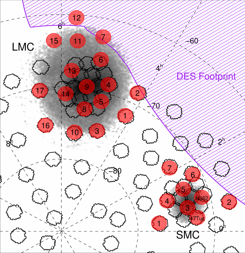
Figure 1.— Map of the APOGEE MC fields (red filled symbols) shown on top of the 2MASS red giant branch star density map. The APOGEE MC field names are indicated by the overplotted numbers. Open hexagons (2.2${}^{\circ}~{}$in diameter) with no overplotted numbers designate other fields from the SMASH survey. The DES footprint is shown in the purple shaded region. An equatorial $\alpha$/$\delta$ grid is marked by dashed lines.

Fortunately, the Apache Point Observatory Galactic Evolution Experiment (APOGEE, Majewski et al. 2017), part of SDSS-III (Eisenstein et al., 2011) and SDSS-IV (Blanton et al., 2017), through installation of a second APOGEE spectrograph (APOGEE-2S; Wilson et al., 2019) on the du Pont telescope at Las Campanas Observatory (LCO), has recently procured high-resolution, $H$-band spectra for already several thousand stars residing in the MCs. These observations cover much of the galaxies: out to 10${}^{\circ}~{}$for the LMC and 6${}^{\circ}~{}$for the SMC, and with large azimuthal coverage for both. An advantage of these particular data is that they can be compared directly to the vast collection of APOGEE spectra similarly obtained and analyzed for both MW stars as well as stars in a sampling of other MW satellites, which ensures that any observed differences in properties found between galactic systems is likely to be real, and not the result of systematic errors between disparate data sets.

In this paper we analyze the [$\alpha$/Fe]–[Fe/H] abundance patterns of red giant branch (RGB) stars in the Magellanic Clouds in order to understand the chemical evolution and SFHs of these galaxies. We probe and place upper-limits on the position of the $\alpha$-element knee in the LMC and SMC, which provides powerful constraints on the early SFEs of these galaxies. In addition, we introduce a new metric, [Fe/H]_α0.15, that can be used to robustly and uniformly measure the position of a galaxy’s $\alpha$-element abundance trendline. The layout of the paper is as follows: Section 2 provides an overview of the APOGEE MC fields and target selection, while section 3 describes the APOGEE observations currently in hand and the data reduction procedures. In Section 4 we detail how we select bona fide MC member stars. Checks on the veracity of the Southern APOGEE data are presented in Section 5. Our main results are described in Section 6, and the relevance and interpretation of our measurements are discussed in Section 7. Finally, our conclusions are summarized in Section 8.

2. Field and Target Selection

In this work we only analyze spectra of MC RGB stars, but the full APOGEE MC survey consists of many astrophysical targets, which we describe here for future APOGEE MC papers to reference. A brief description of the APOGEE MC survey target selection is given in the SDSS-IV targeting paper (Zasowski et al., 2017), but we give more details here. The main goal of the APOGEE MC survey is to study the galactic chemical and kinematical evolution of the Magellanic Clouds, with a particular focus on spatial variations. RGB stars are the majority of the stars in our MC survey. However, a large number of other stellar classes were also chosen to enable a variety of astrophysical studies: massive stars, hot main-sequence stars, asymptotic giant branch (AGB) stars, and post-AGB stars. In addition, stars in the Olsen et al. (2011) metal-poor accreted stream were selected to help ascertain their properties and origin, as were some stars that were previously studied with high-resolution spectra for calibration purposes.

To explore spatial gradients in the MCs, we selected fields that spanned a wide range of radius and position angle (see Figure 1 and Table 1). We required a field to have approximately 50 or more MC RGB candidates for which S/N=100 could be obtained with 9 $\sim$1 hour “visits” in the LMC and 12 visits in the SMC. This produced a maximum radius of $\sim$9.5${}^{\circ}~{}$in the LMC and $\sim$6${}^{\circ}~{}$in the SMC. To aid in the chemical analysis we picked fields that also had deep $ugriz$ photometry from the Survey of the MAgellanic Stellar History (SMASH; Nidever et al., 2017) or the Dark Energy Survey (DES; Dark Energy Survey Collaboration et al., 2016). One of the goals of SMASH is to derive accurate spatially-resolved SFHs to old ages. When this information is combined with the precise APOGEE abundances, simple chemical evolution models can be robustly constrained. At the time of this writing, the SMASH SFHs are still being generated; therefore, we did not use them in our current analysis.

To help target likely Magellanic giant stars, especially blue metal-poor giants that can be heavily contaminated by MW foreground stars, we obtained Washington $M$, $T_{2}$, and DDO51 imaging with the WFI camera on the MPG/ESO-2.2m telescope at La Silla. The data were reduced with the IRAF CCDRED package, and photometric parameters derived with the PHOTRED photometry pipeline (Nidever et al., 2017). Figure 2 shows an example of the ($M$-$T_{2}$, $\Delta$[$M$-$DDO$51]) color-color diagram (top panel; Majewski et al., 2000) that is used to select giant star candidates (red polygon), and shown in the ($M$-$T_{2}$, $M$) CMD as red filled circles (bottom panel). The photometry and giant candidates are used later on during the selection of MC RGB targets (see below).

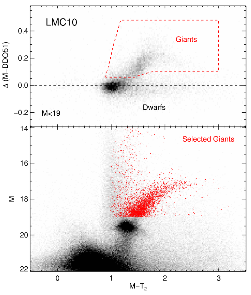
Figure 2.— An illustration of how the Washington $M$, $T_{2}$ and $DDO$51 photometry is used to help select MC RGB targets for field LMC10. (Top) A modified color-color diagram (with the shape of the dwarf locus subtracted from M-$DDO$51) showing the dwarf/giant separation (with $M$ $<$19 mag). The giant selection box is indicated by the red dashed polygon. (Bottom) The color-magnitude diagram with stars falling in the giant selection box shown as red filled circles. The selected stars are dominated by LMC red giant branch and foreground MW halo giants.

While the Washington+$DDO51$ photometry was used to prune out any potential MW foreground dwarfs, the selection of RGB targets otherwise used a wide ($J$-$K_{\rm s}$) range to avoid producing a bias against metal-poor stars as seen in Figure 3. This figure shows the 2MASS photometry of all stars (grayscale) in seven representative LMC fields (with foreground MW sequences identified) with our APOGEE targets in color points to illustrate our targeting strategy. The RGB stars which are used in this analysis are shown as red (bright RGB) and orange (fainter RGB) filled dots, and were selected using the Washington and $DDO$51 photometry.

Initial estimates indicate that there is $\sim$20–40% vignetting in the outer portion of the field of view of the Southern APOGEE fiber plugplates (0.8°$<$$R$$<$0.95°; Wilson et al., 2019). For this reason, most APOGEE-2S fields restrict targets to a field radius of 0.8°. This same restriction was used in the MC fields when there were enough bright targets to fill the fibers allotted to each target class for that field. Exceptions were made for bright but rare targets (e.g., supergiants, main-sequence stars) and RGB targets in outer fields, where the density is low. Note that an initial set of MC targets with a 0.8${}^{\circ}~{}$outer radius for all target types and fields was created and observed in the first APOGEE-2S MC observing run in October 2017. Unfortunately, with the smaller radius restriction a large fraction of intended MC RGB targets were “lost” in the lower density outer fields. For later observing runs the plates were redesigned to include the original targets in the outer radial zones, and observed starting in December 2017. Therefore, some stars will have more visits than the originally planned 9/12 for the LMC/SMC.

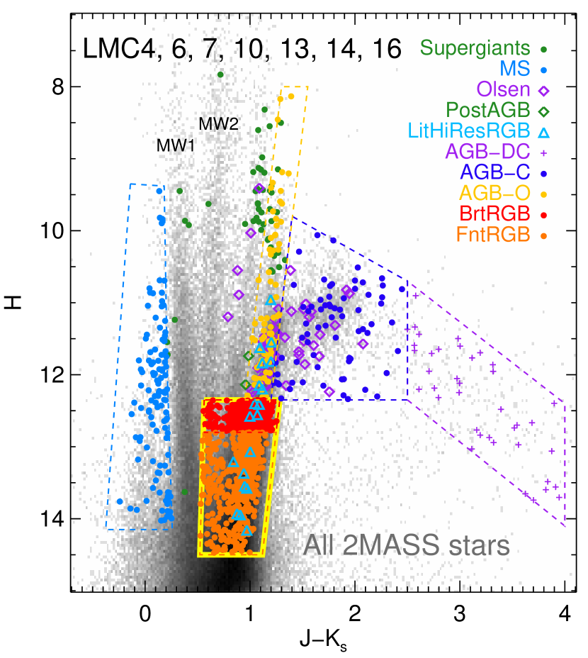
Figure 3.— The 2MASS near-infrared color-magnitude diagram of seven representative LMC fields with the density of all stars shown in grayscale and the APOGEE targets identified by their targeting class. The RGB stars that are the main focus of this analysis are highlighted with a thick yellow polygon. The blue sequence of 2MASS stars at $J-K_{\rm s}$ $\sim$0.3 (MW1) is dominated by foreground Milky Way disk F-K dwarfs and the middle sequence at $J-K_{\rm s}$ $\sim$0.7 (MW2) is dominated by foreground Milky Way disk K dwarfs and halo red clump stars (Nikolaev & Weinberg, 2000).

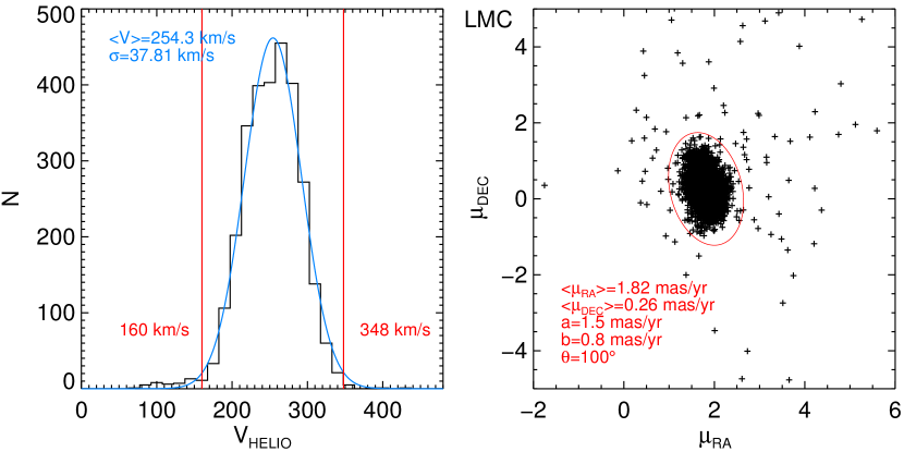
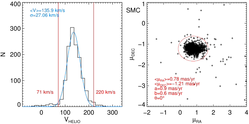
Figure 4.— The distribution of heliocentric radial velocities (left) and Gaia DR2 proper (right) motions of APOGEE RGB targets in the LMC (top) and SMC (bottom) fields. The applied velocity cuts to remove MW contamination

are shown in the red lines (for radial velocity) and ellipses (proper motions). The cuts remove 4% and 8% of the LMC and SMC RGB sample, respectively.

The target selection for each MC field proceeds as follows. All targets are selected for each class according to the criteria described in the list below. An absolute priority is given for all targets in the full list in a two-step process using first the “group priority” (the priority of one group of targets to each other; in the order listed below), and then by the priority within the group using a sorting algorithm (none, random, magnitude, or CMD-uniform). Next, a limit on the number of targets for each class that can be assigned fibers is imposed, with a 50% excess as a buffer for dealing with fiber collisions and other contingencies. Targets with bright neighbors (brighter than 2 mag and within 6″) and targets that collide with a higher priority targets within 56″ (the minimum allowed fiber-to-fiber spacing; Zasowski et al. 2013) are removed. Any extra targets above the limit for that class are removed. In addition, the total number of targets for that entire field (250 for MC fields and 205 for the NGC362 and 47 Tucanae calibration-cluster fields) is imposed and any excess targets are removed from the low priority end of the list. Finally, the list of targets and their information, as well as the selection function fraction (the number of targets selected divided by the total number in that class) are saved. Unlike the standard APOGEE observing for deep fields, where a “cohorting” scheme is utilized to allow swapping of brighter targets from field visit to field visit to increase the number of targets observed (Zasowski et al., 2013), for the MC observing the same targets are observed for the full number of visits each field is visited. The MC target selection software is available at https://svn.sdss.org/public/repo/apogee/apogeetarget/trunk/pro/mcs/

Details on how the ten target classes were selected are given below (in target-class priority order):

1. Supergiants: Massive Magellanic stars were selected from Neugent et al. (2012) and Bonanos et al. (2009), and combined in one catalog. Blue stars that overlap the “main-sequence” target class (see below) were removed. Generally a maximum of 20 fibers per field (but increased to $\sim$35 in some inner fields) were allotted for the supergiants, and a limiting radius of 0.95${}^{\circ}~{}$was used to improve the yield.

2. Main-sequence: Young, blue main-sequence targets were selected using the cyan box in the ($J$-$K_{\rm s}$, $H$) diagram, and are shown as filled light blue circles in Figure 3. Roughly 20 fibers per field were allotted for the main-sequence stars, and the stars were selected with magnitude priority sorting and a limiting field radius of 0.95°.

3. Olsen stream: Olsen et al. (2011) discovered a stream of metal-poor stars in the LMC that might be accreted SMC stars. A maximum of 20 fibers per field were allotted for the Olsen stream stars and these were selected with magnitude priority sorting and a limiting field radius of 0.95°.

   

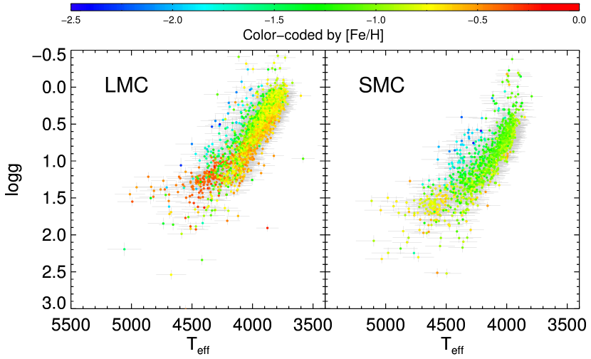
   Figure 5.— The distribution of the selected MC RGB stars in $\rm T_{eff}$ – $\log{g}$ space, and color-coded by [Fe/H] for stars with no ASPCAP STARBAD flag set.

4. Post-AGB: Cool post-AGB stars were selected from Kamath et al. (2014, 2015). A maximum of 10 fibers per field were allotted for the post-AGB stars and these were selected with random priority sorting and a limiting field radius of 0.80°.

5. Literature High-resolution RGB: To check our results, we observed RGB stars that other groups have also studied with high-resolution spectra (Van der Swaelmen et al. 2013 and Carrera et al., in prep). A maximum of 10 fibers per field were allotted for the literature RGB stars, and these were selected with magnitude priority sorting and a limiting radius of 0.80${}^{\circ}~{}$. Some of the literature targets are shown as blue open diamonds in Figure 3. To date, 24 literature RGB stars have been observed, but only 1 star has sufficient S/N for reliable abundances. A meaningful comparison cannot be performed at this time.

6. AGB-DC: The AGB targeting strategy was guided by the AGB selections in Nikolaev & Weinberg (2000) using 2MASS (Skrutskie et al., 2006), and Dell’Agli et al. (2015b, a) using $Spitzer$. A maximum of 15 fibers per field were allotted to dusty carbon-rich AGB stars. These targets were selected using the magenta box in the ($J$-$K_{\rm s}$, $H$) diagram, using a “CMD-uniform” sampling designed to select stars uniformly across the 2-D CMD space. These targets were also selected with a limiting field radius of 0.80°. Some of the AGB-DC targets observed to date are shown as filled magenta crosses in Figure 3.

7. AGB-C: A maximum of 15 fibers per field were allotted to carbon-rich AGB stars, and the targets were selected using the blue box in the ($J$-$K_{\rm s}$, $H$) diagram with CMD-uniform sampling and a limiting field radius of 0.80°. The AGB-C targets are shown as filled blue circles in Figure 3.

8. AGB-O: Oxygen-rich AGB stars were assigned to a maximum of 15 fibers per field (but this was increased to $\sim$40 in some inner regions). These targets were selected using the yellow box in the ($J$-$K_{\rm s}$, $H$) diagram with CMD-uniform sampling and a limiting field radius of 0.80${}^{\circ}~{}$(except for the field SMC7 which used 0.95°). Some of the AGB-O targets are shown as filled yellow circles in Figure 3.

9. Bright RGB: The largest group of targets are the red giant branch stars, selected in two groups – “bright” and “faint” (see below). The higher priority group are those for which S/N=100 spectra will be obtained in 9/12 visits for the LMC/SMC. Targets were selected from among those that passed the Washington photometry giant star selection (see above and Figure 2) and that lie within the red-bounded polygonal area in the ($J$-$K_{\rm s}$, $H$) diagram. The RGB CMD selection box extends to fairly blue colors ($\sim$0.55) to ensure we capture metal-poor MC stars at the risk of some contamination from metal-poor MW halo stars (Nikolaev & Weinberg, 2000). These stars span a magnitude range of 12.35$<$$H$$<$12.8 for the LMC and 12.9$<$$H$$<$13.2 for the SMC. Random sampling and a limiting field radius of 0.80${}^{\circ}~{}$(except for some outer fields where 0.95°was allowed) were used for the selection. All of the unassigned fibers remaining after attempting to fill them with stars in any of the above target classes were allotted to bright RGB stars, up to a maximum of 250. The bright RGB targets are shown as filled red circles in Figure 3. Thus far, 2505 bright RGB targets have been observed, with 2374 having S/N$>$40.

10. Faint RGB: Faint RGB stars were targeted if not enough bright RGB targets were available. Targets were selected from among those that passed the Washington photometry giant cut and that lie within the orange polygon in the ($J$-$K_{\rm s}$, $H$) diagram. Magnitude priority sorting and a limiting field radius of 0.80${}^{\circ}~{}$(except for some outer fields that used 0.95°) were adopted. All of the remaining fibers were allotted up to a maximum of 250. The faint RGB targets are shown as filled orange circles in Figure 3. Thus far, 2061 faint RGB targets have been observed, with 1490 having S/N$>$40.

The CMDs were not dereddened for the target selection, because it is challenging to calculate accurate star-by-star extinctions in the inner MCs (but see Choi et al. 2018a). However, our CMD selection polygons were made large enough to capture the relevant stellar populations, even with the moderate reddening seen in the NIR. For the SMC fields, the CMD selection polygons were shifted in magnitude by +0.4 mag due to the larger SMC distance compared to that of the LMC.

The selection of targets in the 30 Dor “APOGEE-2S first light” plate was focused on getting spectra for massive stars, and so used different criteria than used for the normal MC fields. A number of massive star types (e.g., Luminous Blue Variables, Wolf-Rayet, Blue Supergiant, main-sequence stars) were selected manually from existing catalogs, and will be discussed in full in a subsequent paper (Stringfellow et al., in preparation). In addition, 72 RGB stars were selected from the CMD in a manner similar to that shown in Figure 3, but with a magnitude range of 12.30$<$$H$$<$13.0, and a less expansive blue limit of $J-K_{\rm s}$=0.9.

3. Observations and Reductions

For the last seven years, the original APOGEE instrument (Wilson et al., 2019) has been taking data of the Northern sky using the SDSS-2.5m telescope (Gunn et al., 2006) at Apache Point Observatory. However, to allow the APOGEE-2 project to access the entire Milky Way, as well as the Magellanic Clouds, a Southern copy of the APOGEE instrument (Wilson et al., 2019), was installed at the du Pont-2.5m telescope at LCO in January 2017, with first light on February 16, 2017, using the 30 Dor plate. The Southern instrument is nearly identical to the Northern one, with some small modifications, such as a revised LN₂ tank suspension system and protections against seismic events (APOGEE-2S; Wilson et al., 2019). APOGEE-2S uses 300 fibers and plugplates with a 2${}^{\circ}~{}$diameter field-of-view.

Since the inaugural “first light” observations of the 30 Doradus plate, the first full season featuring Magellanic Cloud targeting began in September 2017 and are continuing. We present data from the 16th SDSS data release (DR16), which includes data taken through August 31, 2018, which will be released in December 2019 and described in detail by Jönsson et al. (in prep.). These data were reduced through the standard APOGEE reduction pipeline (Nidever et al., 2015), and stellar parameters and abundances were obtained via the ASPCAP pipeline (Holtzman et al., 2015; García Pérez et al., 2016), which uses a library of synthetic spectra (Zamora et al., 2015). ASPCAP first derives stellar parameters by fitting to a 7-D synthetic spectral grid ($\rm T_{eff}$ , $\log{g}$ , [M/H], [$\alpha$/M] (O, Mg, Si, S, Ca, Ti), [C/M], [N/M], and $v_{\rm micro}$), and then derives individual element abundances (C, C I, N, O, Na, Mg, Al, Si, P, S, K, Ca, Ti, Ti II, V, Cr, Mn, Fe, Co, Ni, Cu, Ge, Rb, Yb, Ce, and Nd) by fitting spectral “windows” that are sensitive to variations in those individual element abundances. Changes since DR14 (Abolfathi et al., 2018) include improvements to the linelist, the use of MARCS atmospheres (Gustafsson et al., 2008) for all grids, no internal temperature-dependent abundance calibrations were applied, and improved derivation of uncertainties. Constant abundance offsets were determined from the mean offset of solar metallicity stars in the solar neighborhood from solar abundance ratios. The additive offsets for the elements relevant to this study are 0.009, 0.038, 0.002, 0.000, and 0.033 dex for Mg, Si, Ca, Fe and $\alpha$, respectively. For our analysis, only stars that had reliable stellar parameters (no bad quality flags set) were used. Statistical uncertainties are derived by looking at repeat observations of stars in different overlapping fields or with different visits and then fitting the logarithm of the scatter as a linear function of $\rm T_{eff}$, [M/H], and S/N. It is possible that the uncertainties are somewhat underestimated. We conservatively increase our uncertainties to match the intrinsic abundance scatter of first generation stars in globular clusters which effectively acts as an upper limit to our actual uncertainties. The factors are 1.5$\times$, 1.7$\times$ and 2.7$\times$ for [Mg/Fe], [Si/Fe] and [Fe/H], respectively, while [$\alpha$/Fe] and [Ca/Fe] do not need to be adjusted. Because this is the first paper to utilize data from the Southern spectrograph, in Section §5 we perform quality checks of the stellar parameters and abundances to verify the reliability of their results.

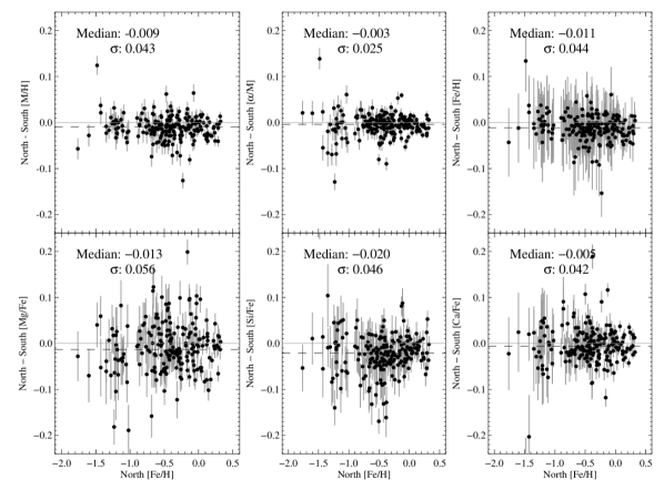
Figure 6.— Comparisons of the derived abundances for 203 stars observed from both the Northern and Southern telescopes. Medians and standard deviations of the abundance differences are indicated in each panel.

4. Selection of Magellanic Cloud Member Stars

While steps were taken to try to select as many MC RGB stars as possible (e.g., selection using the Washington photometry), it is likely that we have some MW contamination in the APOGEE MC fields, especially from MW halo stars. To refine our analysis sample from those stars that were observed, we use ASPCAP stellar parameters, radial velocity, and Gaia DR2 (Brown et al., 2018) proper motions (unavailable when the target selection was made) to select bona fide MC RGB stars. To this end, we required reliable stellar parameters for all the stars from the ASPCAP pipeline and $\rm T_{eff}$ $<$5200 K and $\log{g}$ $<$ 3.4. The RV and proper motion selections are shown in Figure 4. A Gaussian fit to the LMC RV distribution yields a mean of 254.3 km s${}^{-1}~{}$with $\sigma_{\rm V}$=37.8 km s^-1, and we use lower/upper thresholds of 160/348 km s^-1, which are roughly $\pm$2.5$\sigma$. The same values for the SMC are mean/$\sigma_{\rm V}$=135.9/27.1 km s${}^{-1}~{}$with lower/upper thresholds of 71/220 km s^-1. Ellipses with the parameters, determined by eye, and shown in Figure 4, are used for the proper motion cuts. Of the 2897/1363 LMC/SMC stars with S/N$\geq$20, 122/121 are pruned with the velocity cuts, or 4%/9% of the samples. Figure 5 shows the $\rm T_{eff}$–$\log{g}$ distribution of the final LMC and SMC RGB samples color-coded by metallicity. Our selection is higher up the giant branch than Van der Swaelmen et al. (2013) and Lapenna et al. (2012) studies, but includes large portions of the giant branch. Table 1 gives information on all our fields and MC targets.

5. Quality Checks of APOGEE-S data

This work is among the first to utilize data from the Southern Hemisphere component of APOGEE-2. Therefore, we perform a number of quality checks to verify the reliability of the spectroscopic parameters:

• Comparison of abundances between stars observed from both the Northern and Southern APOGEE spectrographs.

• Comparison of the APOGEE cluster abundances to the optical cluster abundances of Carretta et al. (2009a, b).

• Comparison of the APOGEE abundances to the abundances from GALAH DR2 (Buder et al., 2018).

• Comparison of APOGEE ASPCAP abundances to abundances derived from APOGEE spectra in a semi-independent way using BACCHUS (Masseron et al., 2016).

5.1. Comparison of APOGEE-2N and APOGEE-2S

First, we compare the derived abundances for APOGEE stars observed from both the Northern and Southern telescopes (none from the MC fields). We select overlap stars that have similar effective temperatures to the LMC (3750–4500 K) and S/N $>$ 70 from both spectrographs. The 203 stars that satisfy these criteria are shown in Figure 6. We find that the abundances agree within the reported uncertainties with no obvious trends in [Fe/H], but find that there is a small offset in [Si/Fe] of $\sim$ 0.02 dex.

While the abundance comparisons across telescopes appear reasonable, the overlap sample has only a few stars with [Fe/H] $<$ $-$1.5. Therefore, it is also important to verify the quality of the spectra of the most metal-poor stars of our sample, as they drive our ability to measure the $\alpha$-poor knee. In the top panel of Figure 7, we show the spectral features of Fe, Mg, and Si for 5 LMC stars with $-$2.5 $<$ [Fe/H] $<$ $-$2.0. This illustrates that there are plenty of measurable features in these southern spectra that are fit well by ASPCAP, and brings confidence that these are really metal-poor, $\alpha$-enhanced stars. In addition, the bottom panel of Figure 7 shows how the strengths of the Mg and Si lines vary with $\alpha$-abundance for one metal-poor APOGEE star. Therefore, this indicates that APOGEE spectra are sensitive to $\alpha$ abundance even for these metal-poor stars.

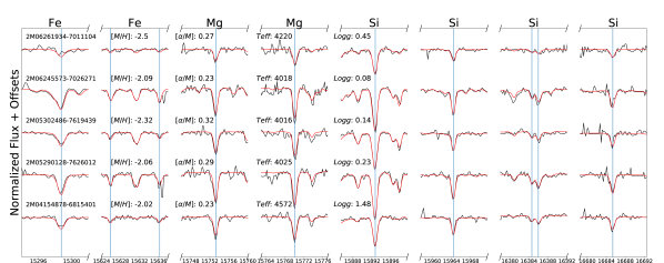
Figure 7.— (Top) The most prominent abundance features of Fe, Mg and Si in 5 example metal-poor LMC stars (black) and the best-fitting ASPCAP synthetic spectrum (red). The central wavelengths of the lines are indicated by vertical blue lines. (Bottom) An example of a metal poor APOGEE DR16 spectrum focused on the most prominent Si and Mg lines indicating how they vary in strength with $\alpha$-abundance. The APOGEE spectrum is shown in black, the best-fitting ASPCAP synthetic spectrum in orange, and synthetic spectra enhanced and depleted by 0.2 dex in [$\alpha$/M] (relative to the best-fitting parameters) shown in green and blue, respectively.

5.2. Cluster Abundances

In addition, we compare the APOGEE metallicities of 26 globular clusters (15 from the South and 11 from the North) with measurements from Carretta et al. (2009a) and Mészáros et al. (2013) external globular cluster data. The differences in the mean metallicities are shown in Figure 8. For each of these clusters, we select members using spatial and radial velocity cuts, and compute the reported mean [Fe/H] for each cluster and standard error of the mean from first-generation globular cluster members (defined as [Al/Fe] $<$ $+$0.4) with relatively high S/N ($>70$), $3700<T_{\rm eff}<5500$K, and that are not flagged with poor spectra or stellar parameters. The metallicities agree fairly well even to low metallicities, with a slight 0.06 dex offset between the two sets of measurements (APOGEE is more metal-rich than Carretta et al.). This agrees largely with Mészáros et al. (2013, using DR10 data), and Masseron et al. (2019, using DR14 data) although we find that the DR16 metallicities of the most metal-poor globular clusters (M92 and M15) agree better with optical studies than the previous APOGEE metallicities.

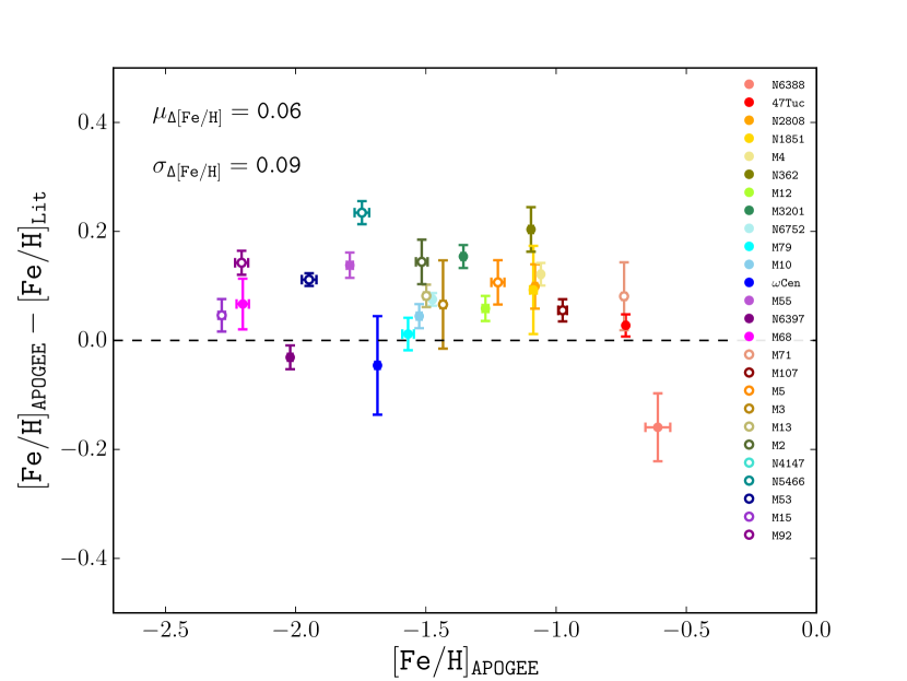
Figure 8.— A comparison of the mean [Fe/H] of the APOGEE-2 globular clusters observations (using first-generation globular cluster stars as described in the text) with Southern clusters (filled points) from Carretta et al. (2009a) and Northern clusters (empty points) compiled by Mészáros et al. (2013). While there are some deviations (e.g., NGC6388 and NGC6397) the measurements show an offset of 0.06 dex, with a scatter of 0.09 dex.

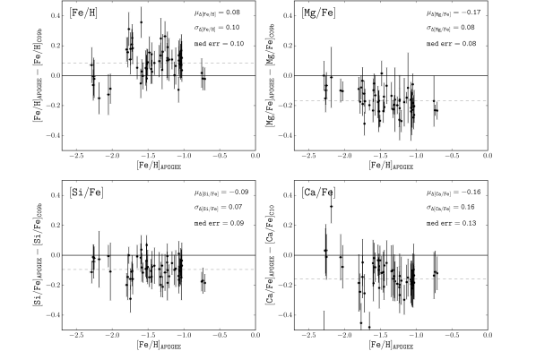
Figure 9.— A comparison of the abundances ([Fe/H], [Mg/Fe], [Si/Fe] and [Ca/Fe]) from (Carretta et al., 2009b) for first-generation globular cluster stars in 11 southern globular clusters. The scatter in the abundance measurements are consistent with the uncertainties but we see offsets of $+$0.08 dex in [Fe/H], $-$0.17 dex in [Mg/Fe], $-$0.09 dex in [Si/Fe], and $-$0.16 dex in [Ca/Fe].

Figure 10.— The APOGEE DR16 [$\alpha$/Fe] versus [Fe/H] distributions of first generation stars ([Al/Fe]$<$0.4) of ten globular clusters. While these cluster stars showed some anti-correlation of [$\alpha$/M] with [M/H] in Mészáros et al. (2013) for DR14, the removal of the second generation stars and using abundances relative to Fe essentially removes any correlation and gives small scatters.

Figure 9 compares individual [Fe/H], [Mg/Fe], [Si/Fe], and [Ca/Fe] of 58 individual first-generation giants ([Al/Fe] $<0.4$) in 11 Southern globular clusters observed by APOGEE to those measured by Carretta et al. (2009b), using the same cuts on S/N, effective temperature, and flags employed to compare mean globular cluster metallicity above. The scatter in the abundance differences are consistent with the measurement uncertainties, however there are offsets (across a wide range of metallicity) of $+$0.08 dex in [Fe/H] (consistent with the mean metallicity comparison), $-$0.17 dex in [Mg/Fe], $-$0.09 dex in [Si/Fe], and $-$0.16 in [Ca/Fe].

Mészáros et al. (2013) showed the APOGEE DR10 [$\alpha$/M] versus [M/H] distributions of stars from ten globular cluster and found there to be a correlation between [$\alpha$/M] and [M/H] (see their Figure 12). This correlation still exists in DR16 but at a lower level. The correlation is likely due to the fact that at low metallicities the [M/H] of second generation stars (which have high [Al/Fe]) is dominated by strong Al lines which pushes the [M/H] to higher values than those of their first generation (and low [Al/Fe]) counterparts. As the second generation stars also have lower $\alpha$-abundances then the first generation stars, this effect causes a correlation between [$\alpha$/M] and [M/H]. The anti-correlation is mostly removed by using abundances relative to Fe rather than M, but not entirely. The removal of the “problematic” second generation stars essentially eliminates the anti-correlation issue. Figure 10 shows the APOGEE DR16 abundances of first generation stars of the same ten Meszaros et al. globular clusters (relative to Fe). No anticorrelation is apparent and the scatters are small. We note that the LMC stars have low [Al/Fe] and do not suffer from the globular cluster second generation star antic-correlation effect.

5.3. Comparison to GALAH DR2

Figure 11 shows a similar comparison of the APOGEE-2S data with MW giant stars also observed by GALAH DR2 (Buder et al., 2018). The selected stars have S/N$>$60 in both surveys, $\rm T_{eff}$ $<$5000K, $\log{g}$ $<$3.9, no STARBAD flag set in APOGEE, and cannon_flag=0 and flag_X_fe=0 for GALAH, as recommended by Buder et al.. The stellar parameters span a range of 3900$<$$\rm T_{eff}$$<$5000K, 0.8$<$$\log{g}$$<$3.9, and $-$2.1$<$[Fe/H]$<$ $+$0.3. The largest difference is the offset of approximately $-$0.2 dex in [Fe/H] at the metal-poor end ([Fe/H] $<$ $-$1.0). This is opposite in direction of the smaller offset seen between APOGEE and Carretta et al. (2009a) in Figures 8 and 9. GALAH silicon and calcium show slight offsets at the $\sim$0.05 dex level, but the scatter is consistent with the measurement uncertainties. The [Si/Fe] offset is consistent with the one seen when comparing APOGEE and Carretta et al., but smaller in magnitude. The magnesium abundance offset is small, but in the opposite sense of the Carretta et al. comparison.

Based on these comparisons, the largest discrepancies are the [Mg/Fe] offset with Carretta et al. and the low-metallicity offset in [Fe/H] with GALAH. However, we find that these offsets are opposite in sign across the two optical samples. Furthermore, Jönsson et al. (2018) found that magnesium was the most reliable APOGEE abundance element in DR14, with no offset and a scatter of 0.09 dex, when comparing to an optical study and constrained to [Fe/H] $>$ $-$1. There might be small offsets in the APOGEE [Si/Fe] and [Ca/Fe] abundances, on the order of $\sim$0.05 dex, which would push the APOGEE $\alpha$-element abundance trends higher.

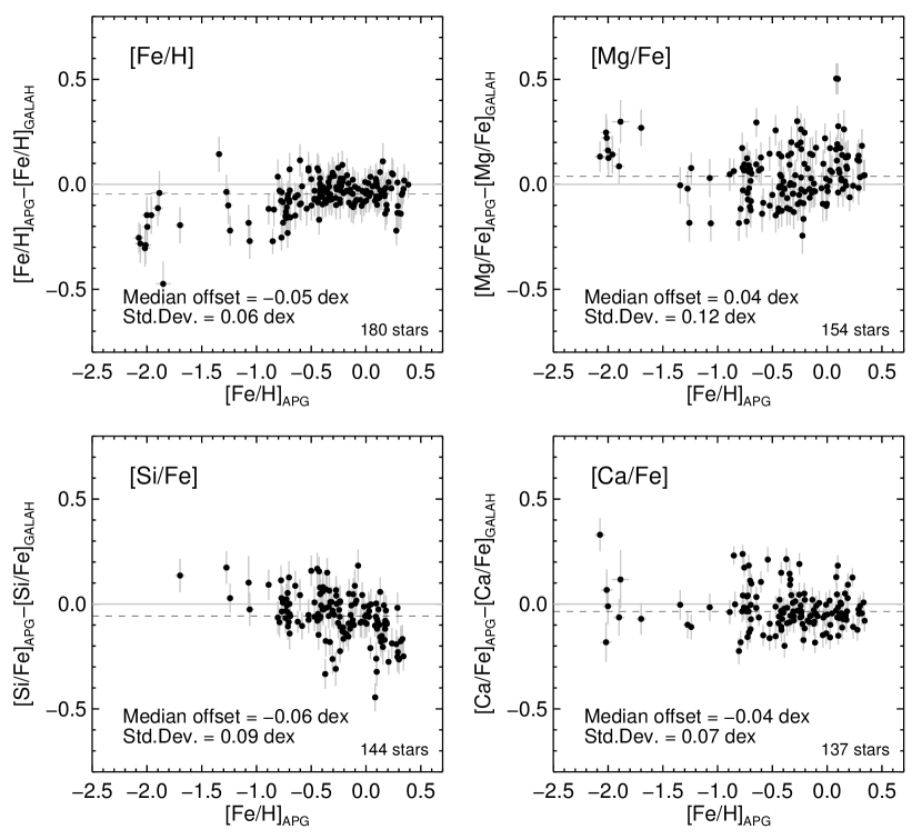
Figure 11.— A comparison of the abundances from the GALAH survey and the APOGEE-2S stars for [Fe/H], [Mg/Fe], [Si/Fe] and [Ca/Fe]. We select stars with S/N$>$60 in each survey, $\rm T_{eff}$ $<$ 5000, no STARBAD flag set in APOGEE, and cannon_flag=0 and flag_X_fe=0 for GALAH as recommended by Buder et al. (2018). Offsets and standard deviations are indicated in each panel.

5.4. BACCHUS Analysis

We further check the ASPCAP $\alpha$-element abundances by completing a semi-independent stellar-abundance analysis of $\sim$90 stars randomly selected from the LMC sample, but ensuring good coverage of the metal-poor stars, and a comparable number of stars randomly selected from Milky Way field population observed with APOGEE. The abundance analysis was carried out using the Brussels Automatic Code for Characterizing High accUracy Spectra (BACCHUS, Masseron et al., 2016). The BACCHUS analysis is “semi-independent” in that some stellar parameters (listed below) are fixed to the ASPCAP values. However, BACCHUS uses a more select list of lines to derive Fe and $\alpha$-element abundances, and generates new, self-consistent (in the abundances) synthetic spectra during the fitting process, in contrast to ASPCAP, which interpolates in a large-dimensional grid.

The current version of BACCHUS makes use of the the MARCS model atmosphere grid (Gustafsson et al., 2008), and the radiative transfer code TURBOSPECTRUM (Alvarez & Plez, 1998; Plez, 2012) to generate synthetic spectra. The MARCS model atmosphere grid includes both carbon and $\alpha$-element enhancements. Similar to Hawkins et al. (2016), we fix the $\rm T_{eff}$ and $\log{g}$  stellar atmospheric parameters to the best-fit values from the ASPCAP pipeline (i.e., the uncalibrated values of $\rm T_{eff}$and $\log{g}$ , which can be found in the FPARAM column in the ASPCAP results table). In addition to $\rm T_{eff}$ and $\log{g}$ , we also fix the C and N values to those found in the best fit from the ASCAP pipeline. The [Fe/H] and microturbulent velocity were then determined using the same procedure as in Hawkins et al. (2016). In short, microturblence was determined by ensuring no correlation between derived Fe abundance and reduced equivalent width (i.e., equivalent width divided by wavelength). The line selection for the various elements is the same as in Hawkins et al. (2016).

After fixing the $\rm T_{eff}$, $\log{g}$ , [C/H], and [N/H], and deriving [Fe/H] and microturbulent velocity, the individual abundances for C, N, O, Mg, Si, Ca, and Ti were derived by using $\chi^{2}$ minimization between the observed spectra and the synthetic spectra. In the top panel of Figure 12, we show the difference of ASPCAP and BACCHUS-derived [Fe/H], as a function of ASPCAP [Fe/H], for the LMC (black circles) as well as a Milky Way comparison sample also observed in the APOGEE-2S survey (blue squares). In the bottom panel of Figure 12, we show the difference of ASPCAP and BACCHUS-derived [Mg+Si+Ca/Fe], as a function of ASPCAP [Fe/H], for the same stars as the top panel. The median offset in [Fe/H] is $-$0.143 dex and $-$0.03 dex in [$\alpha$/Fe] for both the LMC and MW sample. We find that the results from ASPCAP appear to be robust and confirmed with a semi-independent BACCHUS analysis.

6. Results

6.1. $\alpha$-element Abundance Patterns of RGB stars in the Magellanic Clouds

Figure 13 shows the APOGEE ASPCAP parameter-level $\alpha$-element abundance (parameter-level [$\alpha$/M] $+$ parameter-level [M/H] $-$ windowed [Fe/H]) distribution of the MC RGB stars. The parameter-level [$\alpha$/Fe] (upper left), which fits all of the $\alpha$-elements (O, Mg, Si, S, Ca, and Ti) simultaneously (keeping their relative abundances identical) in ASPCAP’s 7-D synthetic grid parameter fitting, is more accurate than the individual $\alpha$-elements, but somewhat more challenging to interpret because the relative “weight” of different $\alpha$-elements changes with metallicity and $\rm T_{eff}$. Therefore, we compare the parameter-level [$\alpha$/Fe] to the windowed [Mg/Fe], [Fe/Si], and [Ca/Fe] abundances, shown in the other panels. These $\alpha$-elements exhibit qualitatively similar abundance patterns to the parameter-level [$\alpha$/Fe], although with some small differences and offsets. The general pattern seen in all four panels is that the LMC $\alpha$-element abundances are quite flat in metallicity from [Fe/H]=$-$1.7 to $-$0.3. There is a slight increase in $\alpha$ at [Fe/H] $>$ $-$1.0, most clearly seen in the parameter-level [$\alpha$/Fe], [Mg/Fe], and [Si/Fe]. At the metal-poor end the $\alpha$-element abundances increase but do not reach their maximum until the most metal-poor stars at [Fe/H]$\approx$ $-$2.2. Figure 13 also shows both the S/N$>$40 stars (black) and S/N$>$70 stars separately. The two sets of stars exhibit nearly identical abundance patterns; this illustrates the reliability of the individual element $\alpha$-element abundances down to S/N=40, although perhaps slightly less so for Ca at the lowest metallicities.

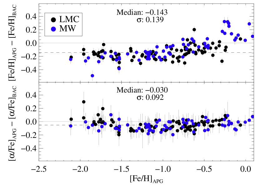
Figure 12.— (Top) The difference of ASPCAP minus BACCHUS-derived [Fe/H] as a function of ASPCAP [Fe/H] for $\sim$90 LMC (black circles), and MW (blue square) stars both observed from APOGEE-2 south. The median offset is $-$0.143 dex with a scatter of 0.139 dex. (Bottom) Same as top panel but for the average [$\alpha$/Fe] ([Mg/Fe], [Ca/Fe], and [Si/Fe]) as a function of metallicity. The median offset is $-$0.030 dex with a scatter of 0.092 dex.

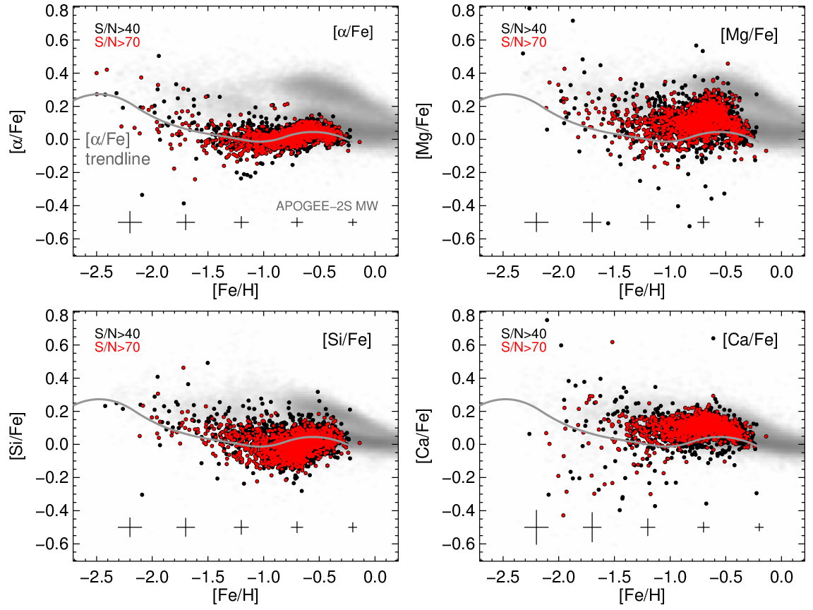
Figure 13.— The $\alpha$ abundances for the APOGEE LMC stars for S/N$>$40 (filled black circles) and S/N$>$70 (red filled circles). The density of APOGEE-2S Milky Way disk field stars with similar $\rm T_{eff}$, $\log{g}$ and S/N as the LMC stars is shown in grayscale for reference. The trendline of the parameter-level [$\alpha$/Fe] (upper-left panel) is shown in each panel as a fiducial. At the bottom of each panel are median ASPCAP errors bars for the S/N$>$40 sample

.

Now that we have verified that the parameter-level [$\alpha$/Fe] values yield abundance patterns consistent with those of the individual $\alpha$-elements and are reliable to low S/N, henceforth we use the more precise parameter-level [$\alpha$/Fe]. In the top two panels of Figure 14 we show the $\alpha$-element abundance distribution of both the LMC and SMC in comparison to those for MW stars, and in the bottom two panels we compare our MC data to other dwarf galaxies abundance data from the literature.

Both the APOGEE MC and MW stars come from the Southern APOGEE instrument. While both MCs differ from the MW, in that they are generally more $\alpha$-poor at fixed [Fe/H], the MCs also differ from each other. We find that the LMC reaches metallicities as high as [Fe/H]$\approx$ $-$0.2, whereas the SMC is only as metal-rich as [Fe/H] $\approx$ $-$0.5. We also appear to be lacking the most metal-poor stars in our SMC sample, likely due to the (current) lower S/N in the SMC sample compared to the LMC, because the stars are $\sim$0.4 mag fainter. However, we are able to measure the increase in [$\alpha$/Fe] (with decreasing [Fe/H]) and constrain the $\alpha$-knee in both the LMC and SMC to [Fe/H] $\sim$ $-$2.2. Although there is no clear evidence yet of a high-$\alpha$ plateau in either galaxies.

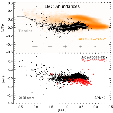
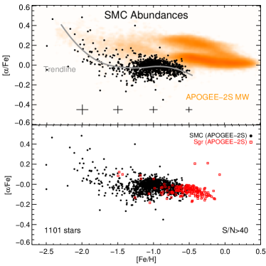
Figure 14.— The $\alpha$ abundances of the Magellanic Clouds ([$\alpha$/Fe] vs. [Fe/H]). (Left) LMC and (Right) SMC with the APOGEE MC as black filled circles. (Top) The density of APOGEE-2S MW stars (orange), and a B-spline trendline for the MC stars (gray). (Bottom) comparison of the LMC/SMC to Sagittarius (APOGEE-2S, open red squares). Median uncertainties from ASPCAP are shown in the top panels.

In the bottom two panels of Figure 14 we show the $\alpha$-element abundance distributions of the MCs as compared to other MC spectroscopic samples: individual stars from Van der Swaelmen et al. (2013, purple diamonds) and individual cluster stars as compiled in Sakari et al. (2017, blue crosses). They agree reasonably well with the APOGEE results at higher metallicities, but the Van der Swaelmen et al. sample does not cover the low-metallicity region as our data. The Van der Swaelmen et al. stars do seem to contain a larger fraction of $\alpha$-element enhanced LMC stars than the APOGEE sample. We find that the APOGEE stars largely follow a tight sequence in [$\alpha$/Fe]-[Fe/H] space, with only a few stars scattering to super-solar $\alpha$-element abundance. This discrepancy could be due to the fact that the Van der Swaelmen et al. stars are at the center of the LMC, with half of their stars belonging to the bar. In our APOGEE sample, we have only a small fraction of stars that overlap spatially with the Van der Swaelmen et al. sample, and likely have (relatively) very few bar stars. We further discuss the comparison of our APOGEE abundances of the LMC with literature values below in §6.2.

$\begin{array}[]{cc}\includegraphics[width=216.81pt,angle={0}]{lmc_cmd_youngmetalrich_dr16beta.pdf}&\includegraphics[width=216.81pt,angle={0}]{lmc_alphafefeh_youngmetalrich_dr16beta.pdf}\end{array}$

Figure 15.— The young metal-rich, blue LMC population. (Left) The color-magnitude diagram of all the APOGEE-selected LMC stars. The inner fields ($R$ $<$4.8°) are shown as larger symbols and are color-coded by [Fe/H]. The gray polygon more or less selects the inner, metal-rich blue stars. (Right) The [$\alpha$/Fe] vs. [Fe/H] abundances for the high-S/N (greater than 50) LMC stars, with the stars selected in the left panel marked as red filled dots. These stars are predominantly metal-rich, and include the most metal-rich stars in the LMC sample. Of the 125 LMC stars with [Fe/H]$>$ $-$0.30, 90 of them are in this young population (72%), and a significant fraction of the rest are just redward of the selection box. This supports the notion that the most metal-rich population are young (blue-loop) stars in the inner region of the LMC.

The abundances for Fornax from Hendricks et al. (2014, shown as green crosses in the bottom two panels of Figure 14) have a plateau at slightly higher metallicity than that for the LMC. The APOGEE-2S Sagittarius (Sgr) sample (shown as red open squares in Figure 14) exhibits sub-solar $\alpha$-element abundances that have been interpreted as being due to a top-light IMF (Hasselquist et al., 2017). We do not measure the position of the metal-poor knee in the Sgr data, but literature works find a knee in the range of $-$1.5 $\lesssim$ [Fe/H] $\lesssim$ $-$1.2 (de Boer et al., 2014; Carlin et al., 2018), all more metal-rich than the LMC, even though these galaxies were thought to once have similar stellar mass and have both enriched themselves to [Fe/H]$\approx$0.0.

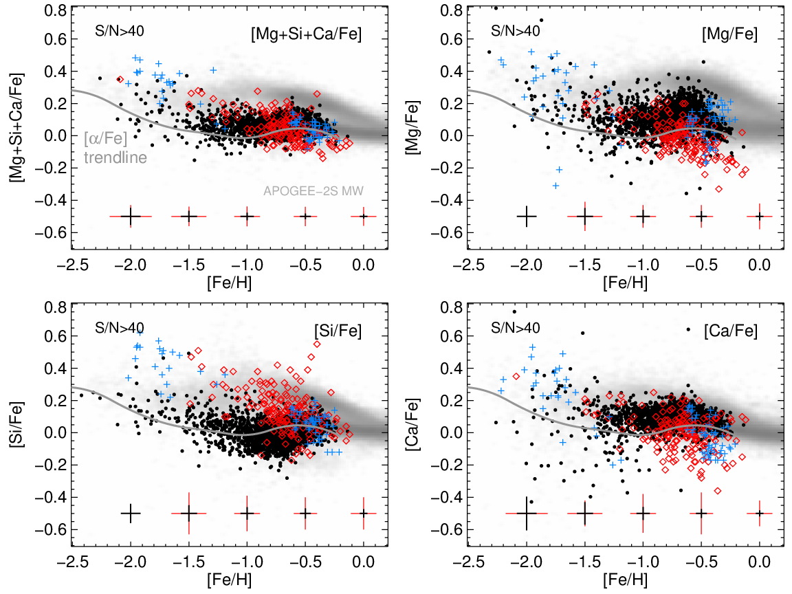
Figure 16.— A comparison of the $\alpha$-element abundances for the APOGEE LMC stars (filled black circles) to those of Van der Swaelmen et al. (2013) (open red diamonds) and LMC clusters (blue crosses; compiled by Sakari et al., 2017). The APOGEE-2S MW distribution for each element is shown in the grayscale in the background for reference. At the bottom of each panel the APOGEE abundance uncertainties are shown in black and the Van der Swaelmen et al. uncertainties in red.

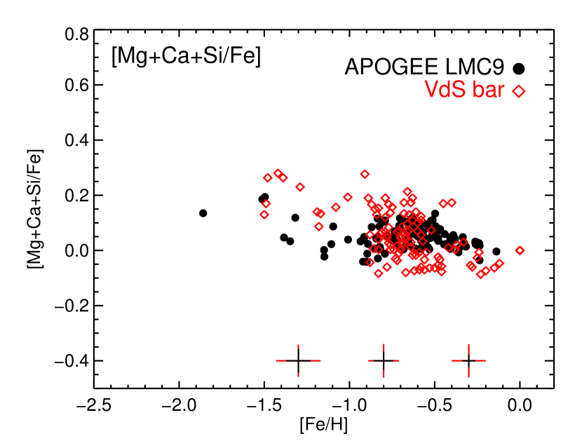
Figure 17.— A comparison of the $\alpha$-element abundances ([Mg+Ca+Si/Fe]) of 129 APOGEE LMC stars with S/N$>$40 in the central field LMC9 (filled black circles) to the 113 “bar” field stars from Van der Swaelmen et al. (2013) (open red diamonds). The distributions of the two samples are very similar with only a slight offset in $\alpha$-abundance of $\sim$0.1 dex at the metal-poor end.

Additionally, we see a rise in $\alpha$-element abundance with metallicity in the LMC, beginning at [Fe/H] = $-$1.0. This implies that after the turn on of Type Ia SNe in the LMC, which lowered the [$\alpha$/Fe] abundance to near-solar at [Fe/H] = $-$1.5, the LMC may have experienced an increase in the number of Type II SNe that were able to enrich the ISM with $\alpha$-elements. An increase in the Type II SNe can be due to a starburst, where the LMC quickly begins to form stars at a much faster rate. We also observe a slight turnover in [$\alpha$/Fe] at [Fe/H] $\sim$ $-$0.5, which could be a sign of the Type Ia SNe exploding from the stars formed at the beginning of the starburst, adding Fe to the ISM of the LMC at the exclusion of the $\alpha$-elements. We further explore this starburst scenario in §6.3.

The SMC does not exhibit an increase of [$\alpha$/Fe] with increasing [Fe/H] beyond the apparent knee position, but it does exhibit a flat pattern starting at [Fe/H] $\sim$ $-$1.5, with perhaps a slight decrease beginning at [Fe/H] $\sim$ $-$0.7. Flat $\alpha$-element abundance patterns can also be indicative of a starburst, or series of starbursts, but these starbursts are not sufficiently powerful to substantially enrich the gas already present with $\alpha$-elements (e.g., Hendricks et al. 2014).

Because of our blue color-cut, applied in order to prevent a metallicity bias in our LMC RGB sample, we have also serendipitously observed young blue-loop, metal-rich stars, as identified in the CMD in Figure 15 (left panel). While a detailed analysis of the reliability of the blue-loop abundances is beyond the scope of this paper, these stars appear to be among the most metal-rich stars in the sample. This fits the scenario where the LMC is currently forming stars (in the inner regions where we observe these blue-loop stars) at a metallicity of [Fe/H] = $-$0.3.

6.2. Comparison to Previous LMC Studies

Previous $\alpha$-element abundance studies of the LMC (e.g., Smith et al., 2000; Pompéia et al., 2008; Lapenna et al., 2012; Van der Swaelmen et al., 2013; Sakari et al., 2017) did not find the relatively flat $\alpha$-element distribution at [Fe/H] $>$ $-$1.0, or the metal-poor $\alpha$-knee that we constrain with our APOGEE dataset. To further investigate this discrepancy, Figure 16 shows a comparison of the APOGEE LMC $\alpha$-element abundances with those of Van der Swaelmen et al. (2013), in red open diamonds, and the LMC cluster star abundances compiled by Sakari et al. (2017) in blue crosses. The abundances of all $\alpha$ elements are fairly consistent at the metal-rich end. In addition, the [Ca/Fe] and [Mg/Fe] abundances agree well between the three datasets. The [Si/Fe] abundances are the most disparate with the literature values being higher at the metal-poor end than for APOGEE. As we previously showed in Section 5, our [Si/Fe] abundances compare well to Carretta et al. (2009b), with a constant offset but no trends with metallicity (Figure 9). It is challenging to say which [Si/Fe] abundances are correct in this instance, however we do note that the abundance patterns in APOGEE are more similar to the $\alpha$-element abundance patterns in other elements, whereas the Van der Swaelmen et al. (2013) Si abundances are slightly different from their other $\alpha$-elements. Finally, the abundance trends of the [Mg+Si+Ca/Fe] average values (upper-left panel of Figure 16 are qualitatively quite similar between the three datasets (although the APOGEE metallicities are a bit more metal poor), suggesting that they are reliable.

To make a clearer comparison between our data and that of Van der Swaelmen et al. we plot the [Mg+Ca+Si/Fe] abundances of our central field (LMC9; 129 stars) and the 113 “bar” stars from Van der Swaelmen et al. in Figure 17. The distributions compare very well in both their mean values and ranges in both [Fe/H] and the $\alpha$-abundances. There is a slight offset in the mean $\alpha$-abundance of $\sim$0.1 dex at the metal-poor end.

Although APOGEE data sample more luminous (lower $\log{g}$ ) giants than the Van der Swaelmen et al. sample, the $\rm T_{eff}$–$\log{g}$ distributions overlap considerably for $\log{g}$ $>$0.7. We investigated whether the abundances of the most luminous giants could be systematically off by splitting the APOGEE sample at $\log{g}$ =0.7, but found only minor differences in the $\alpha$-element abundances of the two subsets at the metal-poor end. Therefore, we suspect that the APOGEE abundances are not affected by our sampling higher up the giant branch.

Besides the effects described above, it’s important to keep in mind some differences between the APOGEE and the Van der Swaelmen et al. samples. The APOGEE dataset is significantly larger (by $\sim$12$\times$) and it has much more spatial coverage to larger radii, which allows us to detect more metal-poor stars. In addition, our parameter-level [$\alpha$/Fe] abundances are quite precise, even down to S/N=40. The median precision at S/N$>$70 and [Fe/H]=$-$1.5/$-$0.7 is 0.033/0.021 dex and at 40$<$S/N$<$60 and [Fe/H]=$-$1.5/$-$0.7 is 0.038/0.024 dex. The combination of these factors likely allows us to discern abundance features not previously seen by previous studies ($\alpha$-knee at [Fe/H] $<$ $-$2.0 and $\alpha$-element increase at [Fe/H] $>$ $-$1.0), especially at the metal-poor end.

6.3. Chemical Evolution Model

Using this large sample of MC stars with precise chemical abundances we can begin to detect signatures of their detailed chemical evolution and start to unravel their SFHs. To do so, we use chemical evolution models to assist in interpreting the LMC $\alpha$-element abundance pattern. To produce the chemical evolution models used here, we use the flexCE code (Andrews et al., 2017), which is a one-zone, open-box, chemical evolution modeling program, utilizing nucleosynthetic yields for core-collapse SNe from Chieffi & Limongi (2004) and Limongi & Chieffi (2006), Type Ia SNe from Iwamoto et al. (1999), and AGB stars from Karakas (2010). To match the observed chemical-abundance patterns in the MCs the flexible chemical evolution modeling from flexCE allows us to vary several parameters pertaining to star formation, such as the initial gas mass, inflow rate, and time dependence, the outflow mass-loading parameter ($\eta$), and SFE. Because the present SMC sample is limited to relatively lower S/N, we focus here on the chemical evolution modeling of the LMC, and leave the SMC for future work when the continuing APOGEE-2S observations improve the S/N of the SMC stars.

Fiducial chemical evolution models with parameters like SFE that are constant over time typically have difficulty in fitting the flat or increasing $\alpha$-element abundance patterns over $\sim$1 dex in metallicity, as seen in the LMC at metallicities [Fe/H] $\gtrsim$ $-$1.5. So we first attempt to generate models that can match the LMC [$\alpha$/Fe]–[Fe/H] abundance pattern at lower metallicities, in the range $-$2.5 $<$ [Fe/H] $<$ $-$1.2. The parameters we adopt for the chemical evolution models that are held constant are:

• Initial gas mass, $M_{gas,\,i}=2\times 10^{9}\,M_{\odot}$;

• Inflow rate according to a delayed tau model ($t\,e^{-t/\tau}$), with a mass normalization of $M_{1}=6\times 10^{10}\,M_{\odot}$, and an inflow time scale of $\tau_{1}=2$ Gyr;

• Outflow mass-loading factor $\eta=10$;

• Fiducial IMF (Kroupa; Kroupa, 2001) and Type Ia SNe delay-time distribution from Andrews et al. (2017).

This initial mass and mass normalization is about one-tenth (modified slightly to alter the ratio of initial gas mass to the inflow mass) of the fiducial model parameters used by Andrews et al. (2017) to model the MW. Motivated by cosmological hydrodynamical simulations (Simha et al., 2014), we use a delayed tau model for its exponential decline in inflow rate at late times (with a delayed start to the inflow) and reaches a maximum later. A shorter inflow timescale helps produce a slightly steeper [$\alpha$/Fe] slope, but we choose an inflow timescale long enough such that the peak inflow of gas happens after a few billion years rather than immediately. We use a outflow mass loading factor of 10, which also steepens the [$\alpha$/Fe] slope and is roughly consistent with values found in simulations showing that MW mass galaxies have $\eta$ of order unity, whereas SMC-mass galaxies have $\eta\sim 10-20$ (e.g., Hopkins et al., 2013).

We then alter the remaining parameter, the SFE, to generate a series of models whose SFE varies from 0.005 Gyr^-1 to 0.03 Gyr^-1, as shown in Figure 18. Comparing to the observed abundance trend in the LMC, we find that the model with SFE = 0.01 Gyr^-1 returns the lowest $\chi^{2}$ for the data in the range $-$2.5 $<$ [Fe/H] $<$ $-$1.2.

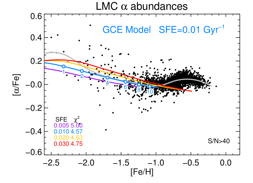
Figure 18.— The $\alpha$ abundances for the LMC with various galactic chemical evolution model sampling a range of SFE. The model $\alpha$ abundance is the mean of [Mg/Fe], [O/Fe], [Ca/Fe] and [Si/Fe]. The best-fitting model to the metal-poor stars ([Fe/H]$<$$-$1.2) has SFE=0.01 Gyr^-1. Certain times are indicated by open circles. None of these models match the flat (and rising) $\alpha$ distribution at the metal-rich end.

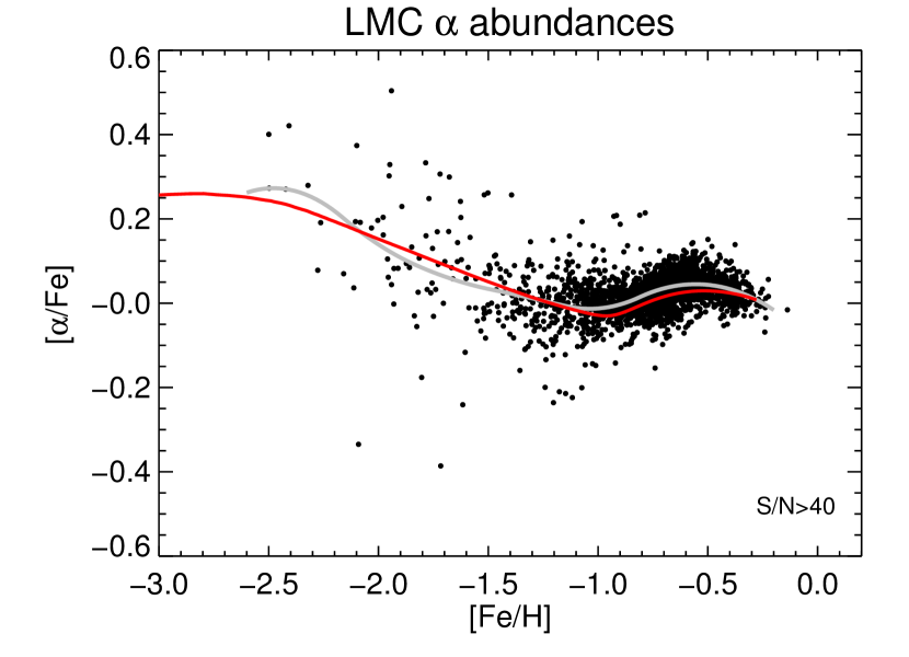
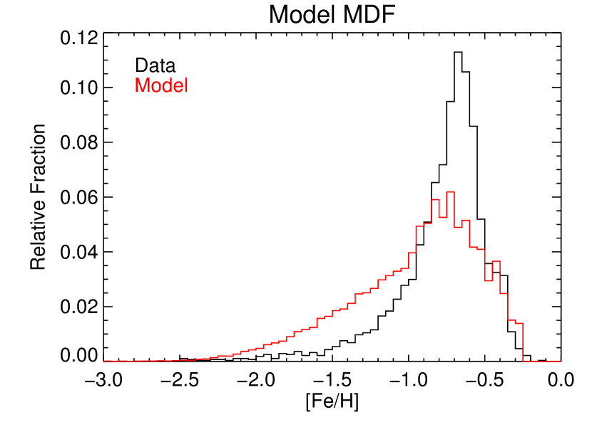
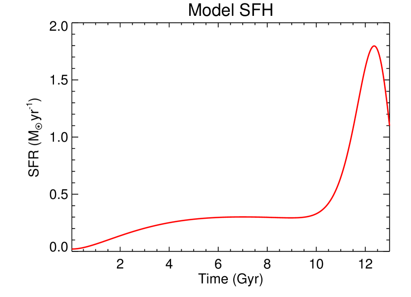
Figure 19.— Comparison of our best-fitting galactic one-zone chemical “starburst” evolution model with a recent starburst. (Top) The $\alpha$ abundances for the LMC (black dots) with a trendline (gray) and chemical evolution model (red). (Middle) The metallicity distribution function of the data (black) and model (red). The model matches the shape of the data well but is slightly too metal-poor by$-$0.15 dex. (Bottom) The star formation history of the chemical evolution model indicating the rapid increase in the star formation rate from $\sim$0.24$\times$10^-10 M${}_{\odot}~{}$yr^-1 pc^-2 for the first $\sim$10 Gyr to 2.1$\times$10^-10 M${}_{\odot}~{}$yr^-1 pc^-2 (an increase of $\sim$8.75$\times$) at the peak of the “starburst” over the last couple Gyrs.

Despite the fit to the metal-poor stars, most of these models barely enrich to [Fe/H] $\sim$ $-$1.0, and none reproduce the flat or increasing $\alpha$-element abundance pattern seen in the LMC at higher metallicities. An increasing $\alpha$-element abundance pattern at these metallicities is, however, not entirely unexpected. Bekki & Tsujimoto (2012) modeled the LMC $\alpha$-element abundance patterns using a variety of SFHs, including models where the LMC underwent a burst of SFH starting about 2 Gyr ago, which produces a bump in [Mg/Fe] ratios as a function of metallicity owing to an increased contribution of core-collapse SNe for a relatively short duration that gives way once again to a dominating Fe contribution from Type Ia SNe. While the model comparisons to the data in Bekki & Tsujimoto (2012) were not entirely conclusive that this was the best SFH model, they were consistent with producing a modest increase in [Mg/Fe] beginning at [Fe/H] $\sim$ $-$1.0 followed by a decrease in [Mg/Fe] beginning at [Fe/H] $\sim$ $-$0.5. With a larger and more precise sample, we are now able to see this predicted “bump” in the [Mg/Fe] ratios (and other $\alpha$-elements), which motivates trying to model a burst or increase in SFR to reproduce this feature following the lead of Bekki & Tsujimoto (2012).

To modify our best-fit model in flexCE to simulate a starburst in the LMC’s chemical evolution history, we alter the SFE to be time dependent, allowing for bursts of star formation that could be triggered by events such as interactions with the SMC, without requiring an infall of gas (which could also be triggered by an interaction with the SMC). We model a burst or increase in star formation by adding a Gaussian shaped increase in SFE on top of the constant SFE already in the models (see bottom panel of Figure 19). By varying the time of the burst, its duration, and its strength, we find that we can not only reach higher metallicities than constant SFE models, but can also produce the increase and subsequent decrease in [$\alpha$/Fe] seen in the abundance pattern of the LMC at metallicities [Fe/H] $\gtrsim$ $-$1.0.

Our best burst model, shown in Figure 19, uses essentially the same parameters as the best-fit model to the metal-poor end of the LMC abundance distribution given above, except with a slightly modified base SFE_i = 0.0125 Gyr^-1 that later undergoes an increase following a Gaussian form with a duration of $\sigma_{\tau}=1.5$ Gyr, peaking at $\mu_{\tau}=15.25$ Gyr, with a 35$\times$ increase in SFE (i.e., SFE_peak = 0.35 Gyr^-1). Because the peak of the SFE is outside the model run time of 13 Gyr, the actual peak SFR occurs around 12.25 Gyr, because the gas available for star formation depletes more rapidly during the starburst, and produces a factor of 6 increase in the SFR.

Altogether, this best model produces a SFH with a low and slow SFR for the majority of LMC’s history, which produces the low-metallicity end of the LMC’s chemical-abundance patterns, which is kickstarted within the past 2–3 Gyr with a recent burst of star formation producing the high-metallicity population of the LMC. Looking at the $\alpha$-element abundance pattern of our burst model, we can see that the model passes through the low-metallicity end of the LMC abundance distribution, although there is a large scatter that is likely due to a combination of higher uncertainties in metal-poor stars and their intrinsic scatter. This model also reproduces the rise and slight turnover seen in the [$\alpha$/Fe] ratio at metallicities [Fe/H] $\gtrsim-1$ that were difficult to reproduce with constant SFE models.

By binning the model in metallicity, and normalizing by the surviving population of stars at each time step, we can also compare the expected metallicity distribution function (MDF) of the chemical evolution model to the observed MDF (normalized by the number of stars in our LMC sample with S/N $>50$). In general, the shape of the model MDF is similar to the observed MDF, although it is shifted to lower metallicities by $\sim$0.15 dex. This shift could suggest that a chemical evolution model with a slightly higher base SFE may be more appropriate, although higher SFEs were slightly less preferred when fitting to only the metal-poor LMC abundance profiles.

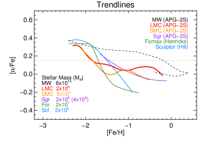
Figure 20.— (Left) A comparison of the $\alpha$-element abundance patterns of various Local Group galaxies. The MW, LMC, SMC, and Sgr trendlines come from APOGEE-2S data (using [Mg+Ca+Si/Fe]) while that for Fornax (using [Mg/Fe]) is from Hendricks et al. (2014) and that for Sculptor (using [Mg+Ca+Si/Fe]) is from (Hill et al., 2018). The [$\alpha$/Fe]=$+$0.15 line used to measure [Fe/H]_α0.15 is shown in gray. (Right) The [Fe/H] position where the $\alpha$-element abundance trendline crosses [$\alpha$/Fe]=$+$0.15 ([Fe/H]_α0.15) versus $M_{V}$ for various dwarf galaxies with bootstrap uncertainties. The APOGEE-2 abundances were used for the LMC, SMC, and Sgr, while the Kirby et al. (2010) abundances were used for the rest of the dwarf galaxies. The best linear fit to the low-luminosity galaxies is shown as a black-dashed line. The Magellanic Clouds are clearly outliers, with significantly more metal-poor $\alpha$-element abundance trendlines than expected for their absolute magnitudes or mass.

Qualitatively, this old and slow SFH with a recent burst in the past few Gyr is similar to the SFHs found by photometric studies (e.g., Meschin et al., 2014). However, the presence of stars with low $\alpha$-element abundances, even at metallicities of [Fe/H] $\sim-1.5$, and an increasing [$\alpha$/Fe] abundance pattern with decreasing metallicity seem to imply a relatively slower early SFH than found by the photometric studies, which are more limited in their metallicity discrimination. However, this discrepancy should be revisited when more metal-poor stars are included in LMC chemical evolution analyses. Regardless of the specific SFE at low metallicities, the fact that metallicities above [Fe/H] $\sim-1$ in the model are produced within the burst of star formation within the last 2–3 Gyr of the model, implies that the majority of stars we have observed in the LMC using APOGEE have been formed within the past 2–3 Gyr. While an age analysis is beyond the scope of this paper, we do find that the most metal-rich stars in our sample are likely blue-loop stars, as shown in Figure 15. If so, this would imply that their masses are $\sim$ 3 $M_{\odot}$, which supports that the metal-rich stars are rather young.

7. Discussion

Compared to many other MW dwarf galaxies, the $\alpha$-element abundance trendlines of the MCs (as measured by APOGEE) are more metal poor. Trendlines using B-splines are shown in the left panel of Figure 20, where we compare the [$\alpha$/Fe]–[Fe/H] trendlines of other galaxies in the literature to our MC trendlines. We find that the MCs $\alpha$-element abundance trendlines (and their knees) are more metal poor than Fornax, Sculptor, and Sgr, even though the MCs are a factor of $\sim$100–1000 more massive in stellar mass.

The MW dwarf galaxies show a range in $\alpha$-knees, as shown by the compilation in Hendricks et al. (2014). The $\alpha$-knee is sensitive to the early SFR and Hendricks et al. suggest that there is a relationship between the $\alpha$-knee of the galaxy and its absolute magnitude (and possibly stellar mass). However, the $\alpha$-knee is challenging to measure because it requires having reliable $\alpha$-element abundances for a statistically significant number of metal-poor stars, and because some dwarf galaxies only show a linear increase at low metallicity without any clear sign of reaching a plateau. Therefore, to reliably compare the $\alpha$-element abundances of the dwarf galaxies, we establish a new metric that measures the position of the steeply falling portion of the $\alpha$-element abundances at low metallicity or “$\alpha$-shin”. We define [Fe/H]_α0.15 as the metallicity where the $\alpha$-element trendline crosses [$\alpha$/Fe]=$+$0.15. The right panel of Figure 20 shows [Fe/H]_α0.15 versus $M_{\rm V}$ for eleven MW dwarf galaxies using APOGEE-2 abundances for LMC, SMC, and Sgr, while the Kirby et al. (2010) abundances for the rest of the dwarf galaxies. For the APOGEE data the trendlines were fit using a B-spline to the [$\alpha$/Fe] abundances, while for the Kirby et al. data trendlines were fit for each $\alpha$-element separately and then averaged. Uncertainties in [Fe/H]_α0.15 were determined using a bootstrap technique using 100 mocks. For the lower luminosity dwarfs ($M_{\rm V}$ $>$ $-$14) an anti-correlation is apparent, similar to the anti-correlation presented by Hendricks et al. (2014). The best-fit linear trend is indicated by the dashed line, and has a Pearson correlation coefficient of $-$0.705, which indicates a strong anti-correlation. The MCs clearly fall off this correlation, and their $\alpha$-element abundance trends are significantly more metal-poor than expected for their higher luminosities.

So why are the MCs so “lazy” early-on in their evolution? One major difference between the MCs and the rest of the dwarf galaxies in Figure 20 is the environment in which they formed and evolved. The MCs are likely falling into the MW gravitational potential well for the first time (e.g., Besla et al., 2007, 2012), and have presumably been forming stars in isolation for roughly 10 Gyr. If the other galaxies with more metal-rich $\alpha$-element knees fell into the MW potential well early on in their formation, it is possible they have artificially high SFE from tidal interactions with the MW, and/or experienced enhanced star formation during ram pressure stripping. Gallart et al. (2015) derived precise star formation histories from deep $HST$ imaging of LG dwarf galaxies, and found that the early star formation rate of the dwarf galaxies depended on the density of their environment, with “slow” dwarfs forming in relatively isolated regions. In this context, the slow early star formation of the MCs adds even more support to the hypothesis that the MCs fell into the MW potential only recently. If the low SFE of the MCs is an environmental effect, then we would expect that Magellanic satellites, such as the ones recently discovered (Hor1, Car2, Car3, and Hyi1; Bechtol et al., 2015; Torrealba et al., 2018; Li et al., 2018; Koposov et al., 2018; Kallivayalil et al., 2018), should also have low SFE and metal-poor $\alpha$-element abundance trendlines. Future abundance studies will help resolve whether this is indeed the case.

However, as discussed in §6.3, it is not possible for the LMC to enrich its gas to the level seen today with the SFE responsible for the metal-poor knee. We argue that the observed bump in [$\alpha$/Fe] is indicative of a large starburst some 2–3 Gyr ago (e.g., Harris & Zaritsky, 2009), which is then responsible for enriching the galaxy from [Fe/H] = $-$1.0 to [Fe/H]$\approx$ $-$0.2. Without the recent starburst, likely created by a close interaction with the SMC (e.g., Harris & Zaritsky, 2009; Besla et al., 2012), the LMC chemical-abundance patterns and MDF would be substantially different than we see today. While we do not observe increasing [$\alpha$/Fe] with increasing [Fe/H] beyond the knee in any of the other galaxies, we do observe a flat [$\alpha$/Fe] with increasing [Fe/H] for the SMC, Sgr, and Fornax (from Hendricks et al., 2014). A flat [$\alpha$/Fe] abundance pattern can be produced with a weak starburst (or starbursts), that enrich the ISM with metals and prevent the further dilution of [$\alpha$/Fe] by Type Ia SNe, but are too weak to produce substantial [$\alpha$/Fe] enhancement.

Hendricks et al. (2014) found that they were able to recreate the Fornax $\alpha$-element abundance patterns by using a chemical evolution model with three distinct starbursts that varied in SFE, but were all more efficient than the initial starburst. There is a thread of work in the literature that finds evidence for a recent merger in Fornax from spatial and kinematical substructure (e.g., Coleman et al., 2004; Yozin & Bekki, 2012; del Pino et al., 2015), which could be responsible for causing these starbursts. In the case of the MCs, the starbursts were likely triggered by a close interaction between the MCs some 2–3 Gyr ago. Evidence for such an interaction is motivated by cotemporal starbursts, dynamical simulations, and studies of Magellanic stellar substructures (e.g., Harris & Zaritsky, 2009; Besla et al., 2012, 2016; Choi et al., 2018a, b; Belokurov et al., 2018).

8. Summary

We have obtained 3800 high-resolution $H$-band spectra of stars in the Large and Small Magellanic Clouds (MCs) using the new Southern APOGEE instrument on the du Pont telescope at Las Campanas Observatory. This sizable stellar sample covers a large radial and azimuthal range of the MCs. The stars cover a large metallicity range ($-$2.5$<$[Fe/H]$<$ $-$0.2), and the $\alpha$-element distributions reveal important insights into the chemical evolution of the MCs. The main conclusions from our analysis of our red giant branch sample are:

1. The [$\alpha$/Fe]–[Fe/H] distributions of the MCs are quite flat over a large range in metallicity, $-$1.2$<$[Fe/H]$<$ $-$0.2.

2. There is an increase of $\sim$0.1 dex in [$\alpha$/Fe] from [Fe/H] = $-$1.0 to [Fe/H] = $-$0.5, with a small decrease for the youngest and most metal-rich LMC stars at [Fe/H] $>$ $-$0.5. This behavior can be explained by a recent increase in sta-formation activity in the MCs. Our one-zone chemical evolution models are able to reproduce this $\alpha$-element abundance “bump” with such a recent starburst.

3. We constrain the position of the “$\alpha$-knee” to be at [Fe/H]$\lesssim$ $-$2.2 for both the LMC and the SMC. We define a new metric, [Fe/H]_α0.15, the metallicity where the $\alpha$-element trendline crosses [$\alpha$/Fe]=$+$0.15, to reliably inter-compare $\alpha$-element abundance trends between dwarf galaxies. Chemical evolution models fitted to the abundances of the metal-poor stars in the LMC find a low SFE of $\approx$0.01 Gyr^-1 with a gas consumption timescale of $\approx$100 Gyr.

4. The LMC and SMC $\alpha$-element abundance trendlines are more metal poor than those for less massive MW satellites such as Fornax, Sculptor, or Sagittarius and the MCs are large outliers in [Fe/H]_α0.15–$M_{\rm V}$ for MW satellites. This counter-intuitive result suggests that the MCs formed in a lower-density environment, which is consistent with the paradigm that the MCs fell into the MW potential only recently.

Table 1APOGEE Magellanic Clouds Fields

Name	RA	DEC	$L_{\rm MS}$	$B_{\rm MS}$	$R$	PA	NVisits	NVisits	NMC	NMC,RGB	NMC,RGB	NMC,RGB,S/N>40
	(J2000)	(J2000)	(deg)	(deg)	(deg)	(deg)	Planned		Targets	Targets	Members	Members
SMC1	00:20:16.9	$-$77:13:21.3	$-$11.96	$-$14.98	4.9	202	12	11	332	82	48	29
47Tuc	00:24:39.5	$-$72:09:26.8	$-$16.91	$-$13.34	2.2	284	12	10	411	98	87	86
SMC2	00:41:58.6	$-$67:45:25.4	$-$20.66	$-$10.50	5.2	349	12	8	365	132	109	77
SMC3	00:45:00.1	$-$73:13:45.1	$-$15.37	$-$12.26	0.7	234	12	8	442	289	273	259
NGC362	00:57:32.9	$-$71:05:40.3	$-$16.99	$-$10.54	1.8	13	12	10	309	146	139	138
SMC4	01:07:56.2	$-$75:35:35.4	$-$12.52	$-$11.80	3.0	161	12	8	275	188	180	175
SMC5	01:20:41.2	$-$73:04:48.0	$-$14.37	$-$9.86	2.1	100	12	6	307	174	169	158
SMC6	01:38:29.9	$-$71:09:11.1	$-$15.30	$-$7.69	3.9	70	12	6	279	189	182	142
SMC7	02:07:23.7	$-$73:24:29.7	$-$12.15	$-$7.30	5.4	105	12	9	351	88	55	40
LMC1	04:10:18.1	$-$71:56:58.5	$-$5.54	$-$0.93	6.6	243	9	4	323	173	147	85
LMC2	04:10:22.6	$-$68:26:59.8	$-$6.77	2.34	7.0	273	9	6	329	138	108	71
LMC3	04:46:05.2	$-$75:19:58.6	$-$2.17	$-$3.46	6.3	205	9	10	282	190	186	184
LMC4	04:52:44.1	$-$68:48:13.5	$-$2.96	3.04	3.3	285	9	4	400	263	255	252
LMC5	04:55:38.7	$-$71:18:17.7	$-$2.27	0.62	3.0	238	9	7	366	239	234	202
LMC6	05:11:02.4	$-$65:40:47.7	$-$1.66	6.39	4.5	338	9	6	359	206	202	200
LMC7	05:14:06.1	$-$62:33:57.9	$-$1.65	9.52	7.4	348	9	3	278	177	175	171
LMC8	05:19:43.7	$-$72:49:04.1	$-$0.25	$-$0.65	3.0	191	9	12	349	228	225	225
LMC9	05:22:23.8	$-$69:42:36.7	$-$0.24	2.47	0.5	289	9	5	251	152	142	129
LMC10	05:31:22.4	$-$76:10:04.7	0.69	$-$3.96	6.3	178	9	6	275	176	168	162
30Dor	05:36:13.6	$-$69:07:40.0	0.96	3.09	1.1	47	1	4	173	53	41	4
LMC11	05:41:31.0	$-$63:34:43.1	1.53	8.63	6.4	14	9	2	264	186	182	179
LMC12	05:44:47.3	$-$60:23:34.1	2.00	11.81	9.6	13	9	2	223	128	90	36
LMC13	05:46:05.6	$-$67:42:34.9	1.89	4.49	2.7	40	9	2	258	177	172	168
LMC14	05:53:21.1	$-$70:58:13.7	2.36	1.20	2.4	120	9	4	262	157	154	152
LMC15	06:08:30.6	$-$63:35:53.7	4.55	8.39	7.4	38	9	0	260	215	0	0
LMC16	06:32:17.2	$-$75:11:03.3	4.54	$-$3.37	7.2	145	9	6	252	149	122	97
LMC17	06:32:47.1	$-$70:18:34.9	5.68	1.37	5.6	102	9	10	269	178	172	170

References

- Abolfathi et al. (2018) Abolfathi, B., Aguado, D. S., Aguilar, G., et al. 2018, ApJS, 235, 42
- Alvarez & Plez (1998) Alvarez, R., & Plez, B. 1998, A&A, 330, 1109
- Andrews et al. (2017) Andrews, B. H., Weinberg, D. H., Schönrich, R., & Johnson, J. A. 2017, ApJ, 835, 224
- Bechtol et al. (2015) Bechtol, K., Drlica-Wagner, A., Balbinot, E., et al. 2015, ApJ, 807, 50
- Bekki & Tsujimoto (2012) Bekki, K., & Tsujimoto, T. 2012, ApJ, 761, 180
- Belokurov et al. (2018) Belokurov, V., Erkal, D., Evans, N. W., Koposov, S. E., & Deason, A. J. 2018, MNRAS, 478, 611
- Belokurov & Erkal (2019) Belokurov, V. A., & Erkal, D. 2019, MNRAS, 482, L9
- Bermejo-Climent et al. (2018) Bermejo-Climent, J. R., Battaglia, G., Gallart, C., et al. 2018, MNRAS, 479, 1514
- Besla et al. (2007) Besla, G., Kallivayalil, N., Hernquist, L., et al. 2007, ApJ, 668, 949
- Besla et al. (2012) —. 2012, MNRAS, 421, 2109
- Besla et al. (2016) Besla, G., Martínez-Delgado, D., van der Marel, R. P., et al. 2016, ApJ, 825, 20
- Blanton et al. (2017) Blanton, M. R., Bershady, M. A., Abolfathi, B., et al. 2017, AJ, 154, 28
- Bonanos et al. (2009) Bonanos, A. Z., Massa, D. L., Sewilo, M., et al. 2009, AJ, 138, 1003
- Brown et al. (2018) Brown, A. G. A., Vallenari, A., Prusti, T., & de Bruijne, J. H. J. 2018, Astronomy & Astrophysics, doi:10.1051/0004-6361/201833051
- Buder et al. (2018) Buder, S., Asplund, M., Duong, L., et al. 2018, MNRAS, 478, 4513
- Calura et al. (2009) Calura, F., Pipino, A., Chiappini, C., Matteucci, F., & Maiolino, R. 2009, A&A, 504, 373
- Carlin et al. (2018) Carlin, J. L., Sheffield, A. A., Cunha, K., & Smith, V. V. 2018, ApJ, 859, L10
- Carretta et al. (2009a) Carretta, E., Bragaglia, A., Gratton, R., D’Orazi, V., & Lucatello, S. 2009a, A&A, 508, 695
- Carretta et al. (2009b) Carretta, E., Bragaglia, A., Gratton, R., & Lucatello, S. 2009b, A&A, 505, 139
- Chieffi & Limongi (2004) Chieffi, A., & Limongi, M. 2004, ApJ, 608, 405
- Choi et al. (2018a) Choi, Y., Nidever, D. L., Olsen, K., et al. 2018a, ApJ, 866, 90
- Choi et al. (2018b) —. 2018b, ApJ, 869, 125
- Coleman et al. (2004) Coleman, M., Da Costa, G. S., Bland-Hawthorn, J., et al. 2004, AJ, 127, 832
- Dark Energy Survey Collaboration et al. (2016) Dark Energy Survey Collaboration, Abbott, T., Abdalla, F. B., et al. 2016, MNRAS, 460, 1270
- de Boer et al. (2014) de Boer, T. J. L., Belokurov, V., Beers, T. C., & Lee, Y. S. 2014, MNRAS, 443, 658
- Dekel & Silk (1986) Dekel, A., & Silk, J. 1986, ApJ, 303, 39
- del Pino et al. (2015) del Pino, A., Aparicio, A., & Hidalgo, S. L. 2015, MNRAS, 454, 3996
- Dell’Agli et al. (2015a) Dell’Agli, F., García-Hernández, D. A., Ventura, P., et al. 2015a, MNRAS, 454, 4235
- Dell’Agli et al. (2015b) Dell’Agli, F., Ventura, P., Schneider, R., et al. 2015b, MNRAS, 447, 2992
- Dolphin (2002) Dolphin, A. E. 2002, MNRAS, 332, 91
- Drlica-Wagner et al. (2015) Drlica-Wagner, A., Bechtol, K., Rykoff, E. S., et al. 2015, ApJ, 813, 109
- Eisenstein et al. (2011) Eisenstein, D. J., Weinberg, D. H., Agol, E., et al. 2011, AJ, 142, 72
- Fillingham et al. (2018) Fillingham, S. P., Cooper, M. C., Boylan-Kolchin, M., et al. 2018, MNRAS, 477, 4491
- Gallart et al. (2015) Gallart, C., Monelli, M., Mayer, L., et al. 2015, ApJ, 811, L18
- García Pérez et al. (2016) García Pérez, A. E., Allende Prieto, C., Holtzman, J. A., et al. 2016, AJ, 151, 144
- Grcevich & Putman (2009) Grcevich, J., & Putman, M. E. 2009, ApJ, 696, 385
- Gunn et al. (2006) Gunn, J. E., Siegmund, W. A., Mannery, E. J., et al. 2006, AJ, 131, 2332
- Gustafsson et al. (2008) Gustafsson, B., Edvardsson, B., Eriksson, K., et al. 2008, A&A, 486, 951
- Harris & Zaritsky (2009) Harris, J., & Zaritsky, D. 2009, AJ, 138, 1243
- Hasselquist et al. (2017) Hasselquist, S., Shetrone, M., Smith, V., et al. 2017, ApJ, 845, 162
- Hawkins et al. (2016) Hawkins, K., Masseron, T., Jofré, P., et al. 2016, A&A, 594, A43
- Hendricks et al. (2014) Hendricks, B., Koch, A., Lanfranchi, G. A., et al. 2014, ApJ, 785, 102
- Hill et al. (2018) Hill, V., Skúladóttir, Á., Tolstoy, E., et al. 2018, arXiv e-prints, arXiv:1812.01486
- Holtzman et al. (2015) Holtzman, J. A., Shetrone, M., Johnson, J. A., et al. 2015, AJ, 150, 148
- Hopkins et al. (2013) Hopkins, P. F., Kereš, D., Murray, N., et al. 2013, MNRAS, 433, 78
- Iwamoto et al. (1999) Iwamoto, K., Brachwitz, F., Nomoto, K., et al. 1999, ApJS, 125, 439
- Jönsson et al. (2018) Jönsson, H., Allende Prieto, C., Holtzman, J. A., et al. 2018, AJ, 156, 126
- Kallivayalil et al. (2018) Kallivayalil, N., Sales, L. V., Zivick, P., et al. 2018, ApJ, 867, 19
- Kamath et al. (2014) Kamath, D., Wood, P. R., & Van Winckel, H. 2014, MNRAS, 439, 2211
- Kamath et al. (2015) —. 2015, MNRAS, 454, 1468
- Karakas (2010) Karakas, A. I. 2010, MNRAS, 403, 1413
- Kirby et al. (2013) Kirby, E. N., Cohen, J. G., Guhathakurta, P., et al. 2013, ApJ, 779, 102
- Kirby et al. (2010) Kirby, E. N., Guhathakurta, P., Simon, J. D., et al. 2010, ApJS, 191, 352
- Koposov et al. (2018) Koposov, S. E., Walker, M. G., Belokurov, V., et al. 2018, MNRAS, 479, 5343
- Köppen et al. (2007) Köppen, J., Weidner, C., & Kroupa, P. 2007, MNRAS, 375, 673
- Kroupa (2001) Kroupa, P. 2001, MNRAS, 322, 231
- Lapenna et al. (2012) Lapenna, E., Mucciarelli, A., Origlia, L., & Ferraro, F. R. 2012, ApJ, 761, 33
- Li et al. (2018) Li, T. S., Simon, J. D., Pace, A. B., et al. 2018, ApJ, 857, 145
- Limongi & Chieffi (2006) Limongi, M., & Chieffi, A. 2006, ApJ, 647, 483
- Majewski et al. (2009) Majewski, S. R., Nidever, D. L., Muñoz, R. R., et al. 2009, in IAU Symposium, Vol. 256, The Magellanic System: Stars, Gas, and Galaxies, ed. J. T. Van Loon & J. M. Oliveira, 51–56
- Majewski et al. (2000) Majewski, S. R., Patterson, R. J., Dinescu, D. I., et al. 2000, in Liege International Astrophysical Colloquia, Vol. 35, Liege International Astrophysical Colloquia, ed. A. Noels, P. Magain, D. Caro, E. Jehin, G. Parmentier, & A. A. Thoul, 619
- Majewski et al. (2017) Majewski, S. R., Schiavon, R. P., Frinchaboy, P. M., et al. 2017, AJ, 154, 94
- Masseron et al. (2016) Masseron, T., Merle, T., & Hawkins, K. 2016, BACCHUS: Brussels Automatic Code for Characterizing High accUracy Spectra, Astrophysics Source Code Library, ascl:1605.004
- Masseron et al. (2019) Masseron, T., García-Hernández, D. A., Mészáros, S., et al. 2019, A&A, 622, A191
- Mateo (1998) Mateo, M. L. 1998, ARA&A, 36, 435
- Matteucci (1994) Matteucci, F. 1994, A&A, 288, 57
- McConnachie (2012) McConnachie, A. W. 2012, AJ, 144, 4
- McWilliam (1997) McWilliam, A. 1997, ARA&A, 35, 503
- Meschin et al. (2014) Meschin, I., Gallart, C., Aparicio, A., et al. 2014, MNRAS, 438, 1067
- Mészáros et al. (2013) Mészáros, S., Holtzman, J., García Pérez, A. E., et al. 2013, AJ, 146, 133
- Muñoz et al. (2006) Muñoz, R. R., Majewski, S. R., Zaggia, S., et al. 2006, ApJ, 649, 201
- Mucciarelli (2014) Mucciarelli, A. 2014, Astronomische Nachrichten, 335, 79
- Neugent et al. (2012) Neugent, K. F., Massey, P., Skiff, B., & Meynet, G. 2012, ApJ, 749, 177
- Nidever et al. (2015) Nidever, D. L., Holtzman, J. A., Allende Prieto, C., et al. 2015, AJ, 150, 173
- Nidever et al. (2017) Nidever, D. L., Olsen, K., Walker, A. R., et al. 2017, AJ, 154, 199
- Nidever et al. (2018) Nidever, D. L., Olsen, K., Choi, Y., et al. 2018, arXiv e-prints, arXiv:1805.02671
- Nikolaev & Weinberg (2000) Nikolaev, S., & Weinberg, M. D. 2000, ApJ, 542, 804
- Olsen et al. (2011) Olsen, K. A. G., Zaritsky, D., Blum, R. D., Boyer, M. L., & Gordon, K. D. 2011, ApJ, 737, 29
- Pearson et al. (2016) Pearson, S., Besla, G., Putman, M. E., et al. 2016, MNRAS, 459, 1827
- Plez (2012) Plez, B. 2012, Turbospectrum: Code for spectral synthesis, Astrophysics Source Code Library, ascl:1205.004
- Pompéia et al. (2008) Pompéia, L., Hill, V., Spite, M., et al. 2008, A&A, 480, 379
- Rubele et al. (2012) Rubele, S., Kerber, L., Girardi, L., et al. 2012, A&A, 537, A106
- Sakari et al. (2017) Sakari, C. M., McWilliam, A., & Wallerstein, G. 2017, MNRAS, 467, 1112
- Searle & Zinn (1978) Searle, L., & Zinn, R. 1978, ApJ, 225, 357
- Simha et al. (2014) Simha, V., Weinberg, D. H., Conroy, C., et al. 2014, arXiv e-prints, arXiv:1404.0402
- Skrutskie et al. (2006) Skrutskie, M. F., Cutri, R. M., Stiening, R., et al. 2006, AJ, 131, 1163
- Smecker-Hane et al. (2002) Smecker-Hane, T. A., Cole, A. A., Gallagher, III, J. S., & Stetson, P. B. 2002, ApJ, 566, 239
- Smith et al. (2000) Smith, V. V., Suntzeff, N. B., Cunha, K., et al. 2000, AJ, 119, 1239
- Tinsley (1979) Tinsley, B. M. 1979, ApJ, 229, 1046
- Torrealba et al. (2018) Torrealba, G., Belokurov, V., Koposov, S. E., et al. 2018, MNRAS, 475, 5085
- van den Bergh (1999) van den Bergh, S. 1999, A&A Rev., 9, 273
- Van der Swaelmen et al. (2013) Van der Swaelmen, M., Hill, V., Primas, F., & Cole, A. A. 2013, A&A, 560, A44
- Weisz et al. (2013) Weisz, D. R., Dolphin, A. E., Skillman, E. D., et al. 2013, MNRAS, 431, 364
- Weisz et al. (2014) —. 2014, ApJ, 789, 147
- Wetzel et al. (2015) Wetzel, A. R., Tollerud, E. J., & Weisz, D. R. 2015, ApJ, 808, L27
- Willman (2010) Willman, B. 2010, Advances in Astronomy, 2010, 285454
- Wilson et al. (2019) Wilson, J. C., Hearty, F. R., & Skrutskie, M. F. 2019, PASA, 999, 999
- Yozin & Bekki (2012) Yozin, C., & Bekki, K. 2012, ApJ, 756, L18
- Zamora et al. (2015) Zamora, O., García-Hernández, D. A., Allende Prieto, C., et al. 2015, AJ, 149, 181
- Zasowski et al. (2013) Zasowski, G., Johnson, J. A., Frinchaboy, P. M., et al. 2013, AJ, 146, 81
- Zasowski et al. (2017) Zasowski, G., Cohen, R. E., Chojnowski, S. D., et al. 2017, AJ, 154, 198
- Zasowski et al. (2019) Zasowski, G., Schultheis, M., Hasselquist, S., et al. 2019, ApJ, 870, 138