monthyeardate\monthname[\THEMONTH] \THEDAY, \THEYEAR
Decision Directed Channel Estimation Based on Deep Neural Network -step Predictor for MIMO Communications in 5G
††thanks: M. Mehrabi, M. Mohammadkarimi, M. Ardakani, and Y. Jing are with the
Faculty of Electrical and Computer Engineering, University of Alberta, Edmonton, AB, Canada.
(e-mail: {mehrtash, mostafa.mohammadkarimi, ardakani, yindi}@ualberta.ca).
Abstract
We consider the use of deep neural network (DNN) to develop a decision-directed (DD)- channel estimation (CE) algorithm for multiple-input multiple-output (MIMO)-space-time block coded systems in highly dynamic vehicular environments. We propose the use of DNN for -step channel prediction for space-time block code (STBC)s, and show that deep learning (DL)-based DD-CE can removes the need for Doppler spread estimation in fast time-varying quasi stationary channels, where the Doppler spread varies from one packet to another. Doppler spread estimation in this kind of vehicular channels is remarkably challenging and requires a large number of pilots and preambles, leading to lower power and spectral efficiency. We train two DNNs which learn real and imaginary parts of the MIMO fading channels over a wide range of Doppler spreads. We demonstrate that by those DNNs, DD-CE can be realized with only rough priori knowledge about Doppler spread range. For the proposed DD-CE algorithm, we also analytically derive the maximum likelihood (ML) decoding algorithm for STBC transmission. The proposed DL-based DD-CE is a promising solution for reliable communication over the vehicular MIMO fading channels without accurate mathematical models. This is because DNN can intelligently learn the statistics of the fading channels. Our simulation results show that the proposed DL-based DD-CE algorithm exhibits lower propagation error compared to existing DD-CE algorithms while the latters require perfect knowledge of the Doppler rate.
Index Terms:
MIMO communication, channel estimation, deep learning, decision directed, mmWave communications.I Introduction
I-A Motivation
Wireless data traffic has been growing rapidly and according to a Cisco report [1], global wireless data traffic will increase sevenfold between 2016 and 2021, reaching 49.0 exabytes per month by 2021. This wireless data explosion is expected to accelerate over the next decade by increasing the popularity of smartphones, continual use of wireless video streaming services, and the rise of the Internet-of-Things (IoT) [2, 3].
In order to address this high volume of data traffic demand, one promising solution is to enable the use of higher frequency spectrum, e.g., millimeter wave (mmWave) [3, 4]. Currently, the fifth-generation (5G) wireless communications is being developed based on utilizing mmWave frequencies (30-300 GHz) to provide a notable spectrum and high data rates on the order of Gbps [4]. Utilizing mmWave in MIMO communication systems is one of the candidate technologies for 5G wireless standardization [5] which can further improve the system capacity. It also benefits from spatial diversity against small-scale fading, higher data rates, and the ability to cancel interference [6, 7, 8]. In addition to spatial diversity due to multiple transmit and receive antennas, time diversity can also be achieved through STBC. STBC is an advanced transmission technique used in multiple antenna systems to transmit multiple replicas of information symbols to exploit the various received versions of the transmitted symbols to improve the reliability of transmission.
In the design of a MIMO wireless communication system in 5G, there are two main challenges that affect the performance, namely channel modeling and CE. Due to the complex propagation characteristics of highly dynamic channels, channel modeling is an extremely challenging task [9]. Furthermore, in highly dynamic environments, the channel impulse response varies quickly, and thus, the channel statistics remain constant only for a very short period of time. Consequently, the high channel variations limits the channel modeling and reduces the performance of existing channel estimators [10]. These constraints on CE in highly dynamic environments are even more crucial for STBC transmission where more channels must be estimated for each block transmission and its associated decoding process is considerably affected by the accuracy of CE method.
For MIMO systems, CE schemes have been mostly based on pilot-assisted approaches, assuming a quasi-static fading model that allows the channel to be constant for a block of symbols and change independently to a new realization. This is not applicable for environments such as fast time-varying channels where the coherence time is considerably short. Currently, DD-CE methods have been suggested to be employed in time-varying channels and it has been widely used in vehicular communication systems based on IEEE 802.11p technology [11]. In DD-CE, first a block of training symbols is sent to estimate the channel state information (CSI). Then, data transmissions are conducted, where the subsequent CSI corresponding to the data symbols are predicted by treating the detected symbols as training data and re-estimating the channel iteratively [12, 13]. The core part of the DD-CE is channel prediction. Existing channel predictors are highly depended on channel statistics which is severely affected by the estimation of Doppler spread of the channel. However, in highly dynamic vehicular environments, Doppler spread estimation is challenging.
Recently, DL has been widely investigated in the signal processing and communications problems to improve the performance of some certain parts of conventional communication systems, such as decoding, estimation, and more [14, 15, 16, 17, 18, 19, 20, 21]. In particular, DL-based CE methods have been studied in literature such as the recent work in [14]. A DNN is a universal function approximator with superior logarithmic learning ability and convenient optimization capability, and thus can be used for the problems without any accurate mathematical model [22]. Currently, most of the existing algorithms in communications rely on precise mathematical models. However, in practice tractable mathematical models cannot reflect many imperfections and nonlinearities, and can only work as rough approximations when these issues are non-negligible. DL can fix this drawback in communication and information theory and offer algorithms without mathematically tractable models [18].
Motivated by the limitations of existing channel predictors and the strength of DNN in learning and prediction, a DL-based DD-CE for MIMO STBC is proposed in this paper, where the MIMO channel coefficients are predicted by two trained DNNs. While existing channel predictors require the exact value of Doppler spread and an accurate mathematical model for Doppler spectrum, our proposed algorithm does not require Doppler spread estimation and provides a more reliable packet transmission in highly dynamic vehicular environments. Moreover, we derive the maximum likelihood (ML) STBC decoding for any STBC design in fast time-varying channels, where channels vary during each STBC transmission. In the proposed scheme, first we predict the corresponding channels for each block transmission and then perform signal detection with the channel prediction.
I-B Related Work
1) DD-CE channel predictors: The optimal Weiner filter, finite length Wiener filter, and weighted recursive least squares (LS), such as Kalman filter (KF), are the most popular predictors employed in DD-CE [23, 24] where all of them rely on exact Doppler spread estimation. Furthermore, inaccurate Doppler spread estimation results in significant error propagation in suboptimal channel predictors like KF, especially at high Doppler spreads and when the transmitted packets are large. In addition, the sensitivity of current channel predictors to the accuracy of the channel model is too high to tolerate any modeling errors. However, finding an explicit mathematical model to describe the channel propagation characteristics in highly dynamic environments is a challenging task and thus modeling error is inevitable.
2) CE for STBC transmission: Wireless communication systems usually rely on some form of diversity at the transmit side and/or the receiver side. STBC transmission is one of the most common solutions for achieving diversity. Alamouti introduced a well-known transmission technique for systems with two transmit antennas in [25]. By generalizing Alamouti’s idea, Tarokh et al. proposed STBC for other numbers of transmit/receive antennas [26]. The problem of CE when STBC is used for transmission has been investigated in many studies [27, 28, 29]. In the current studies, whenever STBC is used in a time-varying channel, two approaches were employed. One of them is considering a coherent channel for block transmission and the other one is channel modeling with a rough approximation such as first order autoregressive model. In [25, 29], the authors assumed that the channel is coherent for each block transmission and using this assumption, they proposed a coherent detection algorithm. However, in the fast time-varying channel where the channel statistics change rapidly, all the mentioned assumptions lead to a degraded signal detection. A KF-based CE method was used in [27, 28, 30] and it was assumed that for a block transmission the fading channel is changed based on first order Gauss-Markov process. Then after determining the channels for each block transmission, they developed a detection algorithm. Furthermore, the proposed detection algorithms are only valid for Alamouti’s scheme and for longer STBC block transmission the assumptions are not applicable [28, 29, 27].
I-C Contribution
The main contributions of this papers are as follows:
-
•
We propose a DL-based -step channel predictor;
-
•
A new DD-CE algorithm based on the proposed predictor is proposed for MIMO-STBC systems. The proposed algorithm exhibits the following advantages:
-
–
It removes the need for Doppler spread estimation;
-
–
It exhibits lower error propagation compared to existing algorithm;
-
–
It can be applied to MIMO fading channels without concrete mathematical models;
-
–
It has a lower computational complexity compared to existing DD-CE algorithms;
-
–
It is applicable to even large packets;
-
–
-
•
The joint ML decoding algorithm for general STBCs in time-varying fading channels is derived;
-
•
The proposed scheme has better performance than existing algorithms.
-
•
We derive the optimal DD-CE for general STBCs using Wiener predictor.
I-D Organization
The outline of this paper is as follows. In Section II, we briefly review DL. Section III presents the system model. Section IV introduces DD-CE method for MIMO wireless communications. Section V describes the proposed DL-based DD-CE algorithm along with our proposed ML decoding algorithm for STBC design . The complexity analysis of our proposed algorithm is presented in Section VI. Simulation results are provided in Section VII, and finally we conclude the paper in Section VIII.
I-E Notation
Throughout this paper, represents the complex conjugate. The real and imaginary parts of a complex number are denoted by and , respectively. Matrix transpose and Hermitian operators are shown by and , respectively. Moreover, the inverse of matrix is represented by and the symbol denotes the identity matrix of size . The column vector of size and all ones is denoted by . The operator returns a square diagonal matrix with the elements of vector on the main diagonal. Assuming and are some matrices with whether equal or different sizes, operator returns the following matrix
| (1) |
Furthermore, shows the absolute value, is the statistical expectation, denotes an estimated value for vector , and the Frobenius norm of vector is showed by . The constellation and -dimensional complex spaces are denoted by and , respectively. For the sake of simplicity, the element-wise notation of Matlab is used, where denotes all rows and columns of matrix , and the notation shows the -th until -th entries of vector . Note that in the sequel, and represents -th matrix and -th vector, respectively. Finally, the circularly symmetric complex Gaussian distribution with mean vector and covariance matrix is denoted by .
II Deep Learning
Deep learning is an approach to artificial intelligence and more specifically, it is a type of machine learning technique that enables computer systems to learn complicated concepts without any need for exact mathematical operators. As a result, computer systems can learn from a series of experiences to find a solution by a hierarchy of concepts where each concept is defined by simpler concepts. These concepts on top of each other, generate a deep graph to show the mapping between input and output and because of the depth of this graph this approach to artificial intelligence is called deep learning [22].
One of the quintessential DL models are deep feedforward networks, also called deep neural networks, where by training a vector of learning parameters , some function is approximated as
| (2) |
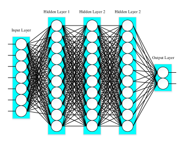
where the input vector is mapped to the output vector . The DNN breaks this complicated mapping into a series of simple ones, each defined by a distinct layer of DNN. A DNN is built by a sequence of visible and hidden layers. At visible layers, we are able to observe the variables. The input and output layers of a DNN are both visible layers. At hidden layers, the variables are not accessible and their values are changed based on the feature extraction. Fig. 1 shows a DNN with three hidden layers. For example, in a DNN with hidden layers, we can represent function in (2) by functions as
| (3) |
Each function is defined as
| (4) |
where is the output of the previous layer, denotes the set of learning parameters, and ( and ) represent weights and biases, respectively and is the activation function of the -th layer. By training the DNN with a training set and a known desired output, the weights and biases can be learned [22].
III System Model
We consider a MIMO system in a time-varying flat fading channel, where the transmitter and receiver are equipped with and antennas. The space-time encoder at the transmitter takes a block of information symbols as input and maps it into a STBC matrix as
| (5) |
where is an arbitrary constellation and , and are functions of the information vector . The columns of are generated in successive time intervals each of duration , while each of the entries in a given column is forwarded to one of the transmit antennas. At the -th transmit antenna, is first pulse shaped and then transmitted during the -th time interval. The transmitted waveforms from transmit antennas are sent simultaneously.
| (14) |
If and , independent information symbols are transmitted over each transmit antenna at each time interval, one word. This transmission scheme is referred to as the simplest case of spatial multiplexing without any need for precoding and maps a block of information symbols to the transmit antennas as
| (6) |
Let us represent the time-varying fading channels between the -th receive antenna and all transmit antennas at the -th time index (index is assigned to a continues-time index ) by
| (7) |
where is the fading channel between the -th transmit antenna and the -th receive antenna at the -th time index. It is assumed that the fading channels are independent for different transmit-receive antenna pairs and can be modeled as a wide sense stationary process over the packet time with unknown Doppler rate due to the highly dynamic vehicular environments. The autocorrelation function of the complex fading channel between the -th transmit and -th receive antenna over the packet time is modeled as
| (8) |
where denotes the Doppler spectrum model. Widely used ones include the Jakes, Asymmetric Jakes, Gaussain, and flat model [31]. It should be noted that our proposed algorithm does not require any priori knowledge about the Doppler spectrum model and it is effective even without any explicit mathematical representation for the Doppler spectrum.
We assume that blocks of STBCs are transmitted over a packet of length after the transmission of the pilot matrix as
| (9) |
where is a orthogonal matrix.
At the receiver, the vector of received baseband signal for the pilot matrix and transmitted STBCs in the packet at the -th received antenna is expressed as
| (10) |
where and . The additive noise vector at the -th receive antennas, i.e., can be either Gaussian or non-Gaussian.
IV Decision Directed Channel Estimation for MIMO Communications
The core part of the DD-CE is channel prediction, where the current channel state is estimated based on the previous estimates and detected symbols. Under jointly Gaussian dynamic parameters, i.e, noise and fading channel, the optimal channel predictor is the Wiener-type predictor. In this section, we derive the optimal one-step and -steps channel prediction for spatial multiplexing and STBC transmission, respectively. We show that the DD-CE developed based on the optimal Wiener-type predictor and Kalman filter requires a priori knowledge about the exact Doppler spread, which is extremely difficult to track in highly dynamic environments. Moreover, these estimators surfer from huge computational complexity.
IV-A DD-CE for Spatial Multiplexing Using Wiener Predictor
In this subsection, we obtain the DD-CE for spatial multiplexing transmission by using one-step optimal Wiener predictor and Kalman filter.
IV-A1 DD-CE Based on Optimal Wiener Predictor
DD-CE for spatial multiplexing is developed on the basis of one-step channel prediction. By employing the optimal one-step Wiener predictor, DD-CE for spatial multiplexing is expressed as
| (11) |
where , , is given in (10), and
| (12) |
In (12), can be either the optimal ML detector or a suboptimal detector, such as zero forcing (ZF) or minimum mean square error (MMSE) and uses all the channel estimations and received signals at the -th time index, which are
| (13a) | ||||
| (13b) | ||||
| (17) |
| (21) |
For fading channels with zero-mean circular complex Gaussian distribution (i.e., Rayleigh fading channel) and additive white Gaussian noise (AWGN) at the receiver, the optimal one-step channel predictor in (11) for the -th receive antenna is given in (14),
where
,
,
, , ,
| (15) |
and
| (16) |
The MMSE of the optimal one-step channel predictor for spatial multiplexing transmission at the -th time index is given as (17).
As seen, the Weiner filter predictor in (14) requires a priori knowledge about the channel statistics through matrixes and . However, these statistics vary with the Doppler spread of the fading channel . Hence, Doppler spread estimation prior to CE is required. Moreover, the optimal channel predictor suffers from high computational complexity due to the matrix inversion in (14). The matrix inversion for the latter symbols of the packet becomes more complex due to the higher matrix size. Hence, in practice, a Weiner filter of order is employed for one-step channel prediction in spatial multiplexing transmission to reduce the complexity.
IV-A2 DD-CE Based on Kalman Filter
For the MIMO fading channels, where the dynamics of the fading process can be molded by a state-space Gauss-Markov process as
| (18) |
the optimal one-step predictor is a Kalman filter. In this case, DD-CE for spatial multiplexing transmission can be achieved through an infinite impulse response (IIR) filter as
| (19) | ||||
where is given in (12), the Kalman filter gain at the -th time index is given as
| (20) | ||||
and is recursively obtained as in (21). The initial channel estimation, i.e., , and its corresponding covariance matrix are obtained by using (14) and (17) for the pilot symbols in .
By fixing the number of observations to time index for one-step channel prediction, a simplified DD-CE based on Kalman filter is obtained. In this case, and , , in (19), (20), and (21) are replaced with and . Also, is changed to .
| (27) |
IV-B DD-CE for STBC
In this section, we obtain the DD-CE for STBC transmission by using -step optimal Wiener predictor.
IV-B1 DD-CE based on Optimal Wiener Predictor
DD-CE for STBC transmission is more challenging compared to the spatial multiplexing since information symbols are jointly detected based on the observations corresponding to the transmitted STBC. Hence, the optimal one-step channel prediction using the optimal Wiener predictor cannot be employed. For an STBC code with time interval, -step channel predictor is required. Let us define
| (22) |
where and .
DD-CE for STBC transmission using the optimal -step Wiener predictor for the -th receive antenna is expressed as
| (23) |
| (24) |
where is either the optimal ML detector or a suboptimal detector, and
| (25a) | ||||
| (25b) | ||||
with as the receiver vector at the -th time index.
For Rayleigh fading channel and AWGN at the receiver, one can write (23) as
| (26) | ||||
where , , , with as in (15).
The MMSE of the optimal -step channel predictor for STBC transmission at the -th time index is given in (27). Similar to spatial multiplexing transmission, a Weiner filter of order can be used for -step channel prediction in STBC transmission to reduce the computational complexity.
V Deep Learning for Channel Estimation
The main idea behind the proposed DL-based DD-CE is to employ a trained DNN as channel predictor to remove the need for channel statistics estimation, such as the exact Doppler spread, , which is a challenging task especially in highly dynamic vehicular environments. Considering the substantial capability of DL in learning nonlinear functions, a single DNN can make a channel prediction for a wide range of Doppler rates for highly dynamic vehicular channels. The proposed DL-based predictor is efficient in many vehicular channels even the those without an explicit mathematical model, where the optimal Weiner filter and KF channel predictors are not applicable.
The proposed DL-based DD-CE algorithm is composed of an estimation step and a decoding step at each time index. The estimation step consists of two stages: prediction and update. The prediction stage predicts the channel forward from measurement time. For spatial multiplexing one-step channel prediction and for STBC -step channel prediction is required prior to decoding. The update stage is followed by the decoding step, and it uses the decoded STBC and latest measurement to modify the channel prediction through a relaxed (R)-MMSE algorithm. In our DD-CE algorithm, the prediction stage of channel estimation is implemented through a DNN. In the decoding step, joint ML decoding of the information symbols is performed. In the following subsections, first we present the design of the DNN -step predictor and then we propose our algorithm.
V-A Channel Prediction Using DL
In the DL-based channel prediction, we estimate future channel coefficients using past estimates. This is different from Bayesin tracking solutions, such as Winer filter and KF, where predictions are made based on previous observations. Channel prediction based on all previous estimates (similar to the optimal Winer filter) is highly costly in terms of computational complexity, especially for the latter symbols. Moreover, such a design requires a time-varying DNN with increasing input layer size as the DD-CE algorithm runs from one time index to the next. To avoid these challenges and simplify the DNN, only the previous estimated channel coefficients are involved in one-step channel prediction for spatial multiplexing and -step channel prediction for STBCs.
Since channel prediction in our algorithm is based on previous estimated channel coefficients, we can train the DNN for true channel realizations in the training phase. In practice, for fading channels without concrete mathematical model, the true values of MIMO channels can be obtained through the transmission of pilot symbols with value one.
For the prediction stage, two different DNNs are trained to independently predict the real and imaginary parts of the MIMO fading channels.
Let us consider the -th, , training sample vector
| (28) |
| (29) |
| (30) |
where is the complex-valued fading channel coefficients between the -th receive antenna and all transmit antennas at the -th time index of the -th training sample. The training sample vectors are independently generated, and Doppler spread, , associated with each training vector is uniformly distributed in . The first entries of each training vector, i.e., are used as the input of the DNNs. Our target is to train the DNN to produce the desired output vector i.e., , , which is equivalent to -step channel prediction.
During the training phase, the DNNs learn two nonlinear transformations, and , which maps the input vector to and to as
| (31a) | |||
| (31b) | |||
where and are the set of the DNNs parameters. These parameters are obtained by minimizing the following LS loss function in the off-line training phase.
| (32) |
As seen, channel prediction is formulated as a regression task to estimate parameter vector , , given the training data set , and , .
Designing a DNN with an appropriate layered structure yields an accurate predictor functions in (31). This is crucial for precise channel prediction when the exact value of Doppler rate is unknown. In particular, the number of hidden layers and the number of neurons in each layer affect the range of Doppler rate that can be supported by the DNN. Our simulation experiments based on existing guidelines for neural network architecture selection show that a DNN with the layered structure in Tables I and II results in accurate channel prediction for Almauti and Tarokh STBCs in [25] and [26] for the range of Doppler rate , where , and .
| Name | Output Dimensions |
|---|---|
| Sequence Input | |
| Dense + CReLU () | 128 |
| Dense + CReLU () | 128 |
| Regression Output |
| Name | Function |
|---|---|
| CReLU | |
| RMSE |
V-B DL-Based DD-CE Algorithm
Let us stack the channel coefficients of the fading channels over the transmission packet as an dimensional vector
| (33) |
where
| (34) |
and
| (35) |
Using the proposed DL-based -step channel predictor, we can design a DD-CE without knowledge of exact Doppler rate value. For each STBC, the corresponding channel coefficients are predicted based on the previously predicted and updated channel coefficients.
By employing the learned predictor functions and , channel prediction for the -th STBC in the packet is expressed as
| (36) | ||||
| (37) | ||||
| (38) | ||||
where and are real and imaginary parts of the channel coefficients after R-MMSE modification based on the decocted STBC and latest measurement in the update step which will be explained in the following.
After channel prediction stage, the predicted channel coefficients in (38) are used for decoding. Decoding can be implemented through optimal or suboptimal algorithms.
We consider a decoding algorithm (details on the decoding is provided in the next subsection) and write the decoded -th STBC as
| (39) | ||||
where is given in (9), and is the observation vector associated with the -th STBC given as
| (40) |
In the update stage of the estimation step, the input of the DNNs for the next prediction are updated using R-MMSE algorithm. The R-MMSE algorithm exploits the decoded STBC in (39) and previously decoded STBCs or preambles to update the input of the DNNs.
Let us write the observation vector associated with the STBCs or preambles as
| (41) |
where
| (42) |
| (43) |
| (44) |
| (45) |
| (46) |
and
| (47) |
The R-MMSE replaces the true value of the Doppler spread in the covariance matrix used in the MMSE estimator with the average Doppler spreads as
| (48) |
Hence, the doppler rate in the covariance matrix in (16) is replaced with and then is used to obtain the updated channel coefficients as
| (49) |
V-C ML Decoding Algorithm for STBC Design
Let us write the received vector associated with the -th STBC in the packet as
| (50) |
where , , where .
By using (50), the ML decoding of the information symols in the -th STBC is obtained as
| (51) |
For AWGN noise, one can easily write
| (52) |
where
and after some mathematical manipulations, it results in
| (53) |
There is no further simplification for the detection problem in (53); hence, it should be solved through exhaustive search or dynamic programming.
V-C1 Alamouti Decoding
For Alamouti STBC, the decoding in (53) can be formulated as an LS optimization problem.
Let us write the received vector associated with the -th STBC as
| (54) |
where ,
| (55) |
and . One can easily show that the ML decoding based on the observation model in (54) leads to the following LS optimization.
| (56) |
The procedure of our DL-based algorithm is briefly presented in Algorithm 1.
VI Complexity Analysis
In this section we compare the computational complexity of our proposed DL-based algorithm with MMSE DD-CE, first-order autoregression AR(1) DD-CE.
Table (III) compares the number of floating-point operation (real addition, substration, and multiplication) in the proposed DL-based -step channel predictor with the Winer, CC, and AR(1) predictors. As seen, the proposed channel predictor exhibits a lower computational complexity compared to the optimal Winer predictor of order . Moreover, compared to the DD-AR1 [28] and DD-AR1 [29] predictors, the proposed algorithm shows a higher computational complexity at the expense of lower bit error rate (BER) and propagation error.
| Name | Number of Flops |
|---|---|
| Wiener of order | , |
| DD-CC | |
| DD-AR1 | |
| DL-DD | . |
VII Simulations And Results
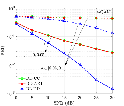
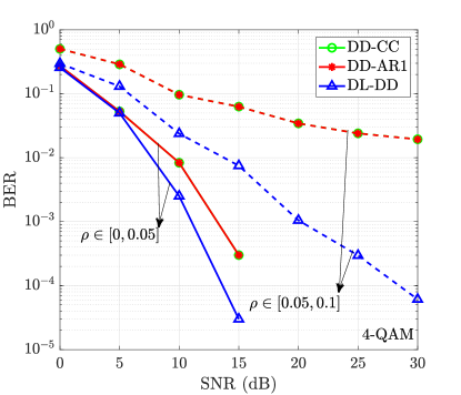
In this section we provide some performance measures to compare our proposed DL-based DD-CE for MIMO communication systems with the DD-CE method which model channel based on first order autoregressive model in [28] and the MMSE DD-CE provided in [29] where channel is assumed to be coherent for each of STBC block transmission. We denote our method by DL-DD and the methods in [28] and [29] by DD-AR1 and DD-CC, respectively.
VII-A Simulation Setup
Unless otherwise mentioned, we consider 4-QAM constellation in MIMO time-varying fading channel and run our simulations for both Rayleigh and Rician fading channels. We model the fading channels by Jake’s Doppler spectrum, where the autocorrelation function of the channel is given as
| (57) | ||||
with being -factor, being line-of-sight (LOS) component of fading, being the average non-line-of-sight (NLOS) power of , and being the Doppler rate. Without loss of generality, we assume that the only available knowledge in the receiver side is the range of Doppler rate and not the exact value which is accessible by current channel estimators. The range of Doppler rate is set such that .
We provide performance measures for three different STBCs including Alamouti STBC [25] which gives a rate one by transmit antennas as
| (58) |
Tarokh et. al’s STBC [26] which achieves code rate with transmit antennas given by
| (59) |
and the following STBC code with code rate with , , and as
| (60) |
The additive noise is modeled as circular symmetric zero-mean complex-valued Gaussian random variable with variance , i.e. . The signal-to-noise ratio (SNR) in dB is defined as , where is the average transmitted power. Unless otherwise mentioned, the length of the transmitted packet is and the length of the pilot is and also .
We use a training set of size to learn the two predictor functions in (31). The details about the training phase parameters are included in Table IV.
| Parameter | Value |
|---|---|
| Number of batches | |
| Size of batches | 10 |
| Number of epoches | 2000 |
| Number of iterations |
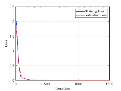
Adam optimizer [32] with learning rate of was used for loss function minimization. Fig. (2) compares the training loss and validation loss during the training phase at dB SNR. As seen, the gap between the training and validation loss diminishes when the DNN is trained for more iterations.
For a range of different SNRs and Doppler rates, we run Monte Carlo iterations to reach to a fair comparison between the existing channel estimator algorithms in terms of BER. At each simulation setup we assume that the exact Doppler rate is known when DD-AR1 and DD-CC algorithms are employed while only the range of Doppler rate is known for the DL-DD algorithm.
VII-B Simulation Results
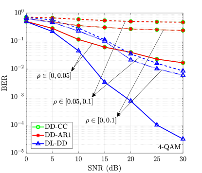
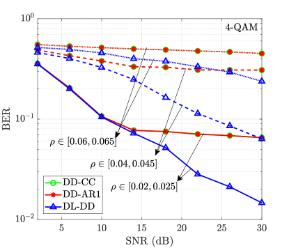
The performance of the DL-DD, DD-AR1 and DD-CC algorithms have been studied, and they have employed in different ranges of Doppler rates. Fig. 3, Fig. 4 and Fig. 5 shows the performance comparison between these algorithms for Alamouti’s STBC, Tarokh et. al.’s STBC and STBC in (60), respectively for a Rayleigh channel. It is obvious from these figures that our proposed algorithm dramatically outperform the DD-AR1 and DD-CC algorithms at any SNRs and Doppler ranges in both cases even without the knowledge of the Doppler rate. As expected, increasing the SNR results in lower BER and this reduction in BER is more considerable in our algorithm. We repeat this simulation for a Rician channel with Alamouti’s STBC and provide the results in Fig. 6. As seen, again our DL-DD algorithm outperforms the DD-AR1 and DD-CC algorithms.
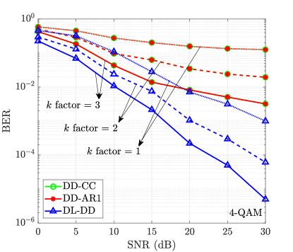
One of the parameters of a Rician channel that could affect the performance is factor. We study the effect of factor on the achieved BER by our DL-DD algorithm for Alamouti’s STBC and provide it in Fig. 7. It is obvious from the figure that the performance of our DL-DD algorithm is considerably better than DD-CC and DD-AR1 algorithms and as the value of -factor increases we obtain better BER with all the algorithms.
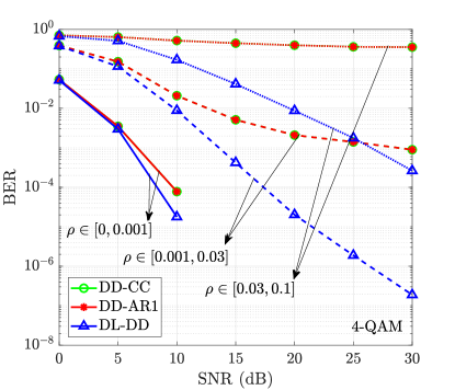
In order to study the effect of moving object’s speed on the performance of the channel predictors, we define three distinct Doppler rate ranges based on the speed of moving objects and provide a comparison in the following. We have the following equation for the relation between Doppler rate and moving object’s speed as
| (61) |
where is the carrier frequency which is typically in the order of 10 GHz in 5G [4], is the sampling time, and is the speed of light, i.e. m/s. We consider three Doppler rate ranges for pedestrians, cars and high speed trains as in Table V.
| Name | Speed (m/s) | Doppler Rate Range |
|---|---|---|
| Pedestrians | m/s | |
| Cars | m/s | |
| High Speed Trains | m/s |
Fig.8 shows the performance comparison between DL-DD, DD-AR1 and DD-CC for Alamouti’s STBC and the Doppler rate ranges in Table V. As seen, our proposed DL-DD algorithm outperforms DD-AR1 and DD-CC in terms of BER.
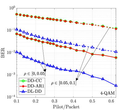
We study the effect of packet length on BER and show the BER versus for and at dB for Alamouti’s STBC in Fig. 9. It is assumed that the channel is in Rayleigh distribution and and the number of STBC transmission block, , varies. As seen, the proposed DL-DD algorithm improves transmission reliability for long packets compared to the DD-AR1 and DD-CC algorithms. The reason is that the channel prediction error in the DL-DD algorithm is much lower that the one in the other algorithms. The lower prediction error in the DL-DD algorithm leads to lower propagation error.
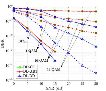
The effect of modulation format on the performance of the proposed DL-based DD-CE algorithm for Alamouti’s STBC in Rayleigh fading channel is shown in Fig. 10. As seen, our proposed algorithm outperforms the other algorithms in terms of BER. Also, as modulation order increases, the BER increases.
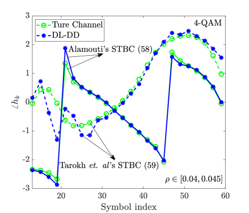
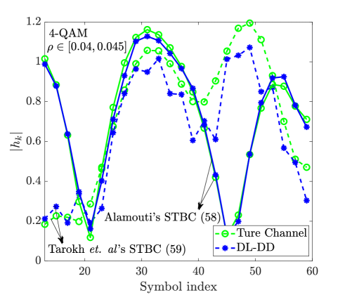
Channel tracking capability of our proposed DL-based algorithm in Rayleigh fading channel for Alamouti’s STBC is presented in Fig. 11. As seen, the amplitude and phase of the predicted channels by the proposed DL-DD algorithm is very close to the true channel for a packet transmission of length .
VIII Conclusion
The acmimo communication systems enable us to achieve a higher data rate even in highly dynamic environments. However, this requires an improved CE algorithm to be functional even in fast fading channels. In this paper we study DD-CE algorithm and develop a new DL-based DD-CE algorithm to track fading channels and detect data for longer packets even in rapid vehicular environments. We also derive the ML decoding formula for STBC transmission. Our algorithm benefits from a simple receiver design which does not rely on the accurate statistical model of the fading channel and only the range of Doppler rate is sufficient. This capability removes the need for Doppler spread estimation, which is considerably challenging for highly dynamic vehicular environments. We compare our algorithm with DD-AR1 and DD-CC algorithms through several performance measures and it outperforms existing algorithms while the DD-AR1 and DD-CC know the exact value of Doppler rate.
Acknowledgment
The study presented in this paper is supported in part by the Huawei Innovation Research Program (HIRP).
References
- [1] “Cisco visual networks index: Global mobile data traffic forecast update 2016–2021,” CISCO White papers, 2017.
- [2] J. Gubbi, R. Buyya, S. Marusic, and M. Palaniswami, “Internet of things (IoT): A vision, architectural elements, and future directions,” Future Generation Computer Systems, vol. 29, no. 7, pp. 1645 – 1660, 2013. [Online]. Available: http://www.sciencedirect.com/science/article/pii/S0167739X13000241
- [3] T. S. Rappaport, Y. Xing, G. R. MacCartney, A. F. Molisch, E. Mellios, and J. Zhang, “Overview of millimeter wave communications for fifth-generation (5g) wireless networks with a focus on propagation models,” IEEE Transactions on Antennas and Propagation, vol. 65, no. 12, pp. 6213–6230, Dec 2017.
- [4] T. S. Rappaport, S. Sun, R. Mayzus, H. Zhao, Y. Azar, K. Wang, G. N. Wong, J. K. Schulz, M. Samimi, and F. Gutierrez, “Millimeter wave mobile communications for 5g cellular: It will work!” IEEE Access, vol. 1, pp. 335–349, 2013.
- [5] S. Sun, T. S. Rappaport, R. W. Heath, A. Nix, and S. Rangan, “MIMO for millimeter-wave wireless communications: beamforming, spatial multiplexing, or both?” IEEE Communications Magazine, vol. 52, no. 12, pp. 110–121, December 2014.
- [6] J. G. Andrews, S. Buzzi, W. Choi, S. V. Hanly, A. Lozano, A. C. K. Soong, and J. C. Zhang, “What will 5g be?” IEEE Journal on Selected Areas in Communications, vol. 32, no. 6, pp. 1065–1082, June 2014.
- [7] A. Adhikary, E. A. Safadi, M. K. Samimi, R. Wang, G. Caire, T. S. Rappaport, and A. F. Molisch, “Joint spatial division and multiplexing for mm-wave channels,” IEEE Journal on Selected Areas in Communications, vol. 32, no. 6, pp. 1239–1255, June 2014.
- [8] R. B. Ertel, P. Cardieri, K. W. Sowerby, T. S. Rappaport, and J. H. Reed, “Overview of spatial channel models for antenna array communication systems,” IEEE Personal Communications, vol. 5, no. 1, pp. 10–22, Feb 1998.
- [9] R. He, B. Ai, G. L. Stüber, and Z. Zhong, “Mobility model-based non-stationary mobile-to-mobile channel modeling,” IEEE Transactions on Wireless Communications, vol. 17, no. 7, pp. 4388–4400, July 2018.
- [10] P. Fan, E. Panayirci, H. V. Poor, and P. T. Mathiopoulos, “Special issue on broadband mobile communications at very high speeds,” EURASIP Journal on Wireless Communications and Networking, vol. 2012, no. 1, p. 279, Aug 2012. [Online]. Available: https://doi.org/10.1186/1687-1499-2012-279
- [11] K. Shi, E. Serpedin, and P. Ciblat, “Decision-directed fine synchronization in OFDM systems,” IEEE Transactions on Communications, vol. 53, no. 3, pp. 408–412, March 2005.
- [12] E. Karami and M. Shiva, “Decision-directed recursive least squares mimo channels tracking,” EURASIP Journal on Wireless Communications and Networking, vol. 2006, no. 1, p. 043275, 2006.
- [13] X. Deng, A. M. Haimovich, and J. Garcia-Frias, “Decision directed iterative channel estimation for mimo systems,” in Communications, 2003. ICC ’03. IEEE International Conference on, vol. 4, May 2003, pp. 2326–2329 vol.4.
- [14] H. Ye, G. Y. Li, and B.-H. Juang, “Power of deep learning for channel estimation and signal detection in OFDM systems,” IEEE Wireless Communications Letters, vol. 7, no. 1, pp. 114–117, 2018.
- [15] E. Nachmani, E. Marciano, L. Lugosch, W. J. Gross, D. Burshtein, and Y. Be’ery, “Deep learning methods for improved decoding of linear codes,” IEEE Journal of Selected Topics in Signal Processing, 2018.
- [16] N. Farsad and A. Goldsmith, “Detection algorithms for communication systems using deep learning,” arXiv preprint arXiv:1705.08044, 2017.
- [17] M. Kim, N.-I. Kim, W. Lee, and D.-H. Cho, “Deep learning aided SCMA,” IEEE Communications Letters, 2018.
- [18] T. O’Shea and J. Hoydis, “An introduction to deep learning for the physical layer,” IEEE Transactions on Cognitive Communications and Networking, vol. 3, no. 4, pp. 563–575, 2017.
- [19] S. Dörner, S. Cammerer, J. Hoydis, and S. ten Brink, “Deep learning based communication over the air,” IEEE Journal of Selected Topics in Signal Processing, vol. 12, no. 1, pp. 132–143, 2018.
- [20] T. J. O’Shea, T. Erpek, and T. C. Clancy, “Deep learning based MIMO communications,” arXiv preprint arXiv:1707.07980, 2017.
- [21] M. Mohammadkarimi, M. Mehrabi, M. Ardakani, and Y. Jing, “Deep learning based sphere decoding,” IEEE Transactions on Wireless Communications, Submitted, June 2018.
- [22] I. Goodfellow, Y. Bengio, A. Courville, and Y. Bengio, Deep learning. MIT press Cambridge, 2016, vol. 1.
- [23] C. Komninakis, C. Fragouli, A. H. Sayed, and R. D. Wesel, “Multi-input multi-output fading channel tracking and equalization using Kalman estimation,” IEEE Transactions on Signal Processing, vol. 50, no. 5, pp. 1065–1076, May 2002.
- [24] B. D. Anderson and J. B. Moore, “Optimal filtering,” Englewood Cliffs, vol. 21, pp. 22–95, 1979.
- [25] S. M. Alamouti, “A simple transmit diversity technique for wireless communications,” IEEE J. Sel. Areas Commun., vol. 16, no. 8, pp. 1451–1458, Oct 1998.
- [26] V. Tarokh, H. Jafarkhani, and A. R. Calderbank, “Space-time block codes from orthogonal designs,” IEEE Transactions on Information Theory, vol. 45, no. 5, pp. 1456–1467, July 1999.
- [27] Z. Liu, X. Ma, and G. B. Giannakis, “Space-time coding and Kalman filtering for time-selective fading channels,” IEEE Transactions on Communications, vol. 50, no. 2, pp. 183–186, Feb 2002.
- [28] Z. Liu, G. B. Giannakis, and B. L. Hughes, “Double differential space-time block coding for time-selective fading channels,” IEEE Transactions on Communications, vol. 49, no. 9, pp. 1529–1539, 2001.
- [29] V. Tarokh and H. Jafarkhani, “A differential detection scheme for transmit diversity,” IEEE Journal on Selected Areas in Communications, vol. 18, no. 7, pp. 1169–1174, July 2000.
- [30] B. Balakumar, S. Shahbazpanahi, and T. Kirubarajan, “Joint MIMO channel tracking and symbol decoding using Kalman filtering,” IEEE Transactions on Signal Processing, vol. 55, no. 12, pp. 5873–5879, Dec 2007.
- [31] F. Hlawatsch and G. Matz, Wireless communications over rapidly time-varying channels. Academic Press, 2011.
- [32] D. P. Kingma and J. Ba, “Adam: A method for stochastic optimization,” arXiv preprint arXiv:1412.6980, 2014.