Preventing posterior collapse with $\delta$-VAEs

Abstract

Due to the phenomenon of “posterior collapse,” current latent variable generative models pose a challenging design choice that either weakens the capacity of the decoder or requires augmenting the objective so it does not only maximize the likelihood of the data. In this paper, we propose an alternative that utilizes the most powerful generative models as decoders, whilst optimising the variational lower bound all while ensuring that the latent variables preserve and encode useful information. Our proposed $\delta$-VAEs achieve this by constraining the variational family for the posterior to have a minimum distance to the prior. For sequential latent variable models, our approach resembles the classic representation learning approach of slow feature analysis. We demonstrate the efficacy of our approach at modeling text on LM1B and modeling images: learning representations, improving sample quality, and achieving state of the art log-likelihood on CIFAR-10 and ImageNet $32\times 32$.

1 Introduction

Deep latent variable models trained with amortized variational inference have led to advances in representation learning on high-dimensional datasets (Kingma & Welling, 2013; Rezende et al., 2014). These latent variable models typically have simple decoders, where the mapping from the latent variable to the input space is uni-modal, for example using a conditional Gaussian decoder. This typically results in representations that are good at capturing the global structure in the input, but fail at capturing more complex local structure (e.g., texture (Larsen et al., 2016)). In parallel, advances in autoregressive models have led to drastic improvements in density modeling and sample quality without explicit latent variables (van den Oord et al., 2016b). While these models are good at capturing local statistics, they often fail to produce globally coherent structures (Ostrovski et al., 2018).

Combining the power of tractable densities from autoregressive models with the representation learning capabilities of latent variable models could result in higher-quality generative models with useful latent representations. While much prior work has attempted to join these two models, a common problem remains. If the autoregressive decoder is expressive enough to model the data density, then the model can learn to ignore the latent variables, resulting in a trivial posterior that collapses to the prior. This phenomenon has been frequently observed in prior work and has been referred to as optimisation challenges of VAEs by Bowman et al. (2015), the information preference property by Chen et al. (2016), and the posterior collapse problems by several others (e.g., van den Oord et al. (2017); Kim et al. (2018)). Ideally, an approach that mitigates posterior collapse would not alter the evidence lower bound (ELBO) training objective, and would allow the practitioner to leverage the most recent advances in powerful autoregressive decoders to improve performance. To the best of our knowledge, no prior work has succeeded at this goal. Most common approaches either change the objective (Higgins et al., 2017; Alemi et al., 2017; Zhao et al., 2017; Chen et al., 2016; Lucas & Verbeek, 2017), or weaken the decoder (Bowman et al., 2015; Gulrajani et al., 2016). Additionally, these approaches are often challenging to tune and highly sensitive to hyperparameters (Alemi et al., 2017; Chen et al., 2016).

In this paper, we propose $\delta$-VAEs, a simple framework for selecting variational families that prevent posterior collapse without altering the ELBO training objective or weakening the decoder. By restricting the parameters or family of the posterior, we ensure that there is a minimum KL divergence, $\delta$, between the posterior and the prior.

We demonstrate the effectiveness of this approach at learning latent-variable models with powerful decoders on images (CIFAR-10, and ImageNet $32\times 32$), and text (LM1B). We achieve state of the art log-likelihood results with image models by additionally introducing a sequential latent-variable model with an anti-causal encoder structure. Our experiments demonstrate the utility of $\delta$-VAEs at learning useful representations for downstream tasks without sacrificing performance on density modeling.

2 Mitigating posterior collapse with $\delta$-VAEs

Our proposed $\delta$-VAE builds upon the framework of variational autoencoders (VAEs) (Kingma & Welling, 2013; Rezende et al., 2014) for training latent-variable models with amortized variational inference. Our goal is to train a generative model $p(x,z)$ to maximize the marginal likelihood $\log p(x)$ on a dataset. As the marginal likelihood requires computing an intractable integral over the unobserved latent variable $z$, VAEs introduce an encoder network $q(z|x)$ and optimize a tractable lower bound (the ELBO): $\log p(x)\geq\mathbb{E}_{z\sim q(z|x)}\left[\log p(x|z)\right]-D_{\mathrm{KL}}(q(z|x)\|p(z))$. The first term is the reconstruction term, while the second term (KL) is the rate term, as it measures how many nats on average are required to send through the latent variables from the encoder ($q(z|x)$) to the decoder ($p(z|x)$) (Hoffman et al., 2016; Alemi et al., 2017).

The problem of posterior collapse is that the rate term, $D_{\mathrm{KL}}(q(z|x)\|p(z))$ reduces to 0. In this case, the approximate posterior $q(z|x)$ equals the prior $p(z)$, thus the latent variables do not convey any information about the input $x$. A necessary condition if we want representations to be meaningful is to have the rate term be positive.

In this paper we address the posterior collapse problem with structural constraints so that the KL divergence between the posterior and prior is lower bounded by design. This can be achieved by choosing families of distributions for the prior and approximate posterior, $p_{\theta}({\mathbf{z}})$ and $q_{\phi}({\mathbf{z}}|{\mathbf{x}})$ such that $\min_{\theta,\phi}D_{\mathrm{KL}}(q_{\phi}({\mathbf{z}}|{\mathbf{x}})\|p_{\theta}({\mathbf{z}}))\geq\delta$. We refer to $\delta$ as the committed rate of the model.

Note that a trivial choice for $p$ and $q$ to have a non-zero committed rate is to set them to Gaussian distributions with fixed (but different) variance term. We study a variant of this case in the experiments, and provide more details of this setup in Appendix D. In the following section we describe our choices for $p_{\theta}$ and $q_{\phi}$ , but others should also be explored in future work.

2.1 $\delta$-VAE with Sequential Latent Variables

Data such as speech, natural images and text exhibit strong spatio-temporal continuity. Our aim is to model variations in such data through latent variables, so that we have control over not just the global characteristics of the generated samples (e.g., existence of an object), but also can influence their finer, often shifting attributes such as texture and pose in the case of natural images, tone, volume and accent in the case of speech, or style and sentiment in the case of natural language. Sequences of latent variables can be an effective modeling tool for expressing the occurrence and evolution of such features throughout the sequence.

To construct a $\delta$-VAE in the sequential setting, we combine a mean field posterior with a correlated prior in time. We model the posterior distribution of each timestep as $q({\mathbf{z}}_{t}|{\mathbf{x}})=\mathcal{N}({\mathbf{z}}_{t};\mu_{t}({\mathbf{x}}),\sigma_{t}({\mathbf{x}}))$. For the prior, we use an first-order linear autoregressive process (AR(1)), where ${\mathbf{z}}_{t}=\alpha{\mathbf{z}}_{t-1}+\epsilon_{t}$ with $\epsilon_{t}$ zero mean Gaussian noise with constant variance $\sigma_{\epsilon}^{2}$. The conditional probability for the latent variable can be expressed as $p({\mathbf{z}}_{t}|{\mathbf{z}}_{<t})=\mathcal{N}({\mathbf{z}}_{t};\alpha{\mathbf{z}}_{t-1},\sigma_{\epsilon})$. This process is wide-sense stationary (that is, having constant sufficient statistics through its time evolution) if $|\alpha|<1$. If so, then ${\mathbf{z}}_{t}$ has zero mean and variance of $\frac{\sigma_{\epsilon}^{2}}{1-\alpha^{2}}$. It is thus convenient to choose $\sigma_{\epsilon}=\sqrt{1-\alpha^{2}}$. The mismatch in the correlation structure of the prior and the posterior results in the following positive lower bound on the KL-divergence between the two distributions (see Appendix C for derivation):

$$D_{\mathrm{KL}}(q({\mathbf{z}}|{\mathbf{x}})\|p({\mathbf{z}}))\geq\frac{1}{2}\sum_{k=1}^{d}(n-2)\ln(1+\alpha_{k}^{2})-\ln(1-\alpha_{k}^{2})$$ (1)

where $n$ is the length of the sequence and $d$ is the dimension of the latent variable at each timestep. The committed rate between the prior and the posterior is easily controlled by equating the right hand side of the inequality in equation 1 to a given rate $\delta$ and solving for $\alpha$. In Fig. 1, we show the scaling of the minimum rate as a function of $\alpha$ and the behavior of $\delta$-VAE in 2d.

Figure 1: Effect of $\delta$ in a toy model. Fitting an uncorrelated Gaussian for the posterior, $q_{\phi}(z)$, to a correlated Gaussian prior, $p_{\alpha}(z)$, by minimizing $D_{\mathrm{KL}}(q_{\phi}(z)\|p_{\alpha}(z))$ over $\phi$. Left: committed rate ($\delta)$ as a function of the prior squared correlation $\alpha$ and the dimensionality $n$. Right: contours of the optimal posterior and prior in 2d. As the correlation increases, the minimum rate grows.

2.1.1 Relation to Probabilistic Slowness Prior

The AR(1) prior over the latent variables specifies the degree of temporal correlation in the latent space. As the correlation $\alpha$ approaches one, the prior trajectories get smoother . On the other hand in the limit of $\alpha$ approaching $0$, the prior becomes the same as the independent standard Gaussian prior where there are no correlations between timesteps. This pairing of independent posterior with a correlated prior is related to the probabilistic counterpart to Slow Feature Analysis (Wiskott & Sejnowski, 2002) in Turner & Sahani (2007). SFA has been shown to be an effective method for learning invariant spatio-temporal features (Wiskott & Sejnowski, 2002). In our models, we infer latent variables with multiple dimensions per timestep, each with a different slowness filter imposed by a different value of $\alpha$, corresponding to features with different speed of variation.

2.2 Anti-Causal Encoder Network

Having a high capacity autoregressive network as the decoder implies that it can accurately estimate $p({\mathbf{x}}_{t}|{\mathbf{x}}_{<t})$. Given this premise, what kind of complementary information can latent variables provide? Encoding information about the past seems wasteful as the autoregressive decoder has full access to past observations already. On the other hand, if we impose conditional independence between observations and latent variables at other timesteps given the current one (i.e., $p({\mathbf{x}}_{t}|{\mathbf{z}})=p({\mathbf{x}}_{t}|{\mathbf{z}}_{t})$), there will then be at best (by the data processing inequality (Cover & Thomas, 2006)) a break-even situation between the KL cost of encoding information in ${\mathbf{z}}_{t}$ and the resulting improvement in the reconstruction loss. There is therefore no advantage for the model to utilize the latent variable even if it would transmit to the decoder the unobserved ${\mathbf{x}}_{t}$. The situation is different when ${\mathbf{z}}_{t}$ can inform the decoder at multiple timesteps, encoding information about ${\mathbf{x}}_{t}$ and ${\mathbf{x}}_{>t}$. In this setting, the decoder pays the KL cost for the mutual information once, but is able to leverage the transmitted information multiple times to reduce its entropy about future predictions.

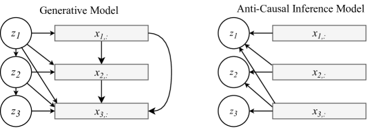
To encourage the generative model to leverage the latents for future timesteps, we introduce an anti-causal structure for the encoder where the parameters of the variational posterior for a timestep cannot depend on past observations (Fig. 2). Alternatively, one can consider a non-causal structure that allows latents be inferred from all observations. In this non-causal setup there is no temporal order in either the encoder or the decoder, thus the model resembles a standard non-temporal latent variable model. While the anti-causal structure is a subgraph of the non-causal structure, we find that the anti-causal structure often performs better, and we compare both approaches in different settings in Appendix F.1.

Figure 2: Generative structures for the inference of sequential latent variables. The anti-causal structure introduces an inductive bias to encode in each latent variable information about the future

3 Related Work

The main focus of our work is on representation learning and density modeling in latent variable models with powerful decoders. Earlier work has focused on this kind of architecture, but has addressed the problem of posterior collapse in different ways.

In terms of our architecture, the decoders for our image models build on advances in autoregressive modeling from van den Oord et al. (2016b); Salimans et al. (2017); Chen et al. (2017); Parmar et al. (2018). Unlike prior models, we use sequential latent variables to generate the image row by row. This differs from Gregor et al. (2016), where the latent variables are sequential but the entire image is generated at each timestep. Our sequential image generation model resembles latent variable models used for timeseries (Chung et al., 2015; Babaeizadeh et al., 2017; Denton & Fergus, 2018) but does not rely on KL annealing, and has an additional autoregressive dependence of the outputs over time (rows of the image). Another difference between our work and previous sequential latent variable models is our proposed anti-causal structure for the inference network (see Sect. 2.2). We motivate this structure from a coding efficiency and representation learning standpoint and demonstrate its effectiveness empirically in Sect. 4. For textual data, we use the Transformer architecture from Vaswani et al. (2017) as our main blueprint for the decoder. As shown in Sect. 4, our method is able to learn informative latent variables while preserving the performance of these models in terms of likelihoods.

To prevent posterior collapse, most prior work has focused on modifying the training objective. Bowman et al. (2015); Yang et al. (2017); Kim et al. (2018) and Gulrajani et al. (2016) use an annealing strategy, where they anneal the weight on the rate from 0 to 1 over the course of training. This approach does not directly optimize a lower bound on likelihood for most of training, and tuning the annealing schedule to prevent collapse can be challenging (see Sect. 4). Similarly, Higgins et al. (2017) proposes using a fixed coefficient $>1$ on the rate term to learn disentangled representations. Zhao et al. (2017) adds a term to the objective to pick the model with maximal rate. Chen et al. (2016); Kingma et al. (2016) use free-bits to allow the model to hit a target minimum rate, but the objective is non-smooth which leads to optimization difficulties in our hands, and deviations from a lower bound on likelihood when the soft version is used with a coefficient less than 1. Lucas & Verbeek (2017) add an auxiliary objective that reconstructs a low-resolution version of the input to prevent posterior collapse. Alemi et al. (2017) argue that the ELBO is a defective objective function for representation learning as it does not distinguish between models with different rates, and advocate for model selection based on downstream tasks. Their method for sweeping models was to use $\beta$-VAE with different coefficients, which can be challenging as the mapping from $\beta$ to rate is highly nonlinear, and model- and data-dependent. While we adopt the same perspective as Alemi et al. (2017), we present a new way of achieving a target rate while optimizing the vanilla ELBO objective.

Most similar to our approach is work on constraining the variational family to regularize the model. VQ-VAE (van den Oord et al., 2017) uses discrete latent variables obtained by vector quantization of the latent space that, given a uniform prior over the outcome, yields a fixed KL divergence equal to $\log K$, where $K$ is the size of the codebook. A number of recent papers have also used the von Mises-Fisher (vMF) distribution to obtain a fixed KL divergence and mitigate the posterior collapse problem. In particular, Guu et al. (2017); Xu & Durrett (2018); Davidson et al. (2018) use vMF($\mu,\kappa$) with a fixed $\kappa$ as their posterior, and the uniform distribution (i.e. vMF($\cdot$, 0)) as the prior. The mismatching prior-posterior thus give a constant KL divergence. As such, this approach can be considered as the continuous analogue of VQ-VAE. Unlike the VQ-VAE and vMF approaches which have a constant KL divergence for every data point, $\delta$-VAE can allow higher KL for different data points. This allows the model to allocate more bits for more complicated inputs, which has been shown to be useful for detecting outliers in datasets (Alemi et al., 2018). As such, $\delta$-VAE may be considered a generalisation of these fixed-KL approaches.

The Associative Compression Networks (ACN) (Graves & Menick, 2014) is a new method for learning latent variables with powerful decoders that exploits the associations between training examples in the dataset by amortizing the description length of the code among many similar training examples. ACN deviates from the i.i.d training regime of the classical methods in statistics and machine learning, and is considered a procedure for compressing whole datasets rather than individual training examples. GECO (Jimenez Rezende & Viola, 2018) is a recently proposed method to stabilize the training of $\beta$-VAEs by finding an automatic annealing schedule for the KL that satisfies a tolerance constraint for maximum allowed distortion, and solving the resulting Lagrange multiplier for the KL penalty. The value of $\beta$, however, does not necessarily approach one, which means that the optimized objective may not be a lower bound for the marginal likelihood.

4 Experiments

4.1 Natural Images

We applied our method to generative modeling of images on the CIFAR-10 (Krizhevsky et al., ) and downsampled ImageNet (Deng et al., 2009) ($32\times 32$ as prepared in PixelRNN) datasets. We describe the main components in the following. The details of our hyperparameters can be found in Appendix E.

Decoder: Our decoder network is closest to PixelSNAIL (PixelSnail) but also incorporates elements from the original GatedPixelCNN (pixelcnn). In particular, as introduced by PixelCNN++ and used in PixelSnail, we use a single channel network to output the components of discretised mixture of logistics distributions for each channel, and linear dependencies between the RGB colour channels. As in PixelSNAIL, we use attention layers interleaved with masked gated convolution layers. We use the same architecture of gated convolution introduced in pixelcnn. We also use the multi-head attention module of Vaswani2017. To condition the decoder, similar to Transformer and unlike PixelCNN variants that use 1x1 convolution, we use attention over the output of the encoder. The decoder-encoder attention is causally masked to realize the anti-causal inference structure, and is unmasked for the non-causal structure.

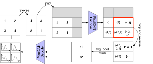
Encoder. Our encoder also uses the same blueprint as the decoder. To introduce the anti-causal structure the input is reversed, shifted and cropped by one in order to obtain the desired future context. Using one latent variable for each pixel is too inefficient in terms of computation so we encode each row of the image with a multidimensional latent variable.

Auxiliary Prior. vamprior; Hoffman2016; Geco show that VAE performance can suffer when there is a significant mismatch between the prior and the aggregate posterior, $q(z)=\mathbb{E}_{x\sim\mathcal{D}}\left[q(z|x)\right]$. When such a gap exists, the decoder is likely to have never seen samples from regions of the prior distribution where the aggregate posterior assigns small probability density. This phenomenon, also known as the “posterior holes” problem (Geco), can be exacerbated in $\delta$-VAEs, where the systematic mismatch between the prior and the posterior might induce a large gap between the prior and aggregate posterior. Increasing the complexity of the variational family can reduce this gap (NF), but require changes in the objective to control the rate and prevent posterior collapse (IAF). To address this limitation, we adopt the approaches of VQVAE; roy2018theory and train an auxiliary prior over the course of learning to match the aggregate posterior, but that does not influence the training of the encoder or decoder. We used a simple autoregressive model for the auxiliary prior $p^{aux}$: a single-layer LSTM network with conditional-Gaussian outputs.

4.1.1 Density Estimation Results

We begin by comparing our approach to prior work on CIFAR-10 and downsampled ImageNet 32x32 in Table 1. As expected, we found that the capacity of the employed autoregressive decoder had a large impact on the overall performance. Nevertheless, our models with latent variables have a negligible gap compared to their powerful autoregressive latent-free counterparts, while also learning informative latent variables. In comparison, (VLAE) had a 0.03 bits per dimension gap between their latent variable model and PixelCNN++ architecture. On ImageNet 32x32, our latent variable model achieves on par performance with purely autoregressive Image Transformer (ImageTransformer). On CIFAR-10 we achieve a new state of the art of 2.83 bits per dimension, again matching the performance of our autoregressive baseline. Note that the values for KL appear quite small as they are reported in bits per dimension (e.g. 0.02 bits/dim translates to 61 bits/image encoded in the latents). The results on CIFAR-10 also demonstrate the effect of the auxiliary prior on improving the efficiency of the latent code; it leads to more than $50\%$ (on average 30 bits per image) reduction in the rate of the model to achieve the same performance.

	CIFAR-10 Test	ImageNet $32\times 32$ Valid
Latent Variable Models
ConvDraw (ConvDraw)	$\leq$ 3.85	-
DenseNet VLAE (VLAE)	$\approx$ 2.95	-
$\delta$-VAE + PixelSNAIL + AR(1) Prior	$\leq$ 2.85 (0.02)	$\leq$ 3.78 (0.08)
$\delta$-VAE + PixelSNAIL + Auxiliary Prior	$\leq$ 2.83 (0.01)	$\leq$ 3.77 (0.07)
Autoregressive Models
Gated PixelCNN(pixelcnn)	3.03	3.83
PixelCNN++ (PixelCNN++)	2.92	-
PixelRNN (PixelRNN)	3.00	-
ImageTransformer (ImageTransformer)	2.90	3.77
PixelSNAIL (PixelSnail)	2.85	3.80
Our Decoder baseline	2.83	3.77

Table 1: Estimated upper bound on negative log-likelihood along with KL-divergence (in parenthesis) in bits per dimension for CIFAR-10 and downsampled ImageNet.

4.2 Utilization of Latent Variables

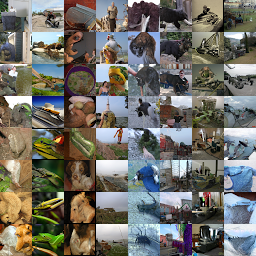
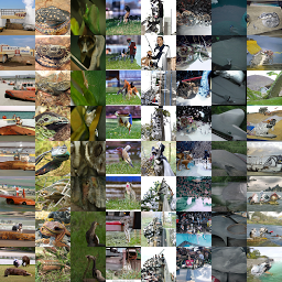
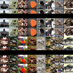
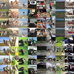
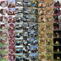
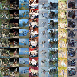
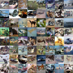
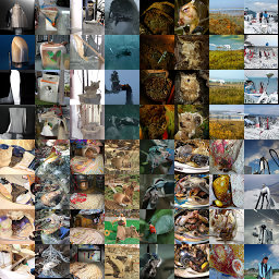
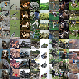
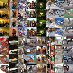
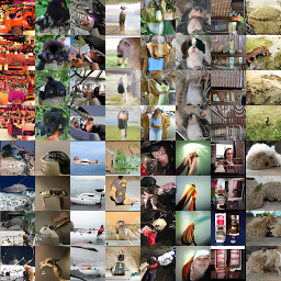
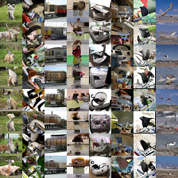
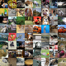
In this section, we aim to demonstrate that our models learn meaningful representations of the data in the latent variables. We first investigate the effect of ${\mathbf{z}}$ on the generated samples from the model. Fig. 3 depicts samples from an ImageNet model (see Appendix for CIFAR-10), where we sample from the decoder network multiple times conditioned on a fixed sample from the auxiliary prior. We see similar global structure (e.g. same color background, scale and structure of objects) but very different details. This indicates that the model is using the latent variable to capture global structure, while the autoregressive decoder is filling in local statistics and patterns.

(a) Multiple decoding of the same ${\mathbf{z}}$

(b) Random samples from the our Auxiliary prior

Figure 3: Random samples from our ImageNet $32\times 32$ model. Each column in Fig. 3(a) shows multiple samples from $p({\mathbf{x}}|{\mathbf{z}})$ for a fixed ${\mathbf{z}}\sim p_{aux}({\mathbf{z}})$. Each image in Fig. 3(b) is decoded using a different sample from $p_{aux}({\mathbf{z}})$.

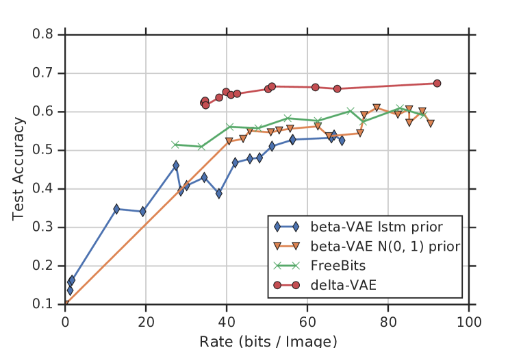
For a more quantitative assessment of how useful the learned representations are for downstream tasks, we performed linear classification from the representation to the class labels on CIFAR-10. We also study the effect of the chosen rate of the model on classification accuracy as illustrated in Fig. 4(b), along with the performance of other methods. We find that generally a model with higher rate gives better classification accuracy, with our highest rate model, encoding 92 bits per image, giving the best accuracy of $68\%$. However, we find that improved log-likelihood does not necessarily lead to better linear classification results. We caution that an important requirement for this task is the linear separability of the learned feature space, which may not align with the desire to learn highly compressed representations.

4.3 Ablation studies

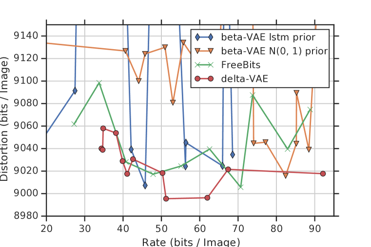
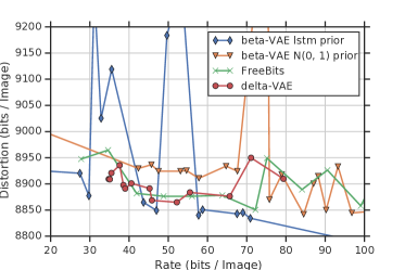
We performed more extensive comparisons of $\delta$-VAE with other approaches to prevent posterior collapse on the CIFAR-10 dataset. We employ the same medium sized encoder and decoder for evaluating all methods as detailed in Appendix E. Fig. 4(a) reports the rate-distortion results of our experiments for the CIFAR-10 test set. To better highlight the difference between models and to put into perspective the amount of information that latent variables capture about images, the rate and distortion results in Fig. 4(a) are reported in bits per images. We only report results for models that encode a non-negligible amount information in latent variables. Unlike the committed information rate approach of $\delta$-VAE, most alternative solutions required considerable amount of effort to get the training converge or prevent the KL from collapsing altogether. For example, with linear annealing of KL (Bowman2015), despite trying a wide range of values for the end step of the annealing schedule, we were not able to train a model with a significant usage of latent variables; the KL collapsed as soon as $\beta$ approached 1.0. A practical advantage of our approach is its simple formula to choose the target minimum rate of the model. Targeting a desired rate in $\beta$-VAE, on the other hand, proved to be difficult, as many of our attempts resulted in either collapsed KL, or very large KL values that led to inefficient inference. As reported in VLAE, we also observed that optimising models with the free-bits loss was challenging and sensitive to hyperparameter values.

To assess each methods tendency to overfit across the range of rates, we also report the rate-distortion results for CIFAR-10 training sets in  Appendix F. While beta-VAEs do find points along the rate-distortion optimal frontier on the training set, we found that they overfit more than delta-VAEs, with delta-VAEs dominating the rate-distortion frontier on heldout data.

(a) Rate-Distortion

(b) Rate vs. Classification Accuracy

Figure 4: Comparison of CIFAR-10 test performance of $\delta$-VAEs vs. models trained with free-bits and $\beta$-VAE across many rates. $\delta$-VAE is significantly more stable, achieves competitive density estimation results across different rates, and its learned representations perform better in the downstream linear classification task.

Next, we compare the performance of the anti-causal encoder structure with the non-causal structure on the CIFAR-10 dataset discussed in Sect. 2.2. The results for several configurations of our model are reported in the Appendix Table 6. In models where the decoder is not powerful enough (such as our 6-layer PixelCNN that has no attention and consequently a receptive field smaller than the causal context for most pixels), the anti-causal structure does not perform as well as the non-causal structure. The performance gap is however closed as the decoder becomes more powerful and its receptive field grows by adding self-attention and more layers. We observed that the anti-causal structure outperforms the non-causal encoder for very high capacity decoders, as well as for medium size models with a high rate. We also repeated these experiments with both anti-causal and non-causal structures but without imposing a committed information rate or using other mitigation strategies, and found that neither structure by itself is able to mitigate the posterior collapse issue; in both cases the KL divergence drops to negligible values ($<10^{-8}$ bits per dimension) only after a few thousand training steps and never recovers.

4.4 Text

For our experiments on natural language, we used the 1 Billion Words or LM1B (lm1b) dataset in its processed form in the Tensor2Tensor (tensor2tensor) codebase . Our employed architecture for text closely follows the Transformer network of Vaswani2017. Our sequence of latent variables has the same number of elements as in the number of tokens in the input, each having two dimensions with $\alpha=0.2$ and $0.4$. Our decoder uses causal self-attention as in Vaswani2017. For the anti-causal structure in the encoder, we use the inverted causality masks as in the decoder to only allow looking at the current timestep and the future.

Quantitatively, our model achieves slightly worse log-likelihood compared to its autoregressive counterpart (Table 2), but makes considerable use of latent variables, as demonstrated by the samples and interpolations in Appendix H.

	AR(1) ELBO (KL)	Aux prior ELBO (KL)	AR baseline NLL
$\delta$-VAE	$\leq 3.61(0.2)$	$\leq 3.58(0.17)$	$3.55$

Table 2: The result of our text experiments on LM1B in nats / token.

5 Discussion

In this work, we have demonstrated that $\delta$-VAEs provide a simple, intuitive, and effective solution to posterior collapse in latent variable models, enabling them to be paired with powerful decoders. Unlike prior work, we do not require changes to the objective or weakening of the decoder, and we can learn useful representations as well as achieving state-of-the-art likelihoods. While our work presents two simple posterior-prior pairs, there are a number of other possibilities that could be explored in future work. Our work also points to at least two interesting challenges for latent-variable models: (1) can they exceed the performance of a strong autoregressive baseline, and (2) can they learn representations that improve downstream applications such as classification?

Acknowledgments

We would like to thank Danilo J. Rezende, Sander Dieleman, Jeffrey De Fauw, Jacob Menick, Nal Kalchberner, Andy Brock, Karen Simonyan and Jeff Donahue for their help, insightful discussions and valuable feedback.

Appendix A Derivation of the KL divergence for sequential latent variables

$$\begin{split}D_{\mathrm{KL}}(q({\mathbf{z}}|{\mathbf{x}})\|p({\mathbf{z}}))&=\int_{{\mathbf{z}}}q({\mathbf{z}}|{\mathbf{x}})\log\frac{q({\mathbf{z}}|{\mathbf{x}})}{p({\mathbf{z}})}d{\mathbf{z}}\\ &=\int_{{\mathbf{z}}}\prod\limits_{i=1}^{n}q({\textnormal{z}}_{i}|{\mathbf{x}})(\sum\limits_{i=1}^{n}\log q({\textnormal{z}}_{i}|{\mathbf{x}})-\log p({\mathbf{z}}))d{\mathbf{z}}\\ &=\int_{{\mathbf{z}}}\prod\limits_{i=1}^{n}q({\textnormal{z}}_{i}|{\mathbf{x}})(\sum\limits_{i=1}^{n}\log q({\textnormal{z}}_{i}|{\mathbf{x}})-\log p({\textnormal{z}}_{1})-\sum\limits_{i=2}^{n}\log p({\textnormal{z}}_{i}|{\textnormal{z}}_{i-1}))d{\mathbf{z}}\\ &=\int_{{\mathbf{z}}}\prod\limits_{i=1}^{n}q({\textnormal{z}}_{i}|{\mathbf{x}})(\sum\limits_{i=1}^{n}\log q({\textnormal{z}}_{i}|{\mathbf{x}}))d{\mathbf{z}}\,-\int_{{\textnormal{z}}_{1}}q({\textnormal{z}}_{1}|{\mathbf{x}})\log p({\textnormal{z}}_{1})d{\textnormal{z}}_{1}\\ &\,\,\,\,\,-\sum\limits_{i=2}^{i=n}[\int_{{\textnormal{z}}_{i-1}}q({\textnormal{z}}_{i-1}|{\mathbf{x}})\int_{{\textnormal{z}}_{i}}q({\textnormal{z}}_{i}|{\mathbf{x}})\log p({\textnormal{z}}_{i}|{\textnormal{z}}_{i-1})d{\textnormal{z}}_{i}d{\textnormal{z}}_{i-1}]\\ &=\int_{{\textnormal{z}}_{1}}q({\textnormal{z}}_{1}|{\mathbf{x}})\log q({\textnormal{z}}_{1}|{\mathbf{x}})d{\textnormal{z}}_{1}-\int_{{\textnormal{z}}_{1}}q({\textnormal{z}}_{1})\log p({\textnormal{z}}_{1})d{\textnormal{z}}_{1}\\ &\,\,\,\,\,+\sum\limits_{i=2}^{n}[\int_{{\textnormal{z}}_{i}}q({\textnormal{z}}_{i}|{\mathbf{x}})\log q({\textnormal{z}}_{i}|{\mathbf{x}})d{\textnormal{z}}_{i}-\int_{{\textnormal{z}}_{i-1}}q({\textnormal{z}}_{i-1}|{\mathbf{x}})\int_{{\textnormal{z}}_{i}}q({\textnormal{z}}_{i}|{\mathbf{x}})\log p({\textnormal{z}}_{i}|{\textnormal{z}}_{i-1})d{\textnormal{z}}_{i}d{\textnormal{z}}_{i-1}]\\ &=D_{\mathrm{KL}}(q({\textnormal{z}}_{1}|{\mathbf{x}})\|p({\textnormal{z}}_{1}))+\sum\limits_{i=2}^{n}[\int_{{\textnormal{z}}_{i-1}}q({\textnormal{z}}_{i-1}|{\mathbf{x}})\int_{{\textnormal{z}}_{i}}q({\textnormal{z}}_{i}|{\mathbf{x}})\log\frac{q({\textnormal{z}}_{i}|{\mathbf{x}})}{p({\textnormal{z}}_{i}|{\textnormal{z}}_{i-1})}d{\textnormal{z}}_{i}d{\textnormal{z}}_{i-1}]\\ &=D_{\mathrm{KL}}(q({\textnormal{z}}_{1}|{\mathbf{x}})\|p({\textnormal{z}}_{1}))+\sum\limits_{i=2}^{n}\mathbb{E}_{{\textnormal{z}}_{i-1}\sim q({\textnormal{z}}_{i-1}|{\mathbf{x}})}[D_{\mathrm{KL}}(q({\textnormal{z}}_{i}|{\mathbf{x}})\|p({\textnormal{z}}_{i}|{\textnormal{z}}_{i-1}))]\\ \end{split}$$

Appendix B Derivation of the KL-divergence between AR(1) and diagonal Gaussian, and its lower-bound

$${\textnormal{z}}_{i} \in\mathbb{R}^{d},{\textnormal{z}}_{0}\in\{0\}^{d}$$

$$p({\textnormal{z}}_{1}) =\mathcal{N}(0,1)$$

$$p({\textnormal{z}}_{i}|{\textnormal{z}}_{i-1}) =\mathcal{N}(\alpha{\textnormal{z}}_{i-1},\sqrt{1-\alpha^{2}})\,\,\,\,\,i>1$$

$$q({\textnormal{z}}_{i}|{\mathbf{x}}) =\mathcal{N}(\mu_{i}^{\theta}({\mathbf{x}}),\sigma_{i}^{\theta}({\mathbf{x}}))$$

Noting the analytic form for the KL-divergence for two uni-variate Gaussian distributions:

$$D_{\mathrm{KL}}(\mathcal{N}(\mu_{q},\sigma_{q})\|\mathcal{N}(\mu_{p},\sigma_{p}))=\frac{1}{2}[\ln((\frac{\sigma_{p}}{\sigma_{q}})^{2})+\frac{\sigma_{q}^{2}+(\mu_{p}-\mu_{q})^{2}}{\sigma_{p}^{2}}-1]$$ (2)

we now derive the lower-bound for KL-divergence. Without loss of generality and to avoid clutter, we have assume the mean vector $\mu_{i}$ has equal values in each dimension.Newell81.

$$D_{\mathrm{KL}}(q({\mathbf{z}}|{\mathbf{x}})\|p({\mathbf{z}})) =\mathbb{E}_{{\textnormal{z}}_{i-1}\sim q({\textnormal{z}}_{i-1}|{\mathbf{x}})}[\sum\limits_{i=1}^{n}D_{\mathrm{KL}}(\mathcal{N}(\mu_{q_{i}},\sigma_{q_{i}})\|\mathcal{N}(\mu_{p_{i}},\sigma_{p_{i}}))]$$

$$=\frac{1}{2}\mathbb{E}_{{\textnormal{z}}_{i-1}}[-\ln(\sigma_{1}^{2})+\sigma_{1}^{2}-1+\mu_{1}^{2}+\sum_{i=2}^{n}\ln(\frac{1-\alpha^{2}}{\sigma_{i}^{2}})+\frac{\sigma_{i}^{2}}{1-\alpha^{2}}-1+\frac{(\mu_{i}-\alpha{\textnormal{z}}_{i-1})^{2}}{1-\alpha^{2}}]$$

$$=\frac{1}{2}(f_{1}(\sigma_{1}^{2})+\mu_{1}^{2}+\sum_{i=2}^{n}f_{1}(\frac{\sigma_{i}^{2}}{1-\alpha^{2}})+\frac{1}{1-\alpha^{2}}\mathbb{E}_{{\textnormal{z}}_{i-1}}[(\mu_{i}-\alpha{\textnormal{z}}_{i-1})^{2}])$$

Where $f_{a}(x)=ax-ln(x)-1$. Using the fact that $\sigma_{i}^{2}=\mathbb{E}[({\textnormal{z}}_{i}-\mu_{i})^{2}]=\mathbb{E}({\textnormal{z}}_{i}^{2})-\mu_{i}^{2}$, the expectation inside the summation can be simplified as follows.

$$\mathbb{E}_{{\textnormal{z}}_{i-1}}[(\mu_{i}-\alpha{\textnormal{z}}_{i-1})^{2})]) =$$

$$=\mathbb{E}_{{\textnormal{z}}_{i-1}}[\mu_{i}^{2}-2\mu_{i}\alpha{\textnormal{z}}_{i-1}+\alpha^{2}{\textnormal{z}}_{i-1}^{2}]$$

$$=\mu_{i}^{2}-2\alpha\mu_{i}\mathbb{E}_{{\textnormal{z}}_{i-1}}[{\textnormal{z}}_{i-1}]+\alpha^{2}\mathbb{E}_{{\textnormal{z}}_{i-1}}[{\textnormal{z}}_{i-1}^{2}]$$

$$=\mu_{i}^{2}-2\alpha\mu_{i}\mu_{i-1}+\alpha^{2}\sigma_{i-1}^{2}+\alpha^{2}\mu_{i-1}^{2}$$

$$=(\mu_{i}-\alpha\mu_{i-1})^{2}+\alpha^{2}\sigma_{i-1}^{2}$$

Plugging this back gives us the following analytic form for the KL-divergence for the sequential latent variable ${\mathbf{z}}$.

$$D_{\mathrm{KL}}(q({\mathbf{z}}|{\mathbf{x}})\|p({\mathbf{z}}))=\frac{1}{2}(f_{1}(\sigma_{1}^{2})+\mu_{1}^{2}+\sum_{i=2}^{n}[f_{1}(\frac{\sigma_{i}^{2}}{1-\alpha^{2}})+\frac{(\mu_{i}-\alpha\mu_{i-1})^{2}+\alpha^{2}\sigma_{i-1}^{2}}{1-\alpha^{2}}])\\$$ (3)

Appendix C Derivation of the lower-bound

Removing non-negative quadratic terms involving $\mu_{i}$ in equation 3 and expanding back $f$ inside the summation yields

$$D_{\mathrm{KL}}(q({\mathbf{z}}|{\mathbf{x}})\|p({\mathbf{z}})) \geq\frac{1}{2}(f_{1}(\sigma_{1}^{2})+\frac{\alpha^{2}\sigma_{1}^{2}}{1-\alpha^{2}}+\sum_{i=2}^{n-1}[\frac{\sigma_{i}^{2}(1+\alpha^{2})}{1-\alpha^{2}}-\ln(\frac{\sigma_{i}^{2}}{1-\alpha^{2}})-1]+f_{1}(\frac{\sigma_{n}^{2}}{1-\alpha^{2}}))$$

$$=\frac{1}{2}(f_{\frac{1}{1-\alpha^{2}}}(\sigma_{1}^{2})+\sum_{i=2}^{n-1}f_{1+\alpha^{2}}(\frac{\sigma_{i}^{2}}{1-\alpha^{2}})+f_{1}(\frac{\sigma_{n}^{2}}{1-\alpha^{2}}))$$

Consider $f_{a}(x)=ax-\ln(x)-1$ and its first and second order derivatives, $f_{a}^{\prime}(x)=a-\frac{1}{x}$ and $f_{a}^{\prime\prime}(x)\geq 0$. Thus, $f_{a}$ is convex and obtains its minimum value of $\ln(a)$ at $x=a^{-1}$. Substituting $\sigma_{1}^{2}=1-\alpha^{2}$, $\sigma_{n}^{2}=1-\alpha^{2}$ and $\sigma_{i}^{2}=\frac{1-\alpha^{2}}{1+\alpha^{2}}$ yields the following lower-bound for the KL:

$$D_{\mathrm{KL}}(q({\mathbf{z}}|{\mathbf{x}})\|p({\mathbf{z}}))\geq\frac{1}{2}[(n-2)\ln(1+\alpha^{2})-\ln(1-\alpha^{2})]$$

When using multi-dimensional ${\mathbf{z}}_{i}$ at each timestep, the committed rate is the sum of the KL for each individual dimension:

$$D_{\mathrm{KL}}(q({\mathbf{z}}|{\mathbf{x}})\|p({\mathbf{z}}))\geq\frac{1}{2}[\sum_{k=1}^{D}(n-2)\ln(1+\alpha_{k}^{2})-\ln(1-\alpha_{k}^{2})]$$

Appendix D Independent $\delta$-VAEs

The most common choice for variational families is to assume that the components of the posterior are independent, for example using a multivariate Gaussian with a diagonal covariance: $q_{\phi}({\textnormal{z}}|{\textnormal{x}})=\mathcal{N}({\textnormal{z}};\mu_{q}({\textnormal{x}}),\sigma_{q}({\textnormal{x}}))$. When paired with a standard Gaussian prior, $p({\textnormal{z}})=\mathcal{N}({\textnormal{z}};0,1)$, we can guarantee a committed information rate $\delta$ by constraining the mean and variance of the variational family (see Appendix C)

$$\mu_{q}^{2}\geq 2\delta+1+\ln(\sigma_{q}^{2})-\sigma_{q}^{2}$$ (4)

We can, thus, numerically solve

$$\ln(\sigma_{q}^{2})-\sigma_{q}^{2}+2r+1\geq 0$$

to obtain the feasible interval $[\sigma_{q}^{l},\sigma_{q}^{u}]$ where the above equation has a solution for $\mu_{q}$, and the committed rate $\delta$. Posterior parameters can thus be parameterised as:

$$\sigma_{q} =\sigma_{q}^{l}+(\sigma_{q}^{u}-\sigma_{q}^{l})\frac{1}{1+e^{-\sigma_{\phi}(x)}}$$ (5)

$$\mu_{q} =2\delta+1+\ln(\sigma_{q}^{2})-\sigma_{q}^{2}+\max(0,\mu_{\phi}({\mathbf{x}}))$$ (6)

Where $\phi$ parameterises the data-dependent part of $\mu_{q}$ ad $\sigma_{q}$, which allow the rate to go above the designated lower-bound $\delta$.

We compare this model with the temporal version of $\delta$-VAE discussed in the paper and report the results in Table 3. While independent $\delta$-VAE also prevents the posterior from collapsing to prior, its performance in density modeling lags behind temporal $\delta$-VAE.

Method	Test ELBO (KL)	Accuracy
Independent $\delta$-VAE ($\delta=0.08$)	3.08 (0.08)	66%
Temporal $\delta$-VAE ($\delta=0.08$)	3.02 (0.09)	65%

Table 3: Comparison of independent Gaussian delta-VAE and temporal delta-VAE with AR(1) prior on CIFAR-10 both targeting the same rate. While both models achieve a KL around the target rate and perform similarly in the downstream linear classification task, the temporal model with AR(1) prior achieves significantly better marginal likelihood.

Appendix E Architecture Details

E.1 Image models

In this section we provide the details of our architecture used in our experiments. The overall architecture diagram is depicted in Fig. 5. To establish the anti-causal context for the inference network we first reverse the input image and pad each spatial dimension by one before feeding it to the encoder. The output of the encoder is cropped and reversed again. As show in Fig. 5, this gives each pixel the anti-causal context (i.e., pooling information from its own value and future values). We then apply average pooling to this representation to give us row-wise latent variables, on which the decoder network is conditioned.

Figure 5: Architecture for images

The exact hyper-parameters of our network is detailed in Table 4. We used dropout only in our decoder and applied it the activations of the hidden units as well as the attention matrix. As in (Vaswani2017), we used rectified linear units and layer normalization (layernorm) after the multi-head attention layers. We found layer normalization to be essential for stabilizing training. For optimization we used the Adam optimizer (adam). We used the learning rate schedule proposed in (Vaswani2017) with a few tweaks as in the formulae:

$$LR_{imageNet} =0.18\times h_{d}^{-0.5}\min(step\_num^{−0.35},step\_num\times 4000^{−1.5})$$

$$LR_{cifar10} =0.36\times h_{d}^{-0.5}\min(step\_num^{−0.35},step\_num\times 8000^{−1.5})$$

$$LR_{ablation} =0.0001$$

We use multi-dimensional latent variables per each timestep, with different slowness factors linearly spaced between a chosen interval. For our ablation studies, we chose corresponding hyper-parameters of each method we compare against to target rates between 25-100 bits per image.

	$l_{e}/l_{d}$	$h_{e}/h_{d}/h_{aux}$	$r_{e}/r_{d}$	$a_{e}/a_{d}$	$ah$	$n_{dmol}$	$do_{d}$	$z$	$\alpha$
Best
Imagenet	6/20	128/512/1024	1024/2048	2/5	8	32	0.3	16	[0.5, 0.95]
CIFAR-10	20/30	128/256/1024	1024/1024	11/16	8	32	0.5	8	[0.3, 0.99]
Ablations
CIFAR-10	8/8	128/128/1024	1024/1024	2/2	2	32	0.2	32	[0.5, 0.68-0.99]

Table 4: Hyperparameter values for the models used for experiments. The subscripts $e$, $d$, $aux$ respectively denote the encoder, the decoder, and the LSTM auxiliary prior. $l$ is the number of layers, $h$ is the hidden size of each layer, $r$ is the size of the residual filter, $a$ is the number of attention layers interspersed with gated convolution layers of PixelCNN, $n_{dmol}$ is the number of components in the discrete mixture of logistics distribution, $do_{d}$ is the probability of dropout applied to the decoder, $z$ is the dimensionality of the latent variable used for each row, and the $alpha$ column gives the range of of the AR(1) prior hyper-parameter for each latent.

We developed our code using Tensorflow (tensorflow). Our experiments on natural images were conducted on Google Cloud TPU accelerators. For ImageNet, we used 128 TPU cores with batch size of 1024. We used 8 TPU cores for CIFAR-10 with batch size of 64.

E.2 Text Models

The architecture of our model for text experiment is closely based on the Transformer network of Vaswani2017. We realize the encoder anti-causal structure by inverting the causal attention masks to upper triangular bias matrices. The exact hyper-parameters are summarized in Table 5.

	$l$	$h$	$r$	$ah$	$d$	$z$	$\alpha$
LM1B	4	512	2048	8	0.1	2	[0.2, 0.4]

Table 5: Hyperparameter values for our LM1B experiments. $l$ is the number of layers, $h$ is the hidden size of each layer, $r$ is the size of the residual filters, $do$ is the probability of dropout, $z$ is the dimensionality of the latent variable, and the $alpha$ column gives the range of of the AR(1) prior hyper-parameter for each latent dimension.

Appendix F Ablation Studies

For our ablation studies on CIFAR-10, we trained our model with the configuration listed in Table 4. After training the model, we inferred the mean of the posterior distribution corresponding to each training example in the CIFAR-10 test set, and subsequently trained a multi-class logistic regression classifier on top of it. For each model, the linear classifier was optimized for 100 epochs using the Adam optimizer with the starting learning rate of $0.003$. The learning rate was decayed by a factor of $0.3$ every 30 epochs.

We also report the rate-distortion curves for the CIFAR-10 training set in Fig. 6. In contrast to the graph of Fig. 4(a) for the test set, $\delta$-VAE achieves relatively higher negative log-likelihood compared to other methods on the training seen, especially for larger rates. This suggests that $\delta$-VAE is less prone to overfitting compared to $\beta$-VAE and free-bits.

Figure 6: Rate-Distortion for CIFAR-10 training set.

F.1 Encoder Ablation

In table Table 6, we report the details of evaluating our proposed anti-causal encoder architecture (discussed in Sect. 2.2) against the non-causal architecture in which there is no restriction in the connectivity of the encoder network. The reported experiments are conducted on the CIFAR-10 dataset. We trained 4 different configurations of our model to provide comparison in different capacity and information rate regimes, using the temporal $\delta$-VAE approach to prevent posterior collapse. We found that the anti-causal structure is beneficial when the decoder has sufficiently large receptive field, and also when encoding relatively high amount of information in latent variables.

	$l=6$ $h=128$ $a=0$ low-rate	$l=8$ $h=128$ $a=2$ low-rate	$l=8$ $h=128$ $a=2$ high-rate	$l_{e}=20$,$h_{e}=128$ $l_{d}=30$,$h_{d}=256$ $a=6$ low-rate
Non-Causal AR(1)	3.04 (0.02)	3.01 (0.03)	3.32 (0.22)	2.88 (0.05)
Non-Causal Aux	3.03 (0.01)	2.98 (0.004)	3.11 (0.02)	2.85 (0.01)
Anti-Causal AR(1)	3.07 (0.02)	3.01 (0.03)	3.22 (0.22)	2.87 (0.05)
Anti-Causal Aux	3.06 (0.01)	2.98 (0.006)	3.03 (0.03)	2.84 (0.02)

Table 6: Ablation of anti-causal vs. non-causal structure. $l$: number of layers, $h$: hidden size, $a$: number of attention layers. Subscripts $e$ and $d$ respectively denote encoder and decoder sizes, when they were different. The low-rate (high-rate) models had latent dimension of 8 (64) with $alpha$ linearly placed in $[0.5,0.95]$ ($[0.5,0.99]$) which gives the total rate of $79.44$ ($666.6$) bits per image.

Appendix G Visualization of the Latent Space

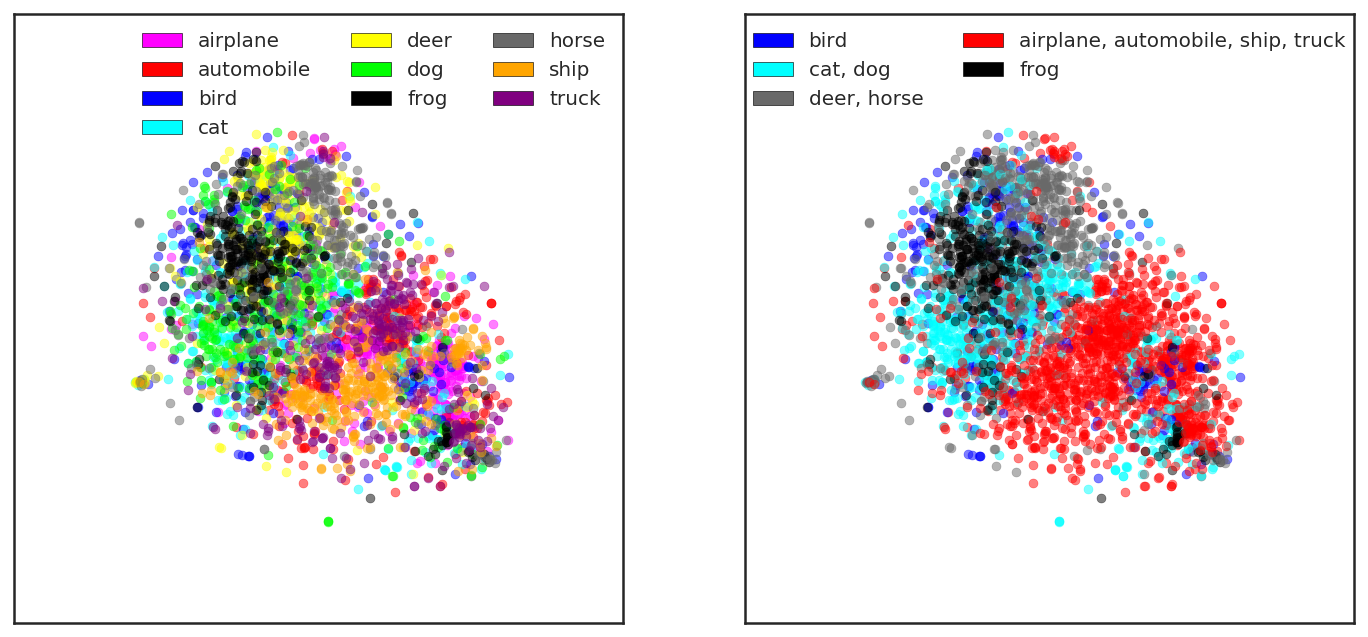
It is generally expected that images from the same class are mapped to the same region of the latent space. Fig. 7 illustrates the t-SNE (TSNE) plot of latent variables inferred from 3000 examples from the test set of CIFAR-10 colour coded based on class labels. As can also be seen on the right hand plot classes that are closest are also mostly the one that have close semantic and often visual relationships (e.g., cat and dog, or deer and horse).

Figure 7: t-SNE plot of the posterior mean for 3000 CIFAR-10 images. Note the adjacent groups and mixed regions of the plot: cats and dogs images are mostly interspersed as are automobiles and trucks.The highest concentration of horses are on top of the region right above where deer examples are.

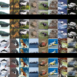
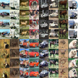
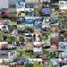
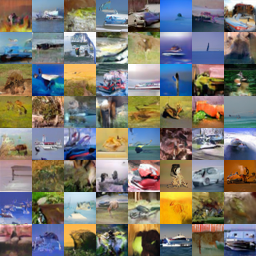
Appendix H Additional Samples

Figure 8: Additional ImageNet samples. Top left: Each column is interpolation in the latent space. Top right: ”Day dream” samples where we alternate between sampling ${\mathbf{x}}\sim p({\mathbf{x}}|{\mathbf{z}})$ and ${\mathbf{z}}\sim q({\mathbf{z}}|{\mathbf{x}})$. Bottom left: Each half-column contains in order an original image from the validation set, occlusion of that image, and two reconstructions from different posterior samples. Bottom right: Each half-column contains in order an original image from the validation set, followed by 3 reconstructions from different posterior samples.

Figure 9: Additional CIFAR-10 samples. Top left: Each column is interpolation in the latent space. Top right: ”Day dream” samples where we alternate between sampling ${\mathbf{x}}\sim p({\mathbf{x}}|{\mathbf{z}})$ and ${\mathbf{z}}\sim q({\mathbf{z}}|{\mathbf{x}})$. Bottom left: Each half-column contains in order an original image from the test set, occlusion of that image, and two reconstructions from different posterior samples. Bottom right: Each half-column contains in order an original image from the test set, followed by 3 reconstructions from different posterior samples.

Figure 10: Random samples from the auxiliary (left) and AR(1) (right) priors of our high-rate (top) and low-rate(bottom) CIFAR-10 models. The high-rate (low-rate) model has -ELBO of 2.90 (2.83) and KL of 0.10 (0.01) bits/dim. Notice that in the high rate model that has a larger value of $\alpha$, samples from the AR(1) prior can turn out too smooth compared to natural images. This is because of the gap between the prior and the marginal posterior, that is closed by the auxiliary prior.

Figure 11: Additional unconditional random samples from Imagenet 32x32. Each half-column in each block contains 4 decodings of the same sample ${\mathbf{z}}\sim p_{aux}({\mathbf{z}})$

Figure 12: One at a time interpolation of latent dimensions of a sample from the AR(1) prior. The sentences of each segment are generated by sampling a 32 element sequence of 2D random vectors from the autoregressive prior, fixing one dimension interpolating the other dimension linearly between $\mu\pm 3\sigma$.

Figure 13: One at a time interpolation of latent dimensions of a sample from the auxiliary prior. The generation procedure is identical to Fig. 12 with the exception that the initial vector is sampled from the auxiliary prior.

Figure 14: Text completion samples. For each sentence we prime the decoder with a fragment of a random sample from the validation set (shown in bold), and condition the decoder on interpolations between two samples from the latent space.

References

- Abadi et al. (2016) Martín Abadi, Paul Barham, Jianmin Chen, Zhifeng Chen, Andy Davis, Jeffrey Dean, Matthieu Devin, Sanjay Ghemawat, Geoffrey Irving, Michael Isard, Manjunath Kudlur, Josh Levenberg, Rajat Monga, Sherry Moore, Derek G. Murray, Benoit Steiner, Paul Tucker, Vijay Vasudevan, Pete Warden, Martin Wicke, Yuan Yu, and Xiaoqiang Zheng. Tensorflow: A system for large-scale machine learning. In Proceedings of the 12th USENIX Conference on Operating Systems Design and Implementation, OSDI’16, pp. 265–283, Berkeley, CA, USA, 2016. USENIX Association. ISBN 978-1-931971-33-1. URL http://dl.acm.org/citation.cfm?id=3026877.3026899.
- Alemi et al. (2017) Alexander A Alemi, Ben Poole, Ian Fischer, Joshua V Dillon, Rif A Saurous, and Kevin Murphy. Fixing a Broken ELBO. 2017. ISSN 1938-7228. URL http://arxiv.org/abs/1711.00464.
- Alemi et al. (2018) Alexander A Alemi, Ian Fischer, and Joshua V Dillon. Uncertainty in the variational information bottleneck. arXiv preprint arXiv:1807.00906, 2018.
- Ba et al. (2016) Lei Jimmy Ba, Ryan Kiros, and Geoffrey E. Hinton. Layer normalization. CoRR, abs/1607.06450, 2016.
- Babaeizadeh et al. (2017) Mohammad Babaeizadeh, Chelsea Finn, Dumitru Erhan, Roy H. Campbell, and Sergey Levine. Stochastic variational video prediction. CoRR, abs/1710.11252, 2017.
- Bowman et al. (2015) Samuel R. Bowman, Luke Vilnis, Oriol Vinyals, Andrew M. Dai, Rafal Jozefowicz, and Samy Bengio. Generating Sentences from a Continuous Space. 2015. doi: 10.18653/v1/K16-1002. URL http://arxiv.org/abs/1511.06349.
- Chelba et al. (2013) Ciprian Chelba, Tomas Mikolov, Mike Schuster, Qi Ge, Thorsten Brants, and Phillipp Koehn. One billion word benchmark for measuring progress in statistical language modeling. CoRR, abs/1312.3005, 2013.
- Chen et al. (2016) Xi Chen, Diederik P Kingma, Tim Salimans, Yan Duan, Prafulla Dhariwal, John Schulman, Ilya Sutskever, and Pieter Abbeel. Variational Lossy Autoencoder. In Iclr, pp. 1–14, nov 2016. URL http://arxiv.org/abs/1611.02731.
- Chen et al. (2017) Xi Chen, Nikhil Mishra, Mostafa Rohaninejad, and Pieter Abbeel. PixelSNAIL: An Improved Autoregressive Generative Model. pp. 12–17, 2017. URL http://arxiv.org/abs/1712.09763.
- Chung et al. (2015) Junyoung Chung, Kyle Kastner, Laurent Dinh, Kratarth Goel, Aaron Courville, and Yoshua Bengio. A Recurrent Latent Variable Model for Sequential Data. Advances in Neural Information Processing Systems 28 (NIPS 2015), pp. 8, 2015. ISSN 10495258. URL http://arxiv.org/abs/1506.02216.
- Cover & Thomas (2006) Thomas M. Cover and Joy A. Thomas. Elements of Information Theory (Wiley Series in Telecommunications and Signal Processing). Wiley-Interscience, New York, NY, USA, 2006. ISBN 0471241954.
- Davidson et al. (2018) Tim R Davidson, Luca Falorsi, Nicola De Cao, Thomas Kipf, and Jakub M Tomczak. Hyperspherical variational auto-encoders. arXiv preprint arXiv:1804.00891, 2018.
- Deng et al. (2009) J. Deng, W. Dong, R. Socher, L.-J. Li, K. Li, and L. Fei-Fei. ImageNet: A Large-Scale Hierarchical Image Database. In CVPR09, 2009.
- Denton & Fergus (2018) Emily Denton and Rob Fergus. Stochastic video generation with a learned prior. CoRR, abs/1802.07687, 2018.
- Graves & Menick (2014) Alex Graves and Jacob Menick. Associative Compression Networks for Representation Learning. 2014.
- Gregor et al. (2016) Karol Gregor, Frederic Besse, Danilo Jimenez Rezende, Ivo Danihelka, and Daan Wierstra. Towards conceptual compression. In D. D. Lee, M. Sugiyama, U. V. Luxburg, I. Guyon, and R. Garnett (eds.), Advances in Neural Information Processing Systems 29, pp. 3549–3557. Curran Associates, Inc., 2016. URL http://papers.nips.cc/paper/6542-towards-conceptual-compression.pdf.
- Gulrajani et al. (2016) Ishaan Gulrajani, Kundan Kumar, Faruk Ahmed, Adrien Ali Taiga, Francesco Visin, David Vazquez, and Aaron Courville. PixelVAE: A Latent Variable Model for Natural Images. pp. 1–9, 2016. ISSN 0066-4308. doi: 10.1146/annurev.psych.53.100901.135239. URL http://arxiv.org/abs/1611.05013.
- Guu et al. (2017) Kelvin Guu, Tatsunori B Hashimoto, Yonatan Oren, and Percy Liang. Generating Sentences by Editing Prototypes. 6:437–450, 2017. ISSN 1938-7228. URL http://arxiv.org/abs/1709.08878.
- Higgins et al. (2017) Irina Higgins, Loic Matthey, Arka Pal, Christopher Burgess, Xavier Glorot, Matthew Botvinick, Shakir Mohamed, and Alexander Lerchner. -VAE: Learning Basic Visual Concepts with a Constrained Variational Framework. In ICLR, 2017.
- Hoffman et al. (2016) Matthew D Hoffman, Matthew J Johnson, and Google Brain. ELBO surgery: yet another way to carve up the variational evidence lower bound. Advances in Approximate Bayesian Inference, NIPS Workshop, (5), 2016. URL http://approximateinference.org/accepted/HoffmanJohnson2016.pdf.
- Jimenez Rezende & Viola (2018) D. Jimenez Rezende and F. Viola. Taming VAEs. ArXiv e-prints, October 2018.
- Kim et al. (2018) Yoon Kim, Sam Wiseman, Andrew Miller, David Sontag, and Alexander Rush. Semi-amortized variational autoencoders. In Jennifer Dy and Andreas Krause (eds.), Proceedings of the 35th International Conference on Machine Learning, volume 80 of Proceedings of Machine Learning Research, pp. 2678–2687, Stockholmsmässan, Stockholm Sweden, 10–15 Jul 2018. PMLR. URL http://proceedings.mlr.press/v80/kim18e.html.
- Kingma & Ba (2014) Diederik P. Kingma and Jimmy Ba. Adam: A method for stochastic optimization. CoRR, abs/1412.6980, 2014. URL http://dblp.uni-trier.de/db/journals/corr/corr1412.html#KingmaB14.
- Kingma & Welling (2013) Diederik P. Kingma and Max Welling. Auto-encoding variational bayes. CoRR, abs/1312.6114, 2013.
- Kingma et al. (2016) Diederik P Kingma, Tim Salimans, Rafal Jozefowicz, Xi Chen, Ilya Sutskever, and Max Welling. Improving Variational Inference with Inverse Autoregressive Flow. (2011), 2016. ISSN 10495258. URL http://arxiv.org/abs/1606.04934.
- (26) Alex Krizhevsky, Vinod Nair, and Geoffrey Hinton. Cifar-10 (canadian institute for advanced research). URL http://www.cs.toronto.edu/~kriz/cifar.html.
- Larsen et al. (2016) Anders Boesen Lindbo Larsen, Søren Kaae Sønderby, Hugo Larochelle, and Ole Winther. Autoencoding beyond pixels using a learned similarity metric. In International Conference on Machine Learning, pp. 1558–1566, 2016.
- Lucas & Verbeek (2017) Thomas Lucas and Jakob Verbeek. Auxiliary guided autoregressive variational autoencoders. arXiv preprint arXiv:1711.11479, 2017.
- Ostrovski et al. (2018) Georg Ostrovski, Will Dabney, and Remi Munos. Autoregressive quantile networks for generative modeling. In Jennifer Dy and Andreas Krause (eds.), Proceedings of the 35th International Conference on Machine Learning, volume 80 of Proceedings of Machine Learning Research, pp. 3936–3945, Stockholmsmässan, Stockholm Sweden, 10–15 Jul 2018. PMLR. URL http://proceedings.mlr.press/v80/ostrovski18a.html.
- Parmar et al. (2018) Niki Parmar, Ashish Vaswani, Jakob Uszkoreit, Łukasz Kaiser, Noam Shazeer, Alexander Ku, and Dustin Tran. Image Transformer. 2018. ISSN 1938-7228. URL http://arxiv.org/abs/1802.05751.
- Rezende & Mohamed (2015) Danilo Jimenez Rezende and Shakir Mohamed. Variational inference with normalizing flows. In Proceedings of the 32Nd International Conference on International Conference on Machine Learning - Volume 37, ICML’15, pp. 1530–1538. JMLR.org, 2015. URL http://dl.acm.org/citation.cfm?id=3045118.3045281.
- Rezende et al. (2014) Danilo Jimenez Rezende, Shakir Mohamed, and Daan Wierstra. Stochastic Backpropagation and Approximate Inference in Deep Generative Models. 32, 2014. ISSN 10495258. doi: 10.1051/0004-6361/201527329. URL http://arxiv.org/abs/1401.4082.
- Roy et al. (2018) Aurko Roy, Ashish Vaswani, Arvind Neelakantan, and Niki Parmar. Theory and experiments on vector quantized autoencoders. arXiv preprint arXiv:1805.11063, 2018.
- Salimans et al. (2017) Tim Salimans, Andrej Karpathy, Xi Chen, and Diederik P Kingma. PixelCNN++: Improving the PixelCNN with Discretized Logistic Mixture Likelihood and Other Modifications. pp. 1–9, 2017. ISSN 9781467324755. URL http://arxiv.org/abs/1701.05517.
- Tomczak & Welling (2017) Jakub M. Tomczak and Max Welling. VAE with a vampprior. CoRR, abs/1705.07120, 2017. URL http://arxiv.org/abs/1705.07120.
- Turner & Sahani (2007) R. E. Turner and M. Sahani. A maximum-likelihood interpretation for slow feature analysis. Neural Computation, 19(4):1022–1038, 2007. ISSN 0899-7667. doi: http://dx.doi.org/10.1162/neco.2007.19.4.1022.
- van den Oord et al. (2016a) Aäron van den Oord, Nal Kalchbrenner, and Koray Kavukcuoglu. Pixel recurrent neural networks. CoRR, abs/1601.06759, 2016a. URL http://arxiv.org/abs/1601.06759.
- van den Oord et al. (2016b) Aaron van den Oord, Nal Kalchbrenner, and Koray Kavukcuoglu. Pixel Recurrent Neural Networks. In International Conference on Machine Learning, volume 48, pp. 1747–1756, 2016b. ISBN 9781510829008. URL http://arxiv.org/abs/1601.06759.
- van den Oord et al. (2017) Aäron van den Oord, Oriol Vinyals, and Koray Kavukcuoglu. Neural discrete representation learning. CoRR, abs/1711.00937, 2017. URL http://arxiv.org/abs/1711.00937.
- van der Maaten & Hinton (2008) L.J.P. van der Maaten and G.E. Hinton. Visualizing high-dimensional data using t-sne. 2008.
- Vaswani et al. (2017) Ashish Vaswani, Noam Shazeer, Niki Parmar, Jakob Uszkoreit, Llion Jones, Aidan N. Gomez, Lukasz Kaiser, and Illia Polosukhin. Attention Is All You Need. (Nips), 2017. ISSN 0140-525X. doi: 10.1017/S0140525X16001837. URL http://arxiv.org/abs/1706.03762.
- Vaswani et al. (2018) Ashish Vaswani, Samy Bengio, Eugene Brevdo, François Chollet, Aidan N. Gomez, Stephan Gouws, Llion Jones, Lukasz Kaiser, Nal Kalchbrenner, Niki Parmar, Ryan Sepassi, Noam Shazeer, and Jakob Uszkoreit. Tensor2tensor for neural machine translation. CoRR, abs/1803.07416, 2018.
- Wiskott & Sejnowski (2002) Laurenz Wiskott and Terrence J. Sejnowski. Slow feature analysis: Unsupervised learning of invariances. Neural Comput., 14(4):715–770, April 2002. ISSN 0899-7667. doi: 10.1162/089976602317318938. URL http://dx.doi.org/10.1162/089976602317318938.
- Xu & Durrett (2018) Jiacheng Xu and Greg Durrett. Spherical latent spaces for stable variational autoencoders. Proc. Empirical Methods in Natural Language Processing, 2018.
- Yang et al. (2017) Zichao Yang, Zhiting Hu, Ruslan Salakhutdinov, and Taylor Berg-Kirkpatrick. Improved Variational Autoencoders for Text Modeling using Dilated Convolutions. 2017. URL http://arxiv.org/abs/1702.08139.
- Zhao et al. (2017) Shengjia Zhao, Jiaming Song, and Stefano Ermon. InfoVAE: Balancing Learning and Inference in Variational Autoencoders. ICML Workshop, 2017. URL http://arxiv.org/abs/1706.02262.