Supplementary material for paper submission #6103
Detecting Overfitting of Deep Generative Networks via Latent Recovery
Abstract
This document gives additional details and experiments regarding:
-
•
results on MNIST and CIFAR-10 datasets (Section 1),
-
•
study of local overfitting (Section 2),
-
•
visual results of recovery with various objective loss functions (Section 3),
-
•
failure cases and success rate of recovery (Section 4),
-
•
convergence study of the latent recovery optimization (Section 5).
1 Additional Results on other Datasets (MNIST & CIFAR-10)
We compute the MRE-gap and KS statistic on a few datasets in Table 1. We note the results are consistent with the results those in Table 1 in the paper. In particular, memorization is not detectable in glo and cgan models when enough data is used.
| KS p-value | MRE-gap | MRE | ||||
| train vs val | train | val | generated | |||
| MNIST | dcgan | 2.41e-01 | 8.85e-02 | 3.00e-02 | 2.75e-02 | 6.89e-03 |
| glo-1024 | \cellcolormyblue0.00e+00 | \cellcolormygreen6.78e-01 | 2.86e-04 | 8.88e-04 | 1.49e-03 | |
| glo-16384 | 3.48e-01 | 6.45e-03 | 8.72e-04 | 8.77e-04 | 1.41e-03 | |
| cgan-16384 | 7.43e-02 | 2.29e-02 | 4.56e-02 | 4.67e-02 | N/A | |
| CIFAR10 | dcgan | 5.40e-01 | 3.65e-03 | 2.29e-01 | 2.28e-01 | 1.30e-03 |
| glo-1024 | \cellcolormyblue0.00e+00 | \cellcolormygreen5.84e-01 | 2.77e-03 | 6.67e-03 | 8.53e-04 | |
| glo-16384 | 3.48e-01 | 6.45e-03 | 8.72e-04 | 8.77e-04 | 1.41e-03 | |
2 Local vs Global overfitting
While GANs geneartors appear to not overfit the training set on the entire image, one may wonder if they do however overfit training image patches. To investigate this, we take of Eq. to be a masking operator on eye and mouth regions of the image. To first verify this optimization is stable (see Section 5, for more information of stability of optimization), we recover eyes pggan for a number of random initializations in Fig. 1. Finally, we observe the recovery histograms and KS p-values for patches in Fig. 2.

Target images (after cropping eye on training images)
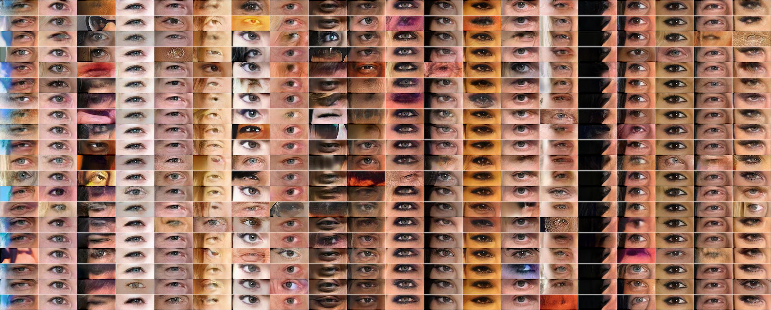
Recovered images (for different initialization)


3 Comparison with Other Loss Functions
We visually compare in Fig. 3 the simple Euclidean loss used in this paper for analyzing overfitting (i.e. in Eq. ) with other operators:
-
•
pooling by a factor of 32 (as used in applications for super-resolution);
-
•
various convolutional layers of the VGG-19 (i.e. the perceptual loss previously mentioned in the paper).
While the perceptual loss has been shown to be effective for many synthesis tasks, it appears to hinder optimization in the case when interacting with a high quality generator .
|
Targets |
|
|
|
pool |
|
VGG-19 |
|
|
|
pool |
|
VGG-19 |

4 Optimization Failures
We noted that most networks had the ability to exactly recover generated images. This is shown in Fig. 4, with failure cases highlighted in red. Interestingly, some networks were not able to recover their generated images at all, for example Fig. 4 was a PGGAN trained on LSUN Bedroom, which did not verbatim recover any image. We think this may suggest a more complex latent space for some networks trained on LSUN, with many local minima to equation . Because we assert that we are finding the nearest neighbors in the space of generated images, we did not analyze networks which could not recover generated images. It should be noted that some LSUN networks did recover generated images however.

![[Uncaptioned image]](/html/1901.03396/assets/fig_gen_recov/app_pggbed_gen_fail.jpg)
Generated recovery for PGGAN on LSUN Bedroom. Recovery failure detection with thresholding. First row generated images and second row is recoveries.
4.1 Recovery Success Rate
Disregarding networks which could not recover generated images, some networks had higher failure rates than others. To determine failure cases numerically, we chose a recovery error threshold of to signify a plausible recovery for real images (for generated images a much smaller threshold of can be used). Table 2 summarizes recovery rates for a few networks. The MESCH resnets were notably less consistent than other architectures. To study if these failures were due to bad initialization, we tried simply restarting optimization 10 times per image, and saw the success rate go from 68% to 98% shown in Table 2 as MESCH-10-RESTART. This shows that likely all training and generated images can be recovered decently well with enough restarts.
| train | test | generated | |
| MESCH | 68% | 67% | 67% |
| MESCH-10-RESTART | 98% | 99% | 96% |
| DC-CONV | 82% | 82% | 100% |
| PGGAN | 97% | 96% | 95% |
5 Convergence analysis of latent recovery
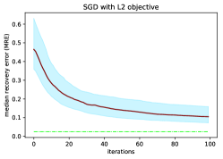
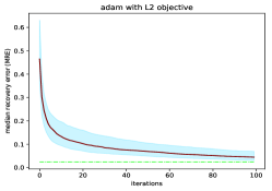
In general, optimization was successful and converges nicely for most random initializations. We provide numerical and visual evidence in this section supporting fast and consistent convergence of LBFGS compared to other optimization techniques like SGD or Adam.
5.1 Protocol
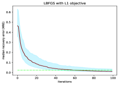
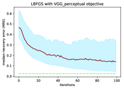
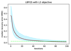
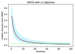
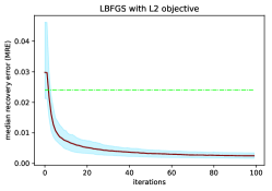
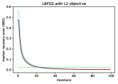
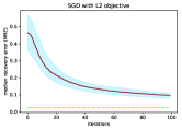
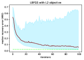
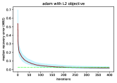
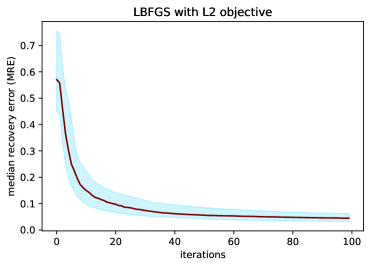
To demonstrate that the proposed optimization of the latent recovery is stable enough to detect overfitting, the same protocol is repeated in the following experiments. We used the same 20 random latent codes to generate images as target for recovery: . We also used 20 real images as targets the same as in Section 2 for local recovery. We also initialized the various optimization algorithms with the same 20 random latent codes . We plot the median recovery error (MRE) for 100 iterations. This curve (in red) is the median of all MSE curves (whatever the objective function is) and is compared to the 25th and 75th percentile (in blue) of those 400 curves.
5.2 Comparison of optimization algorithm
We first show the average behavior in Fig. 6 the chosen optimization algorithm (LBFGS) to demonstrate that it convergences much faster than SGD and Adam. A green dashed line shows the threshold used to detect if the actual nearest neighbor is well enough recovered (). One can see that only 50 iterations are required in half the case to recover the target image.
| Target images (generated with PGGAN) | |
|
Initialization (LBFGS)
|
|
|
Initialization (SGD)
|
 |
 |
 |
| LBFGS | SGD | Adam |
5.3 Comparison of objective loss functions
In Figure 7 are plotted the MRE (median recovery error) when optimizing various objective functions:
-
•
Euclidean distance () as used throughout the paper,
-
•
Manhattan distance (), which is often used as an alternative to the Euclidean distance that is more robust to outliers,
-
•
VGG-based perceptual loss.
 |
 |
 |
| Euclidean distance () | Manhattan distance () | Perceptual loss (VGG-19) |
5.4 Convergence with operator
Figure 8 demonstrates convergence under various operators .
 |
 |
 |
| (resolution of 1024) | (resolution of 128) | (cropping around mouth area) |
5.5 Recovery with other generators
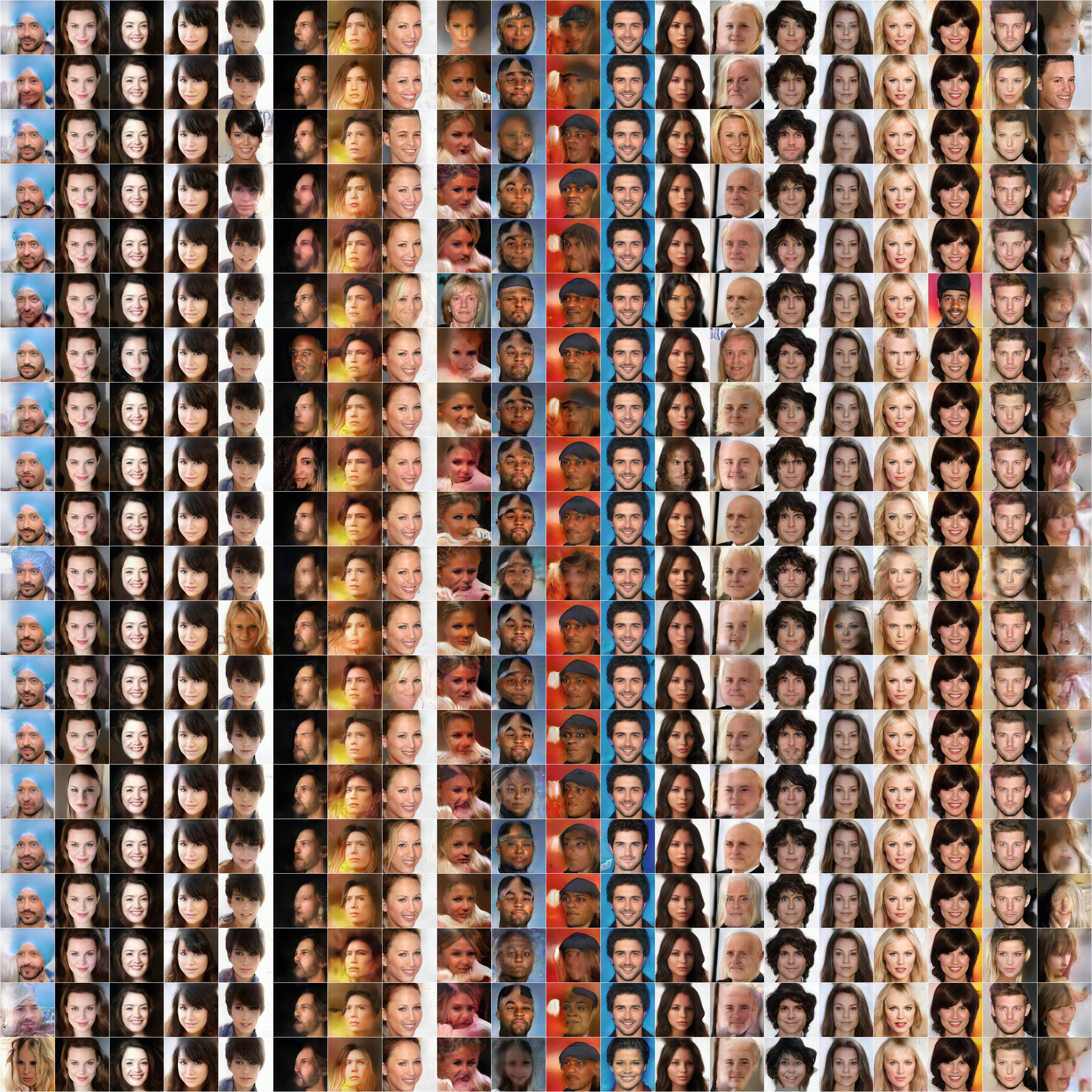
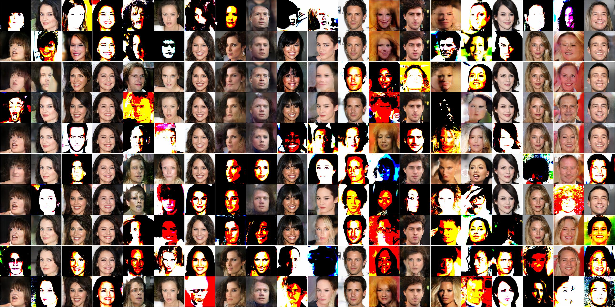
Figure 9 displays median recovery error (MRE) when optimizing with LBFGS and SGD for DCGAN and MESCH generators. Visual results are given for LBFGS in Figures 11 and 12. The MESCH network is more inconsistent, but using 10 random initialization is enough to ensure the recovery of a generated (or real) image with 96% chance.
 |
 |
 |
 |
| DCGAN with LBFGS | DCGAN with SGD | MESCH with LBFGS | MESCH with Adam (400 iterations) |
5.6 Convergence on real images
Figure 10 shows highly consistent recover on real images for the PGGAN network.
| Target images (from the training set) | |
|
Initialization
|
 |
| Target images (generated with DCGAN) | |
|
Initialization
|
| Target images (generated with MESCH) | |
|
Initialization
|
 |