Modified Jaccard Index Analysis and Adaptive Feature Selection for Location Fingerprinting with Limited Computational Complexity

Abstract

We propose an approach for fingerprinting-based positioning which reduces the data requirements and computational complexity of the online positioning stage. It is based on a segmentation of the entire region of interest into subregions, identification of candidate subregions during the online-stage, and position estimation using a preselected subset of relevant features. The subregion selection uses a modified Jaccard index which quantifies the similarity between the features observed by the user and those available within the reference fingerprint map. The adaptive feature selection is achieved using an adaptive forward-backward greedy search which determines a subset of features for each subregion, relevant with respect to a given fingerprinting-based positioning method. In an empirical study using signals of opportunity for fingerprinting the proposed subregion and feature selection reduce the processing time during the online-stage by a factor of about 10 while the positioning accuracy does not deteriorate significantly. In fact, in one of the two study cases the $\mathrm{90^{th}}$ percentile of the circular error increased by 7.5% while in the other study case we even found a reduction of the corresponding circular error by 30%.

1 Introduction

Fingerprinting-based indoor positioning systems (FIPSs) are attractive for providing location of users or mobile assets because they can exploit signals of opportunity (SoP) and infrastructure already existing for other purposes (He and Chan 2016). They require no or little extra hardware, (He and Chan 2016), and differ in that respect from many other approaches to indoor positioning like e.g., the ones using infrared beacons (Lee et al. 2004), ultrasonic signals (Hazas and Hopper 2006), Bluetooth low energy (BLE) beacons (Kalbandhe and Patil 2016), radio frequency identification (RFID) tags (Bekkali et al. 2007), ultra wideband (UWB) signals (Ingram et al. 2004), or foot-mounted inertial measurement units (IMUs) (Gu et al. 2017). FIPS benefit from the spatial variability of a wide variety of observable features or signals like received signal strength (RSS) from wireless local area network (WLAN) access points (APs) (Padmanabhan et al. 2000; Youssef and Agrawala 2008; Torres-Sospedra et al. 2014; Jun et al. 2017; Mendoza-Silva et al. 2018), magnetic field strengths (Saxena and Zawodniok 2014; Torres-Sospedra et al. 2015; Xie et al. 2016), or RSS of cellular towers (Driusso et al. 2016). Such signals are location dependent features, many of which can easily be measured using a variety of mobile devices (e.g., smart phones or tablets). FIPSs are therefore also called feature-based indoor positioning systems (Kasprzak et al. 2013). The attainable quality of the position estimation using FIPS mainly depends on the spatial gradient of the features and on their stability or predictability over time (Niedermayr et al. 2014).

Key challenges of FIPS, especially the ones using RSS readings from WLAN APs, are discussed e.g., in (Kushki et al. 2007) and more recently in (He and Chan 2016; Yassin et al. 2017). The former publication focuses on four challenges of FIPS utilizing vectors of RSS from WLAN AP as features. In particular, the paper addresses i) the generation of a fingerprint database to provide a reference fingerprint map (RFM) for positioning, ii) pre-processing of fingerprints for reducing computational complexity and enhancing accuracy, iii) selection of APs for positioning, and iv) estimation of the distance between a fingerprint measured by the user and the fingerprints represented within in the reference database. Extensions to large indoor regions and handling of variations of observable features caused by the changes of indoor environments or signal sources of the features (e.g., replacement of broken APs) are addressed in (He and Chan 2016).

Regarding generation of the RFM, various approaches have been proposed (He and Chan 2016). Initially, the features were mapped by dedicated surveying measurements (e.g., (Youssef and Agrawala 2008; Park et al. 2010)). The resulting RFMs were accurate at the time of acquisition. However, such measurements are labor-intensive and time-consuming. Approaches based on forward modeling, e.g., using indoor propagation models (Jung et al. 2011; El-Kafrawy et al. 2010; Bisio et al. 2014) or ray tracing (Renaudin et al. 2018), were proposed as a cost-effective alternative, especially in case of radio frequency signal strengths as features. However, the accuracy of the resulting RFM depends on the validity of the model assumptions including the wave propagation models, the geometry and material properties of the objects and structures in the indoor space, and the location and antenna gain patterns of the signal sources. For many real-world application scenarios it is thus typically lower than the accuracy of measurement-based RFM generation. More recently, approaches for RFM generation using the sensors built into the mobile user devices have been proposed. They can be differentiated according to the degree of user participation. Data collection for RFM generation can be done by an application running in the background such that the user only needs to consent to contributing data but not actively participate otherwise. Other approaches require the user to manually indicate his/her location on a map or to signal to the application that the current location corresponds to a certain marked ground truth, see e.g. (Wu et al. 2013; Ledlie et al. 2011; Li et al. 2013). For refining the RFM various approaches have been proposed, e.g., interpolation/extrapolation (Talvitie et al. 2015; Sorour et al. 2015) or kernel-smoothing (Huang and Manh 2016). We are not focusing on reducing the workload for building the RFM. However, we validate the proposed approach using a kinematically collected RFM (see Section 4) which is similar to a standard survey but less time-consuming.

The contribution of this paper is to reduce the online positioning computation complexity by introducing a specific approach to subregion selection and feature selection into the online positioning process. The proposed approach includes machine learning algorithms, i.e. algorithms whose performance on the specific task improves with experience (Mitchell 1997) and which are thus suitable for fingerprinting-based positioning (Bishop 2006). It is applicable to FIPSs using opportunistically measured location-relevant features. In case of FIPSs using SoP, the difficulty lies in both the type and number of features varying across the region of interest. This introduces a critical limitation which prevents the applicability of the aforementioned FIPS solutions due to changes of the dimension of the feature space across time and across location coordinate space. For instance, the fingerprinting-based positioning methods including the typical ones, e.g., $k$-nearest neighbors ($k$NN) (Padmanabhan et al. 2000) and maximum a posteriori (MAP) (Youssef and Agrawala 2008), and the advanced ones, e.g., fingerprinting-based positioning using support vector machine (SVM) (Wu et al. 2004), linear discriminant analysis (LDA) (Nuño-Barrau and Páez-Borrallo 2006), Bayesian network (Nandakumar et al. 2012), and Gaussian process (Ouyang et al. 2012), cannot be applied without special precautions for handling the varying dimension in such cases. Few previous publications address handling this problem e.g., (Zhou and Wieser 2018a). Additionally, the computational complexity of these fingerprinting-based positioning methods is proportional to the number of reference locations in the RFM and the number of observable features. This makes these approaches computationally expensive in large RoIs with many reference locations and many available features unless introducing specific means for mitigation. The discrepancy of the feature dimension and the computational complexity problems is typically mitigated by introducing subregion selection and feature selection (Zhou and Wieser 2018b; Kushki et al. 2007; Feng et al. 2012; Ouyang et al. 2012; Khalajmehrabadi et al. 2017).

In this paper we propose (i) subregion selection based on a modified Jaccard index (MJI), (ii) a forward-greedy search to find an appropriate number of subregions, and (iii) an adaptive forward-backward greedy search (AFBGS) algorithm (Zhang 2011) for selecting the relevant features for each subregion. We demonstrate the application of the proposed algorithms to both MAP- and kNN-based position estimation. We finally validate the performance of the proposed approach by carrying out experiments in two RoIs of different size using two types of opportunistically measured signals (i.e., WLAN and BLE).

The structure of the paper is as follows: A short review of the previous publications addressing the approaches for subregion selection and feature selection is given in Section 2. In Section 3, the MJI-based subregion selection, AFBGS-based feature selection, and the modified online positioning process are presented along with the computational complexity. We illustrate and validate the performance of the proposed approach in Section 4 by applying it to an FIPS, which utilizes SoP as the location-relevant features, and we compare the results to those obtained using previously proposed methods.

Table 1: Selected acronyms used herein

Acronym	Meaning
FIPS	fingerprinting-based indoor positioning system
RSS	received signal strength
SoP	signals of opportunity
RFM	reference fingerprint map
$k$NN	$k$ nearest neighbors
MAP	maximum a posteriori
MJI	modified Jaccard index
AFBGS	adaptive forward-backward greedy search
LASSO	least absolute shrinkage and selection operator
MSE	mean squared error
ECDF	empirical cumulative distribution function

2 Related work

2.1 Subregion selection

The subregion selection process contributes to constraining the search space. The selected subregions are treated as coarse approximations of the user’s location. The process of refining the coordinate estimates is then carried out only within these subregions and the search space for the final estimate is thus independent of the size of the RoI. There are mainly two types of approaches for subregion selection: approaches based on clustering and approaches based on similarity metrics. (Feng et al. 2012; Karegar 2017), and (Chen et al. 2006; Ouyang et al. 2012) applied affinity propagation and $k$-means clustering to divide the RoI into a given number of subregions according to the features collected within the RoI. Both papers present clustering-based subregion selection, and require prior definition of the desired number of subregions and knowledge of all features observable within the entire RoI. These clustering-based approaches take the fingerprint measured by the user into account during the clustering process which thus has to be repeated with each new user fingerprint obtained.

Similarity metric-based subregion selection relies on the identification of the subregions whose fingerprints contained in the RFM are most similar to the fingerprint observed by the user. They differ depending on the chosen similarity metric. E.g., (Kushki et al. 2007) use the Hamming distance for this purpose, measuring only the difference in terms of observability of the features, not their actual values. Still, these approaches typically need prior information on all observable features within the entire RoI when associating a user observed features with a subregion. This may be a severe limitation in case of a large RoI or changes of availability of the features. MJI-based subregion selection as proposed in this paper belongs to similarity metric-based subregion selection. However, the approach proposed herein requires only the prior knowledge of the features observable within each subregion when quantifying the similarity metric between the observations in the RFM and in the user observed measurements.

2.2 Selection of relevant features

Approaches to selection of features (or sparse representation) actually used for positioning differ w.r.t. several perspectives. We focus on three aspects in their review: i) whether they take the relationship between positioning accuracy and selected features into account, ii) whether they help to reduce the computational complexity of position estimation, and iii) whether they are applicable to a variety of features or only features of a certain type. The chosen features for positioning should be the ones allowing to achieve the best positioning accuracy using the specific fingerprinting-based positioning method or achieving a useful compromise between accuracy and reduced computational burden.

Previous publications focused on feature selection for FIPS using RSS from WLAN APs and consequently addressed the specific problem of AP selection rather than the more general feature selection. (Chen et al. 2006) and (Feng et al. 2012) proposed using the subsets of APs whose RSS readings are the strongest assuming that the strongest signals provide the highest probability of coverage over time and the highest accuracy. (Kushki et al. 2007) and (Chen et al. 2006) applied a divergence metric (Bhattacharyya distance and information gain, respectively) to minimize the redundancy and maximize the information gained from the selected APs. The limitations of these approaches are: i) they are only applicable to the FIPS based on RSS from WLAN APs, and ii) they only take the values of the features into account as selection criteria instead of the actual positioning accuracy. (Kushki et al. 2010) proposed an AP selection strategy able to choose APs ensuring a certain positioning accuracy using a nonparametric information filter. However, this approach uses consecutively measured fingerprints to select the subset of APs maximizing the discriminative ability w.r.t. localization. This method therefore needs several online observations for estimating one current position.

In (Zhou and Wieser 2018b), a feature selection algorithm based on randomized LASSO (Tibshirani 1996), an $L_{1}$-regularized linear regression model, for selecting the relevant features for positioning is proposed. Each feature within the subregion is associated with an estimated coefficient. If the coefficient is sufficiently different from zero the corresponding feature is identified as relevant. However, this approach only connects the feature selection with the positioning error indirectly. Furthermore, LASSO-based feature selection is equivalent to MAP if the likelihood is Gaussian and the prior distribution is Laplace (Park and Casella 2008). These two assumptions are not necessarily justified with fingerprinting-based positioning. It is difficult to find a proper value of the hyper-parameter of LASSO-based feature selection, which makes the feature selection unstable (Fastrich et al. 2015). Finally, this feature selection algorithm is prone to overfitting. Applying this approach to select the relevant features for each subregion requires the number of observations in each subregion to be much larger than the number of the dimension of the features (e.g., the number of observable WLAN APs or BLE beacons). Normally, this requirement is not met in case of fingerprinting-based positioning using SoPs as the features.

In this paper, we thus propose an approach based on AFBGS to choose the most relevant features for fingerprinting-based positioning. This method differs from the previously mentioned ones in three ways: i) it takes the positioning error into account directly, i.e. the feature selecting process is directly combined with the fingerprinting-based positioning methods that are used at the online stage, ii) wrongly selected features from the forward greedy search step can be adaptively corrected by a backward greedy search step (Zhang 2011), and iii) it is a data-driven algorithm adapting automatically to the number of observations of each subregion.

3 The proposed approach

In this section, we briefly summarize the fundamentals of fingerprinting-based positioning and present the main contributions of this paper to reduce the computational complexity independent of the size of the RoI. In particular we present i) candidate subregion selection according to MJI, ii) selection of relevant features using AFBGS, and iii) adaptations of MAP and $k$NN-based positioning with the combination of the previous two steps. Finally we briefly discuss the computational complexity of the proposed method.

3.1 Problem formulation

Each measured feature has a unique identifier and a measured value, e.g., the measurement related to a specific WiFi AP can be identified by the media access control (MAC) address and has a RSS. It is thus formulated as a pair $(a,v)$ of attribute $a$ and value $v$. A complete measurement (i.e. fingerprint) $\mathbbm{O}_{i}^{\mathrm{u}}$ taken by user $\mathrm{u}$ at location/time $i$ consists of a set of attribute-value pairs, i.e. $\mathbbm{O}_{i}^{\mathrm{u}}:=\{(a_{ik}^{\mathrm{u}},v_{ik}^{\mathrm{u}})|a_{ik}^{\mathrm{u}}\in\mathbbm{A};v_{ik}^{\mathrm{u}}\in\varmathbb{R};k\in\{1,2,\cdots,N_{i}^{\mathrm{u}}\}\}$, where $\mathbbm{A}$ is the complete set of the identifiers of all available features and $N_{i}^{\mathrm{u}}$ ($N_{i}^{\mathrm{u}}=|\mathbbm{O}_{i}^{\mathrm{u}}|$) is the number of features observed by $\mathrm{u}$ at $i$. The set of keys of such a fingerprint is defined as $\mathbbm{A}_{i}^{\mathrm{u}}:=\{a_{ik}^{\mathrm{u}}|\exists(a_{ik}^{\mathrm{u}},v_{ik})\in\mathbbm{O}_{i}^{\mathrm{u}}\}$. A discrete RFM $\mathbbm{M}:=\{(\mathbf{l}_{j},\mathbbm{\tilde{O}}_{j}^{\mathrm{}})|\mathbf{l}_{j}\in\mathbbm{G},j\in\{1,2,\cdots,|\mathbbm{M}|\}\}$ is given as a set of position-fingerprint pairs representing the relationship between the location $\mathbf{l}$ and the features $\mathbbm{O}$ at different locations within the RoI $\mathbbm{G}$.

Specifically for the subregion selection, $\mathbbm{G}$ is divided into $M$ non-overlapping subregions of arbitrary shape, i.e. $\mathbbm{G}=\underset{i=1:M}{\cup}\,\mathbbm{g}_{i},\,\mathbbm{g}_{i}\cap\mathbbm{g}_{j}=\emptyset|i\neq j$. This segmentation can take contextual information into account by defining the subregions such that one subregion lies only in e.g. one building, one floor, one room or one corridor. Thus the concept is directly applicable to multi-building or mutli-floor situations. Each of the measurements (elements) of $\mathbbm{M}$ is assigned to the corresponding subregion. The subset of $\mathbbm{M}$ corresponding to the $g^{\mathrm{th}}$ subregion can thus be defined as $\mathbbm{M}_{g}^{\mathrm{}}:=\{(\mathbf{l}_{j},\mathbbm{\tilde{O}}_{j}^{\mathrm{}})|\mathbf{l}_{j}\in\mathbbm{g}_{g}^{\mathrm{}},j\in\{1,2,\cdots,|\mathbbm{M}_{g}^{\mathrm{}}|\}\},\mathbbm{M}_{g}^{\mathrm{}}\subseteq\mathbbm{M}$, and the set of observable features in the corresponding subregion is denoted as $\mathbbm{A}_{g}^{\mathrm{}}:=\{a|a\in\underset{j=1:|\mathbbm{M}_{g}^{\mathrm{}}|}{\cup}{\mathbbm{\tilde{A}}_{j}^{\mathrm{}}},\mathbbm{\tilde{A}}_{j}^{\mathrm{\,}}\text{ of }\mathbbm{\tilde{O}}_{j}^{\mathrm{}},\exists(\mathbf{l}_{j},\mathbbm{\tilde{O}}_{j}^{\mathrm{}})\in\mathbbm{M}_{g}^{\mathrm{}}\}(g\in\{1,2,\cdots,M\}),\mathbbm{A}_{g}^{\mathrm{}}\subseteq\mathbbm{A}$.

The positioning process consists of inferring the estimated user location $\mathbf{\hat{l}}_{i}^{\mathrm{u}}=\mathpzc{f}(\mathbbm{O}_{i}^{\mathrm{u}})$ as a function of the fingerprint and the RFM where $\mathpzc{f}$ is a suitable mapping from fingerprint to location, i.e. $\mathpzc{f}:\mathbbm{O}_{i}^{\mathrm{u}}\mapsto\mathbf{\hat{l}}_{i}^{\mathrm{u}}$. Herein we propose the following solutions for mitigating the computational load associated with the online stage:

• identifying (during the offline stage) the most relevant features within each subregion using the AFBGS such that the actual location calculation can be carried out during the online stage using only those instead of using all features;

• selecting the subregion as a coarse approximation of the actual user location based on MJI during the online-stage;

Within this paper we combine the above two steps with a MAP and $k$NN-based positioning for performance analysis. We implement it in a way to keep the computational complexity of the online stage almost independent of the size of the RoI and of the total number of observable features within the RoI.

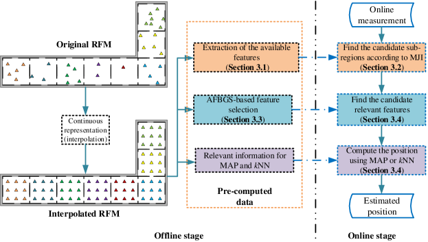
Figure 1: The proposed framework. In order to make the number of reference points within all subregions equal we interpolate the reference data in the original RFM using kernel smoothing (Berlinet and Thomas-Agnan 2011) to provide a denser regular grid of reference points. This interpolated RFM is used to calculate the pre-computed data for online positioning.

3.2 Subregion selection using MJI

MJI, an indicator of similarity between the keys of the measured fingerprints and the keys associated with the individual subregions in the RFM, is applied to identify a set of candidate subregions most probably containing the actual user location (Zhou and Wieser 2018b; Jani et al. 2015). We depict four qualitative examples in Figure 2. If the overlap between the features within a subregion (according to the RFM) and the features within a user’s observation is large, the value of the MJI is high, otherwise it is low. For a more detailed discussion of MJI see (Zhou and Wieser 2018b).

(a) High MJI value

(b) High MJI value

(c) Low MJI value

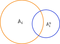
(d) Low MJI value

Figure 2: Qualitative examples of MJI values: (a) a few features within the current subset of the RFM are not measured, (b) there are some measured features which are not in the current subset of the RFM, (c) the measured features are only few of the ones in the current subset of the RFM, (d) there is little overlap between the measured features and the ones in the current subset of the RFM.

The $m$ subregions with the highest values of the MJI are selected as candidate subregions for the subsequent positioning. Their cell indices are collected in the vector $\mathbf{s}^{\mathrm{u}}_{m}\in\mathbb{N}^{m}$ for further processing. If the subregions are non-overlapping, as introduced above, $m$ needs to be large enough to accommodate situations where the actual user location is close to the border between subregions and small enough to reduce the computational burden of the subsequent user location estimation.

In order to determine a proper value of $m$, an indicator is introduced for denoting whether a validation example is contained in the selected top $m$ subregions (indicator 1) or not (indicator 0). Throughout this paper we assume that the user is actually within the RoI and thus within one subregion when the subregion selection process is carried out. Given $M^{\mathrm{val}}$ validation examples $\{(\mathbbm{O}_{n}^{\mathrm{val}},\mathbf{l}_{n}^{\mathrm{val}})\}_{n=1}^{M^{\mathrm{val}}}$, the indicator for the $n$-th example is thus defined as:

$$I(\mathbf{l}_{n}^{\mathrm{val}},m)=\Bigg{\{}\begin{array}[]{ll}1,&\mathrm{if\,\,}\mathbf{l}_{n}^{\mathrm{val}}\in\underset{j\in\mathbbm{S}^{\mathbf{l}_{n}^{\mathrm{val}}}_{m}}{\cup}\mathbbm{g}_{j}^{\mathrm{}}\\ 0,&\mathrm{otherwise}\end{array}$$ (1)

where $\mathbbm{S}^{\mathbf{l}_{n}^{\mathrm{val}}}_{m}$ contains the indices of the selected subregions for this particular validation example. The subregion selection loss is then defined as the fraction of the validation examples for which the true location is not within the selected subregions, i.e.

$$\mathpzc{L}^{\mathrm{MJI}}(m)=1-\frac{\sum_{n=1}^{M^{\mathrm{val}}}I(\mathbf{l}_{n}^{\mathrm{val}},m)}{M^{\mathrm{val}}}.$$ (2)

The subregion selection loss reduces as $m$ increases. However, increasing the number of selected subregions contradicts to the idea of reducing the computational complexity of the online positioning. Balancing between subregion selection loss and computational complexity is a multi-objective optimization problem, and it has no single optimum. Herein we decided to select an appropriate number of subregions heuristically by analyzing plots of selection loss versus $m$ and choosing a value from which on the curve is flat. I.e., at which further increasing $m$ hardly reduces the loss.

3.3 Feature selection using AFBGS

In a real-world environment there may be a large number of features available for positioning, e.g., hundreds of APs may be visible to the mobile user device in certain locations. Not all of them will be necessary to estimate the user location. In fact using only a well selected subset of the available signals instead of all will reduce the computational burden and may provide a more accurate estimate because the measured signals are affected by noise and possibly interference. Furthermore the number of observable features typically varies across the RoI e.g., due to WLAN APs antenna gain patterns, structure and furniture of the building. However, it is preferable to use the same number of features throughout the candidate subregions for assessing the similarity between the measured fingerprint and the ones extracted from the RFM during the online phase.

We therefore recommend selecting a number $h$ of features per candidate subregion for the final position estimation. To facilitate this selection during the online phase, the relevant features within each subregion are already identified beforehand once the RFM is available. We use the AFBGS (Zhang 2011) for this step. During the online phase $h$ relevant features (possibly different for each subregion) are selected among the identified ones such that they are available both within the RFM and the user fingerprint.

The combination of forward and backward steps within the algorithm makes AFBGS capable of correcting intermediate erroneous selection of features. We first shortly review both forward and backward greedy algorithms, then present AFBGS.

Let $\mathbbm{F}_{(h_{i})}$ denote the set of indices of the selected relevant features of the $i^{\mathrm{th}}$ subregion. A fingerprinting-based positioning method $\mathpzc{f}$ thus only uses these selected features to estimate the position, i.e. $\mathpzc{f}:\mathbbm{O}|\mathbbm{F}_{(h_{i})}\rightarrow\mathbf{l}$. The forward greedy search algorithm adds features one at a time picking the one causing the biggest reduction of a given loss at each step. Herein we use the mean squared error (MSE), a widely applied loss function for regression problems, as the loss metric for the feature selection. For instance, with $\mathbbm{F}_{(h_{i})}$ being the set of $h$ features selected for the $i^{\mathrm{th}}$ subregion, the loss is the MSE of the positions estimated for all validation examples using this particular set of subregions:

$$\mathpzc{L}^{\mathrm{FS}}(\mathbbm{F}_{(h_{i})})=\frac{1}{M^{\mathrm{val}}}\sum_{n=1}^{M^{\mathrm{val}}}\|\mathpzc{f}(\mathbbm{O}_{n}^{\mathrm{val}}|\mathbbm{F}_{(h_{i})})-\mathbf{l}_{n}^{\mathrm{val}}\|_{2}^{2}$$ (3)

An example of applying the forward greedy search to select features for the $i^{\mathrm{th}}$ subregion is described in Table 2. This algorithm works well in case the features are independent of each other. Otherwise the forward greedy search might wrongly select non-relevant features. Such wrong selections cannot be corrected by the forward greedy algorithm anymore. One remedy introduced to solve this problem is the backward greedy search (Table 3), which starts with all features and greedily removes them one at a time picking the one associated with the smallest increase of the loss at each step. However, also the backward greedy search has two disadvantages: i) it is computationally costly because it starts with all features; ii) it is prone to overfitting if the number of observations in each subregion is much lower than the number of observable features.

A practically useful alternative is the AFBGS, i.e., introducing a backward greedy search after each step of the forward greedy search. In this way the backward search starts with a set that does not overfit, and it can correct wrong selections made earlier. Features removed by the backward steps are treated again as candidates during subsequent forward steps.

Table 2: Pseudocode of the forward greedy search algorithm

	Algorithm: forward greedy search
1:	Input:$\,\,\,\{\mathbbm{O}_{n}^{\mathrm{val}},\mathbf{l}_{n}^{\mathrm{val}}\}$, $n=1,2,\cdots,M^{\mathrm{val}}$;
	minimum reduction of the loss $\epsilon>0$;
	maximum number of relevant features $k\in\varmathbb{N}$;
	all observable features $\mathbbm{F}_{\mathrm{all}}$
2:	Output: relevant features $\mathbbm{F}_{(h_{i})}$ of $i^{\mathrm{th}}$ subregion
3:	$\mathbbm{F}_{(0)}=\emptyset$, initial MSE $\mathpzc{L}^{\mathrm{FS}}(\mathbbm{F}_{(0)})$
4:	for $t=1,2,\cdots,|\mathbbm{A}_{i}|$:
5:	$\mathbbm{F}_{\mathrm{avail}}=\mathbbm{F}_{\mathrm{all}}\backslash\mathbbm{F}_{(t-1)}$
6:	$\hat{\mathbbm{F}}=\underset{\mathbbm{F}=\mathbbm{F}_{(t-1)}\cup\,\beta}{\arg\min}\mathpzc{L}^{\mathrm{FS}}(\mathbbm{F})$, $\forall\beta\in\mathbbm{F}_{\mathrm{avail}}$
7:	$\mathbbm{F}_{(t)}=\hat{\mathbbm{F}}$
8:	$\Delta=\mathpzc{L}^{\mathrm{FS}}(\mathbbm{F}_{(t-1)})-\mathpzc{L}^{\mathrm{FS}}(\mathbbm{F}_{(t)})$
9:	if ($\Delta\leq\epsilon$ or $|\mathbbm{F}_{(t)}|\geq k$):
10:	break
11:	end if
12:	end for
13:	return $\mathbbm{F}_{(h_{i})}=\mathbbm{F}_{(t)}$: set of selected features

Table 3: Pseudocode of the backward greedy search algorithm

	Algorithm: backward greedy search
1:	Input:$\,\,\,\{\mathbbm{O}_{n}^{\mathrm{val}},\mathbf{l}_{n}^{\mathrm{val}}\}$, $n=1,2,\cdots,M^{\mathrm{val}}$;
	maximum increment of the loss $\phi>0$;
	minimum number of relevant features $k\in\varmathbb{N}$;
	all observable features $\mathbbm{F}_{\mathrm{all}}$
2:	Output: relevant features $\mathbbm{F}_{(h_{i})}$ of $i^{\mathrm{th}}$ subregion
3:	$\mathbbm{F}_{(|\mathbbm{A}_{i}|)}=\mathbbm{F}_{\mathrm{all}}$
4:	for $t=|\mathbbm{A}_{i}|-1,|\mathbbm{A}_{i}|-2,\cdots,1$:
5:	$\hat{\mathbbm{F}}=\underset{\mathbbm{F}=\mathbbm{F}_{(t+1)}\backslash\beta}{\arg\min}\mathpzc{L}^{\mathrm{FS}}(\mathbbm{F})$, $\forall\beta\in\mathbbm{F}_{(t+1)}$
6:	$\mathbbm{F}_{(t)}=\hat{\mathbbm{F}}$
7:	$\Delta=\mathpzc{L}^{\mathrm{FS}}(\mathbbm{F}_{(t)})-\mathpzc{L}^{\mathrm{FS}}(\mathbbm{F}_{(t+1)})$
8:	if ($\Delta\geq\phi$ or $|\mathbbm{F}_{(t)}|\leq k$):
9:	break
10:	end if
11:	end for
12:	return $\mathbbm{F}_{(h_{i})}=\mathbbm{F}_{(t+1)}$: set of selected features

Table 4 shows the pseudocode of the implementation of AFBGS. This algorithm adaptively identifies the relevant features for each subregion according to the chosen minimum reduction $\epsilon$ and minimum relative increment $\nu$ of the loss. The number of identified relevant features per subregion will therefore vary across the RoI. In (Zhang 2011), the author recommended to set $\nu=0.5$ which we do when applying the algorithm later on. According to (Zhang 2011), AFBGS will terminate in a finite number of steps, which is no more than $\lceil 1+\frac{\mathpzc{L}^{\mathrm{FS}}(\mathbbm{F}_{(0)})}{\nu\epsilon}\rceil$, where $\mathpzc{L}^{\mathrm{FS}}(\mathbbm{F}_{(0)})$ is the MSE by taking the median of all RPs as the initially guessed position.

Table 4: Pseudocode of the adaptive forward-backward greedy search (AFBGS) algorithm

	Algorithm: AFBGS
1:	Input:$\,\,\,\{\mathbbm{O}_{n}^{\mathrm{val}},\mathbf{l}_{n}^{\mathrm{val}}\}$, $n=1,2,\cdots,M^{\mathrm{val}}$;
	minimum reduction of the loss $\epsilon>0$;
	relative increment of the loss $\nu\in(0,1)$;
	all observable features $\mathbbm{F}_{\mathrm{all}}$
2:	Output: relevant features $\mathbbm{F}_{(h_{i})}$ of $i^{\mathrm{th}}$ subregion
3:	$t=1$, $\mathbbm{F}_{(0)}=\emptyset$, initial MSE $\mathpzc{L}^{\mathrm{FS}}(\mathbbm{F}_{(0)})$
4:	while (True)
5:	$\mathbbm{F}_{\mathrm{avail}}=\mathbbm{F}_{\mathrm{all}}\backslash\mathbbm{F}_{(t-1)}$
6:	$\hat{\mathbbm{F}}^{\mathrm{forward}}=\underset{\mathbbm{F}=\mathbbm{F}_{(t-1)}\cup\,\beta}{\arg\min}\mathpzc{L}^{\mathrm{FS}}(\mathbbm{F})$, $\forall\beta\in\mathbbm{F}_{\mathrm{avail}}$
7:	$\mathbbm{F}_{(t)}=\hat{\mathbbm{F}}^{\mathrm{forward}}$
8:	$\Delta^{\mathrm{forward}}=\mathpzc{L}^{\mathrm{FS}}(\mathbbm{F}_{(t-1)})-\mathpzc{L}^{\mathrm{FS}}(\mathbbm{F}_{(t)})$
9:	if ($\Delta^{\mathrm{forward}}\leq\epsilon$)
10:	break
11:	end if
12:	$\mathbbm{F}_{\mathrm{backward}}=\mathbbm{F}_{(t)}$
13:	$c=|\mathbbm{F}_{\mathrm{backward}}|$, $\mathbbm{F}_{(c)}=\mathbbm{F}_{\mathrm{backward}}$
14:	while (True)
15:	if ($|\mathbbm{F}_{\mathrm{backward}}|$ == 1)
16:	break
17:	end if
18:	$c=c-1$
19:	$\hat{\mathbbm{F}}^{\mathrm{backward}}=\underset{\mathbbm{F}=\mathbbm{F}_{(c+1)}\backslash\beta}{\arg\min}\mathpzc{L}^{\mathrm{FS}}(\mathbbm{F})$, $\forall\beta\in\mathbbm{F}_{(c+1)}$
20:	$\mathbbm{F}_{(c)}=\hat{\mathbbm{F}}^{\mathrm{backward}}$
21:	$\Delta^{\mathrm{backward}}=\mathpzc{L}^{\mathrm{FS}}(\mathbbm{F}_{(c)})-\mathpzc{L}^{\mathrm{FS}}(\mathbbm{F}_{(c+1)})$
22:	if ($\Delta^{\mathrm{backward}}>v\Delta^{\mathrm{forward}}$)
23:	break
24:	end if
25:	end while
26:	$\mathbbm{F}_{(t)}=\mathbbm{F}_{(c+1)}$
27:	$t=t+1$
28:	end while
29:	return $\mathbbm{F}_{(h_{i})}=\mathbbm{F}_{(t)}$: set of selected features

3.4 The combination of subregion and feature selections with fingerprinting-based positioning

In this part, we present the way to combine the previously proposed subregion and feature selections with two widely used fingerprinting-based positioning methods, namely $k$NN and MAP, to estimate the user location from the fingerprint $\mathbf{O}^{u}$ measured at the actual but unknown location $\mathbf{l}^{u}$. We assume that a set of candidate subregions $\mathbbm{S}_{m}^{\mathrm{u}}$ has been selected using the MJI-based subregion selection. For each of the selected subregions $\mathbbm{g}_{i},i\in\mathbbm{S}_{m}^{\mathrm{u}}$, the set $\mathbbm{F}_{(h^{i})}$ of relevant features has been chosen using AFBGS. While the cardinality of these sets $\mathbbm{F}_{(h^{i})}$ will be different, both positioning approaches require the number of features taken into consideration to be the same for all candidate locations. So, we determine the set

$$\mathbbm{F}_{\mathrm{u}}^{\mathrm{candidate}}=\mathbbm{A}_{i}^{\mathrm{u}}\cap\mathbbm{F}_{\mathrm{u}}$$ (4)

of candidate features, where $\mathbbm{F}_{\mathrm{u}}=\underset{i\in\mathbbm{S}_{m}^{\mathrm{u}}}{\cup}\mathbbm{F}_{(h^{i})}$. The candidate features are all features actually observed by the user and available in at least one of the candidate subregions $\mathbbm{S}_{m}^{\mathrm{u}}$. We finally rank these features by the number of candidate subregions in which they are available. The $h$ candidate features $\mathbbm{F}_{h}^{\mathrm{u}}$ ranking highest are used for fingerprinting-based positioning.

MAP uses a variety of discrete candidate locations $\mathbf{l}$ and applies Bayes’ rule to compute for each of them the degree to which the assumption that the current location of the user is $\mathbf{l}$ is supported by the available RFM and the currently observed fingerprint (Park et al. 2010; Madigan et al. 2005). Further details regarding the combination of MAP with subregion and feature selection are given in (Zhou and Wieser 2018b).

For $k$NN the $k$ points $\mathbf{l}_{q}$ within the RFM which are closest to the user’s observation in feature space have to be identified. Assuming that their indices are collected in the set $\mathbbm{n}_{k}^{u}$ the estimated location $\hat{\mathbf{l}}^{\mathrm{u}}_{k\mathrm{NN}}$ of the user is obtained from:

$$\hat{\mathbf{l}}^{\mathrm{u}}_{k\mathrm{NN}}=\sum_{q}{\omega_{q}\mathbf{l}_{q}},\forall q\in\mathbbm{n}_{k}^{\mathrm{u}},$$ (5)

where the respective weights $\omega_{q}$ are defined as proportional to the inverse distance of the fingerprints in the feature space:

$$\omega_{q}=\frac{1/\mathpzc{d}(\mathbbm{O}_{i}^{\mathrm{u}},\mathbbm{O}_{q}^{\mathrm{}})}{\sum_{p}{1/\mathpzc{d}(\mathbbm{O}_{i}^{\mathrm{u}},\mathbbm{O}_{p}^{\mathrm{}})}},\forall p\in\mathbbm{n}_{k}^{\mathrm{u}}.$$ (6)

Herein, $\mathpzc{d}:\mathbbm{O}\times\mathbbm{O}\mapsto\varmathbb{R}$ is a chosen distance metric, e.g., Euclidean distance or Hamming distance, used to measure the dissimilarity between fingerprints. The adaptation proposed by us consists in the construction of these observations $\mathbbm{O}$ which contain exactly one row for each of the $h$ candidate features selected previously and collected in $\mathbbm{F}_{h}^{\mathrm{u}}$. Generally these vectors are much smaller than for the standard $k$NN-approach, where they would need to have one entry for each feature observed anywhere within the RoI. The proposed online positioning approach is summarized in Table 5.

Table 5: Pseudocode of the proposed online positioning approach

	Algorithm: Online positioning
1:	Input: the user’s observation $\mathbbm{O}_{i}^{\mathrm{u}}$;
	the selected relevant features $\{\mathbbm{F}_{(h^{1})},\mathbbm{F}_{(h^{2})},\cdots,\mathbbm{F}_{(h^{M})}\}$ of $M$ subregions;
	the precomputed data for MAP and $k$NN
2:	Output: the estimated location $\hat{\mathbf{l}}^{\mathrm{u}}_{i}$ of the user
3:	$\mathbbm{S}^{\mathrm{u}}_{m}:=$ find the $m$ candidate subregions according to the ranking of MJI
4:	$\mathbbm{F}_{h}^{\mathrm{u}}:=$ find the candidate features according to the ranking of the frequency of the selected relevant features $\mathbbm{F}_{\mathrm{candidate}}^{\mathrm{u}}$ w.r.t. $\mathbbm{F}_{(h^{i})},\forall i\in\mathbbm{S}^{\mathrm{u}}_{m}$
5:	$\hat{\mathbf{l}}^{\mathrm{u}}_{i}:=$ using MAP or $k$NN according to $\mathbbm{F}_{h}^{\mathrm{u}}$ and the precomputed data
6:	return $\hat{\mathbf{l}}^{\mathrm{u}}_{i}$: the estimated location

3.5 Computational complexity of online positioning

In this part, we analyze the computational complexity of the proposed approach and compare it to MAP and $k$NN-based positioning without subregion and feature selection.

The runtime computational complexity of estimating one position using MAP and $k$NN are $\mathcal{O}(\alpha M(|\mathbbm{A}|^{2}+1))$ and $\mathcal{O}(k\alpha\cdot M\operatorname{log}(\alpha\cdot M)|\mathbbm{A}|)$ , respectively, where $\alpha$ is the number of candidate locations in each of the $M$ subregions and $k$ is the number of nearest neighbors used for positioning. The computational complexity of the proposed method is instead approximately equal to $\mathcal{O}(\alpha|\mathbbm{S}_{m}^{\mathrm{u}}|\cdot|\mathbbm{F}_{h}^{\mathrm{u}}|^{2})$ and $\mathcal{O}(\alpha k|\mathbbm{S}_{m}^{\mathrm{u}}|\operatorname{log}(\alpha\cdot|\mathbbm{S}_{m}^{\mathrm{u}}|)\cdot|\mathbbm{F}_{h}^{\mathrm{u}}|)$ for MAP and $k$NN, respectively. So, clearly the computational complexity of the proposed approach is significantly less than for the MAP- and $k$NN-based positioning approaches without subregion and feature selection. Furthermore, it is independent of the size of the RoI and of the total number of available features within the RoI. The proposed approach is to constrain and limit the search to a set of candidate reference locations and selected features for the online positioning. Though we only give the analytical formula of the computational complexity of MAP and $k$NN, other fingerprinting-based location methods will also benefit from the proposed approach, because the computational complexity of fingerprinting-based positioning is proportional to the size of the search space.

Besides the RFM further data required during the online positioning stage can be precomputed already during the offline stage (Figure 1). This holds in particular for:

• the set $\mathbbm{A}_{i}^{\mathrm{}}$ of available feature keys of each subregion required for calculating the MJI at the online stage,

• the set $\mathbbm{F}_{(h^{i})}$ of relevant features of each subregion calculated using AFBGS,

• and the conditional distribution ($\mathrm{Prob}(\mathbbm{O}_{j}|\mathbf{l})$) of the selected relevant features within each subregion obtained from kernel density estimation.

At the online stage these pre-computed data are cached to the user device to achieve location estimation while realizing mobile positioning. Furthermore, only the observed values of the features that are selected as relevant ones in the RFM need to be loaded during the online positioning stage. The proposed preprocessing steps also reduce the required storage space for saving the cached pre-computed data because these data only need to cover the selected relevant features instead of all the features observable within the RoI.

4 Experimental results and discussion

In this section, we first describe the experimental configurations, including the RoIs, data collection and the two different types of features used, namely RSS from WLAN APs and BLE beacons. A detailed analysis of MJI-based subregion selection, a comparison of different feature selection methods (randomized LASSO, forward greedy, and AFBGS), as well as the positioning accuracy and cost of time for positioning are illustrated for one RoI using only WLAN RSSs. Finally, we apply the proposed approach to a larger RoI using both types observables.

4.1 Testbed

In this section we analyze data obtained from real measurements collected using a Nexus 6P smart phone (for WLAN & BLE RSS) and a Leica MS50 total station (for position ground truth) within two RoIs in an office building (Figure 3) which is covered by a plethora of WLAN APs signals and BLE beacons.

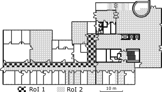
Figure 3: Two RoIs within one floor of an office building.

We kinematically determined the RFM by recording data approximately every 1.5 seconds while a user walked through the RoI and a total station tracked a prism attached to the Nexus smart phone with an accuracy of about 5 mm. The recording rate is around 0.67 Hz. This is higher than typically reported update rates for WLAN RSS and was achievable on this device by changing the hardware settings of the scanning interval. At the online stage, the RSS collection can be further accelerated by incremental scanning as discussed in (Brouwers et al. 2014). This approach is a compromise between the high accuracy attainable by stop & go measurements at carefully selected reference positions and the low extra effort of crowd-sourced RFM data collection as outlined e.g., in (Radu and Marina 2013). For simplicity we do not apply further pre-processing, such as filtering out the APs yielding low RSS values, discarding rarely measured APs, or merging signals transmitted from the same signal source on multi-frequencies although such steps could further reduce the computational complexity and improve the results in a real application.

In order to evaluate the performance of the proposed approach independently an additional test dataset was collected. The coordinates of the test positions (TPs) as measured by the total station were later used as ground truth for calculating the positioning error in terms of the Euclidean distances between estimated and true coordinates. The use of the tracking total station for both RFM data collection and test point data collection meant that RSS data did not have to be collected at any specific points (e.g. marked ones) within the RoI or subregions, and it was not necessary to occupy the same points again. We report the $\mathrm{50^{th}}$, $\mathrm{75^{th}}$ and $\mathrm{90^{th}}$ percentile of the horizontal positioning error (i.e. circular error (CE)50, CE75, CE90) defined as the minimum radius for including 50%, 75%, and 90% of the positioning errors (Potort et al. 2018). Furthermore, as an indicator for outlying position estimates (in particular due to wrong subregion selection) we also report the percentage of positioning errors exceeding 10 m, and as an indicator of computational complexity the average time to calculate the position of the test point. Data processing according to the proposed algorithms was implemented in Python using the scikit-learn package (Pedregosa et al. 2011) as outlined in Figure 1.

The details for two RoIs are summarized in Table 6 and the numbers of available features (i.e. visible WLAN APs or BLE beacons) are illustrated in Figure 5. The number of available features changes throughout the RoI and is thus also different in the different subregions. . Abrupt changes of feature observability occur in some locations close to walls and close to support pillars or cable/pipe ducts (not contained in the available floorplan). This is caused by the uneven number of raw measurements assigned to each subregion. In RoI 1, we carried out 5-rounds of one-day data collections about one month apart. This allowed us to take both the spatial and temporal variations into account when building the RFM. For RoI 2, the collected RFM is used as an example for validating the performance the proposed approach in case of a more extended RoI. Though the area of RoI 1 is a subset of RoI 2, the two RFMs are collected at different time and with different WLAN configurations . Both RoIs are divided into subregions of size $2\times 2m^{2}$ aligned with the floor plan of the RoI. While such an alignment may not be necessary, it is useful as it assures that individual subregions are not split by walls or other obstacles possibly causing discontinuities in the feature space. In many applications of an FIPS a floor plan exists, and can thus be used for subregion definition, because it is required for the FIPS and the associated location-based services anyway. In addition, some subregions contain no measurements (see Table 6). We have no need to treat the empty subregions specifically because they will be filtered out by subregion selection anyway without increasing the computational burden much.

The originally observed RFM of each subregion is further densified to a regular grid of about 25 reference points per $m^{2}$ (i.e. spacing about $0.2\times 0.2m^{2}$) by kernel smoothing interpolation (Figure 4) to mitigate the non-uniform point density of the original RFM (Figure 1). This process also ensures that data are available at the same location within one subregion. In this paper, we use a Matérn kernel (the length scale is 1) for smoothing the spatial distribution of the RSS and assume that the propagation channel introduces the additive Gaussian white noise to the RSS. The smoothly interpolated raw measurements are rounded to integers for reducing the storage requirements and for mitigating the impact of the quantization of RSS values on the positioning performance (Torres-Sospedra and Moreira 2017) and the APs are treated as non-measurable if their RSS values are lower than -100 dBm. The resulting gridded RFM is used for all further processing steps.

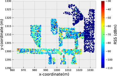
(a) Raw RSS

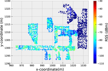
(b) Kernel smoothed RSS

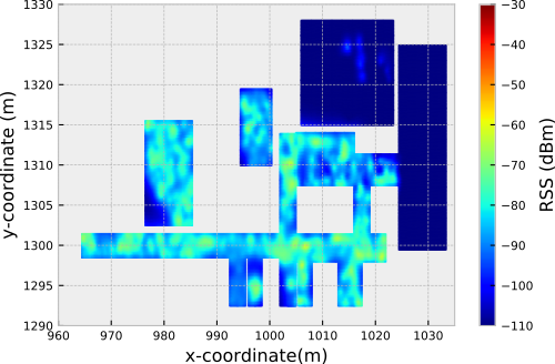
(c) Interpolated RSS ( $0.2\times 0.2m^{2}$ grid)

Figure 4: An example of the spatial distribution of RSS values as used for RFM generation

Table 6: Summary of RFM characteristics

RoI	Area ($m^{2}$)	Number of subregions	Number of features		Training data	Test data
			WLAN	BLE
1	120	35 (34)	399	–	1525	509
2	1100	326 (285)	490	278	2855	476

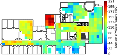
(a) Using RSS from WLAN APs as the features

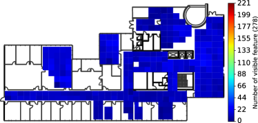
(b) Using RSS from BLE beacons as the features

Figure 5: The number of the available features of each subregion

4.2 Analysis using WLAN signals in RoI 1

4.2.1 Validation MJI-based subregion selection

The RoI 1 consists of 34 subregions. Figure 6a shows the MJI for all pairs of subregions indicating that the index is related to the Euclidean distance of the training data. This corresponds to the expectation that the same APs are available in nearby subregions while different APs are observed in subregions far from each other.

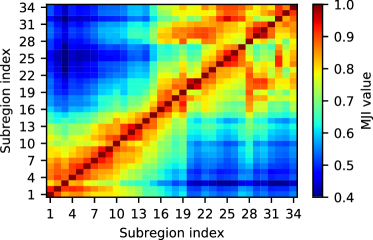
(a)

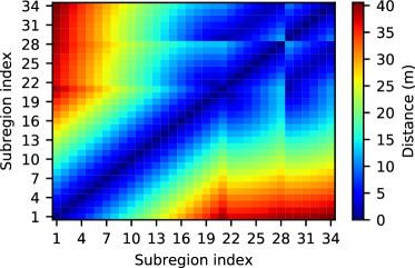
(b)

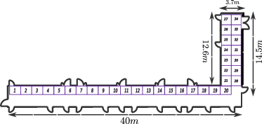
(c)

Figure 6: Analysis of MJI between the subregions of RoI 1 (training data). (a): Spatial distribution of the MJI. Apparent abrupt changes of MJI values appear in the up-right part. This is related to the spatial distribution of the subregions. (b) Spatial distribution of the distance. (c) Schematic of subregion division. Each subregion is indexed by an integer for this analysis. The concrete number associated with a specific subregion is irrelevant.

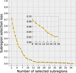
(a) RoI 1 (WLAN)

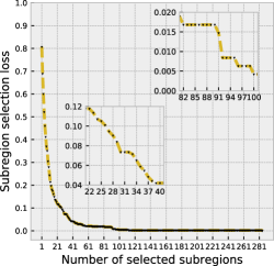
(b) RoI 2 (WLAN)

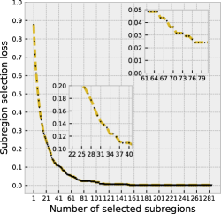
(c) RoI 2 (BLE)

Figure 7: The subregion selection loss with respect to the number of selected subregions

The MJI value is used here as an indicator of the similarity between the features measured by the user and the ones available in the individual subregions according to the RFM. We now use the loss function (2) to determine a suitable number $m$ of subregions for the MJI-based subregion selection. Figure 7a shows the loss as a function of $m$ for RoI 1. The figure indicates that the loss is almost constant if $m$ exceeds 16. In consecutive parts of this subsection, we analyze the performance of feature selection and positioning accuracy w.r.t. a given value of $m\in\{11,16,21,34\}$. In this range of $m$, we show that a small compromise of subregion selection accuracy does not harm the positioning accuracy too much, which is comparable to that obtained without subregion selection, i.e. for $m=34$ in RoI 1.

Table 7: The selected features of subregion 17. (The unique identification of AP is indexed from 0 to 398.)

Feature selection method	Positioning method	Selected features (top 5)
Randomized LASSO	–	13, 107, 9, 80, 11
Forward greedy search	$k$NN	11, 270, 272, 144, 19
	MAP	10, 398, 19, 20, 25
AFBGS	$k$NN	71, 11, 270, 272, 99
	MAP	66, 71, 12, 140, 272

4.2.2 Validation of AFBGS-based feature selection

In this part, we compare the feature selection performance using randomized LASSO as proposed in (Zhou and Wieser 2018b) to feature selection using the forward greedy algorithm and the AFBGS proposed herein. Since the latter two are directly related to fingerprinting-based positioning we evaluate the feature selection performance through the MSE of the position estimates calculated using the selected features. In Figure 8, we illustrate the MSE for two arbitrarily selected subregions using $k$NN and MAP. Regardless of the fingerprinting-based positioning method and subregion, all the curves in this figure have a similar pattern. We see that i) the MSE values achieved after applying forward search and AFBGS-based feature selection converge faster and more consistently than after applying randomized LASSO-based feature selection, and ii) randomized LASSO-based selection performance stabilizes with only a large number of selected features (e.g., $>20$). One explanation of this pattern is that randomized LASSO selects the features based on a regularized linear regression model instead of taking the fingerprinting-based positioning methods into account. However, if a higher number of features is used for positioning, the contribution of feature selection becomes less critical.

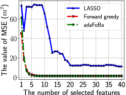
(a) $k$NN, subregion 11

(b) MAP, subregion 11

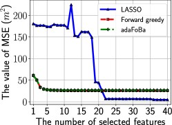
(c) $k$NN, subregion 21

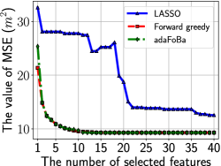
(d) MAP, subregion 21

Figure 8: The MSE paths of two subregions. In above test, the number of the selected subregion is fixed, i.e. $m=21$.

The difference of MSE between forward greedy search and AFBGS-based feature selection is very small (Figure 8), because the selected features are very similar in both cases, see Table 7. However, the AFBGS-based results are slightly better and we thus recommend it because of the increased flexibility.

4.2.3 The processing time and positioning accuracy

Table 8 presents the processing time for positioning one TP of RoIs 1 using WLAN signals as the features. The positioning time of MAP based on the AFBGS selected features within 21 selected subregions is about 2.9 seconds, which is almost 10 times faster than that of using all features for positioning by searching over all the subregions. The positioning time is also lower than when using LASSO for feature selection. One explanation is that a lower number of features is selected as relevant by the proposed algorithms than by LASSO, as shown in Figure 8. As for the positioning performance, the $\mathrm{90^{th}}$ percentile of the circular error (CE90) increases by less than 0.7 m for both MAP and MAP based on the AFBGS selected features within 9 selected subregions as compared to that of using all features for positioning and searching over the whole RoI. In addition, the resampling and the subregion selection reduce the percentage of large errors. So the reduced processing effort comes at the price of a small loss in accuracy. If need be, the percentage of outlying position estimates could be further reduced by position filtering taking the user’s motion or prior knowledge like floor plans into account during subregion selection and position estimation. This is beyond the scope of this paper and thus not further investigated here.

Table 8: Comparison of positioning times and accuracies of RoI 1 ($h=-1$ denotes that the all the relevant features within the selected subregions are used for positioning. These features are selected adaptively by AFBGS (see Section 3.3) ; their number is thus different for different subregions.)

Methods	Values of $(m,h)$	Mean positioning time (s)	CE50 (m)	CE75 (m)	CE90 (m)	Ratio of large errors (%)
MAP (without interpolation)	all	1.6	2.4	5.1	8.0	6.9
$k$NN (without interpolation)	all	$2.1\times 10^{-2}$	1.8	3.8	7.0	4.5
MAP (with interpolation)	all	34.7	2.2	4.9	8.0	5.5
$k$NN (with interpolation)	all	0.1	1.8	4.0	6.8	3.7
MAP (LASSO)	(11, -1)	2.4	2.9	5.4	9.0	8.6
	(16, -1)	4.3	2.6	5.3	9.2	8.6
	(21, -1)	6.5	2.7	5.3	9.2	8.6
	(34, -1)	11.6	2.5	5.0	8.8	8.6
	(34, 399)	34.7	2.2	4.9	8.0	5.5
$k$NN (LASSO)	(11, -1)	0.3$\times 10^{-2}$	2.2	4.5	7.5	4.1
	(16, -1)	0.5$\times 10^{-2}$	2.3	4.3	7.4	4.7
	(21, -1)	0.6$\times 10^{-2}$	2.0	4.2	7.3	4.9
	(34, -1)	1.0$\times 10^{-2}$	2.2	4.0	7.1	4.7
	(34, 399)	1.0$\times 10^{-2}$	1.8	3.9	6.9	4.5
MAP (Forward greedy search)	(11, -1)	1.4	2.7	5.3	8.6	7.1
	(16, -1)	2.5	2.7	5.6	9.2	8.4
	(21, -1)	3.9	2.7	5.6	9.4	8.8
	(34, -1)	6.9	2.7	5.5	9.3	8.3
	(34, 399)	34.9	2.4	5.2	8.2	6.3
$k$NN (Forward greedy search)	(11, -1)	0.2$\times 10^{-2}$	2.5	4.8	7.5	4.7
	(16, -1)	0.3$\times 10^{-2}$	2.8	5.1	8.2	5.5
	(21, -1)	0.3$\times 10^{-2}$	2.5	4.7	7.7	5.7
	(34, -1)	0.5$\times 10^{-2}$	2.3	4.7	8.4	5.3
	(34, 399)	1.0$\times 10^{-2}$	1.9	4.0	7.1	4.1
MAP (AFBGS)	(11, -1)	1.3	2.6	5.0	8.6	6.9
	(16, -1)	2.4	2.7	5.5	9.2	8.1
	(21, -1)	3.7	2.8	5.5	9.1	8.4
	(34, -1)	6.6	2.7	5.7	9.2	8.3
	(34, 399)	35.0	2.3	5.2	8.0	5.9
$k$NN (AFBGS)	(11, -1)	0.2$\times 10^{-2}$	2.9	5.0	7.4	4.5
	(16, -1)	0.3$\times 10^{-2}$	3.2	5.5	8.2	4.5
	(21, -1)	0.3$\times 10^{-2}$	2.7	5.3	8.1	5.1
	(34, -1)	0.4$\times 10^{-2}$	2.8	5.0	8.7	7.1
	(34, 399)	1.0$\times 10^{-2}$	1.8	4.0	6.8	3.7

4.3 Analysis using WLAN and BLE signals in RoI 2

In the larger RoI 2 both WLAN and BLE signals are extracted as fingerprints. In this subsection, we present the results of applying the proposed algorithm to that RoI and both signal types. As shown in Figure 7b and Figure 7c, MJI-based subregion selection is applicable also in this case. The figure indicates that there is no need to search within all subregions, but actually a subset is sufficient. Appropriate numbers of the selected subregions are 32 and 38 for using WLAN and BLE signals, respectively. These search spaces are less than 12% of the area of the RoI.

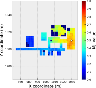
(a) WLAN

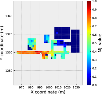
(b) BLE

Figure 9: Examples resulting in large subregion selection error. In the figure, the white color filled pentagon indicates the ground truth of the TPs.

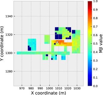
(a) WLAN

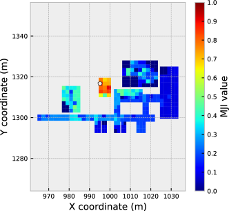
(b) BLE

Figure 10: Examples resulting in small subregion selection error. In the figure, the white color filled pentagon indicates the ground truth of the TPs.

Figure 7 also shows that there is a small fraction of test points (e.g. about 7% for WLAN signals and RoI 2) for which the correct subregion is not among the selected ones even when choosing 30 subregions. This may seem astonishing, but an investigation of the related test cases (see e.g., Figure 10) shows that this occurs mostly in cases where the gradient of the MJI within an extended neighborhood of the test point is small. In that case a few or individual additional or missing features can significantly influence the ranking of the subregions in terms of MJI. We observe and need to expect this case in larger, unobstructed areas like a hall without large furniture where there is little variability in the IDs of the features observed (e.g., the visible APs in case of WLAN RSS). This characteristic suggests that an augmented scheme of selecting the subregions is required for future work, e.g. selecting an adaptive number of subregions according to the spatial gradient of the MJI, dividing the subregions of varying size, or including the feature values for subregion selection in areas with little variability.

We present the positioning results of MAP and $k$NN using WLAN and BLE signals as the features in Table 9 and Table 10, respectively . We conclude from the results that the proposed subregion and feature selections are beneficial for the positioning with respect to constraining the online positioning by reducing the processing time and increasing the positioning accuracy. In fact, the circular errors CE50, CE75, and CE90 as defined above get smaller and the percentage of errors larger than 10 m reduces.

Table 9: Comparison of positioning times and accuracies of RoI 2 using WLAN signal as the features ($h=-1$ has the same meaning as in Table 8.)

Methods	Values of $(m,h)$	Mean positioning time (s)	CE50 (m)	CE75 (m)	CE90 (m)	Ratio of large errors (%)
MAP (without interpolation)	all	17.9	3.3	6.5	9.7	9.3
$k$NN (without interpolation)	all	0.1	1.6	3.1	4.8	1.7
MAP (with interpolation)	all	337.5	2.6	5.6	8.6	7.4
$k$NN (with interpolation)	all	0.30	1.4	2.6	4.6	1.9
MAP (LASSO)	(11, -1)	3.8	3.1	5.6	8.7	7.4
	(16, -1)	7.0	3.3	5.9	8.7	6.5
	(21, -1)	10.0	3.4	6.4	9.2	8.0
	(34, -1)	20.3	3.2	6.4	9.4	8.6
	(34, 490)	43.7	2.6	5.1	8.1	6.1
$k$NN (LASSO)	(11, -1)	0.6$\times 10^{-2}$	2.3	4.2	7.2	4.2
	(16, -1)	0.8$\times 10^{-2}$	2.3	4.3	6.8	4.0
	(21, -1)	1.0$\times 10^{-2}$	2.2	4.1	6.9	4.6
	(34, -1)	1.6$\times 10^{-2}$	2.3	4.2	6.6	4.4
	(34, 490)	1.3$\times 10^{-2}$	1.3	2.6	4.7	1.9
MAP (Forward greedy search)	(11, -1)	3.5	2.4	4.4	7.5	4.6
	(16, -1)	6.2	2.4	4.7	7.7	5.0
	(21, -1)	9.2	2.5	4.7	7.6	4.4
	(34, -1)	17.7	2.7	5.4	8.6	6.5
	(34, 490)	43.0	2.7	5.1	8.1	6.1
$k$NN (Forward greedy search)	(11, -1)	0.4$\times 10^{-2}$	2.5	4.3	7.0	3.4
	(16, -1)	0.5$\times 10^{-2}$	2.3	4.5	6.9	5.5
	(21, -1)	0.6$\times 10^{-2}$	2.2	4.3	7.4	5.7
	(34, -1)	0.8$\times 10^{-2}$	2.0	3.9	6.3	3.8
	(34, 490)	1.3$\times 10^{-2}$	1.3	2.6	4.3	2.1
MAP (AFBGS)	(11, -1)	3.4	2.6	4.6	7.4	5.0
	(16, -1)	6.4	2.6	5.2	7.9	5.9
	(21, -1)	10.3	2.7	5.1	7.9	5.7
	(34, -1)	22.5	2.8	5.2	8.4	5.5
	(34, 490)	46.2	2.7	5.0	8.0	5.9
$k$NN (AFBGS)	(11, -1)	0.6$\times 10^{-2}$	2.5	4.1	6.8	3.6
	(16, -1)	0.7$\times 10^{-2}$	2.5	4.5	7.2	4.2
	(21, -1)	0.8$\times 10^{-2}$	2.4	4.3	6.8	3.6
	(34, -1)	1.2$\times 10^{-2}$	2.0	4.0	6.4	2.5
	(34, 490)	2.3$\times 10^{-2}$	1.3	2.6	4.5	2.1

Table 10: Comparison of positioning times and accuracies of RoI 2 using BLE signal as the features ($h=-1$ has the same meaning as in Table 8.)

Methods	Values of $(m,h)$	Mean positioning time (s)	CE50 (m)	CE75 (m)	CE90 (m)	Ratio of large errors (%)
MAP (without interpolation)	all	5.9	5.2	9.7	17.1	23.6
$k$NN (without interpolation)	all	$2.6\times 10^{-2}$	3.4	6.5	9.8	9.5
MAP (with interpolation)	all	197.0	4.7	8.6	12.3	13.7
$k$NN (with interpolation)	all	0.1	3.4	6.9	11.3	12.2
MAP (LASSO)	(11, -1)	2.0	3.8	7.8	11.0	13.1
	(16, -1)	3.1	4.0	8.0	11.3	12.9
	(21, -1)	4.4	4.2	8.0	11.7	14.4
	(34, -1)	8.0	4.2	8.1	12.5	15.3
	(34, 278)	23.5	4.3	8.4	13.4	15.8
$k$NN (LASSO)	(11, -1)	0.4$\times 10^{-2}$	3.3	6.0	10.2	10.9
	(16, -1)	0.5$\times 10^{-2}$	3.2	6.6	10.3	11.2
	(21, -1)	0.6$\times 10^{-2}$	3.3	6.3	10.4	11.2
	(34, -1)	0.9$\times 10^{-2}$	3.3	6.5	10.5	11.4
	(34, 278)	0.9$\times 10^{-2}$	3.4	6.6	10.4	11.7
MAP (Forward greedy search)	(11, -1)	0.9	3.6	7.5	10.5	12.2
	(16, -1)	1.4	3.9	7.8	11.2	12.7
	(21, -1)	2.1	4.1	8.1	11.5	12.9
	(34, -1)	3.9	4.0	8.2	12.6	15.1
	(34, 278)	23.5	3.9	8.3	12.6	15.1
$k$NN (Forward greedy search)	(11, -1)	0.2$\times 10^{-2}$	4.1	7.4	11.3	12.9
	(16, -1)	0.3$\times 10^{-2}$	4.4	7.6	12.4	15.6
	(21, -1)	0.3$\times 10^{-2}$	4.4	8.1	12.6	18.0
	(34, -1)	0.4$\times 10^{-2}$	4.7	8.8	13.5	20.9
	(34, 278)	0.9$\times 10^{-2}$	3.3	6.4	10.7	11.2
MAP (AFBGS)	(11, -1)	1.0	3.6	7.4	10.9	13.1
	(16, -1)	1.7	3.8	7.8	11.7	13.6
	(21, -1)	2.5	3.9	8.0	11.9	14.1
	(34, -1)	5.1	4.0	8.3	12.8	15.6
	(34, 278)	23.5	4.3	8.3	12.9	15.1
$k$NN (AFBGS)	(11, -1)	0.2$\times 10^{-2}$	4.1	7.3	11.6	14.4
	(16, -1)	0.3$\times 10^{-2}$	4.3	7.9	12.2	17.0
	(21, -1)	0.3$\times 10^{-2}$	4.7	8.7	12.5	19.2
	(34, -1)	0.4$\times 10^{-2}$	4.8	8.6	12.6	18.5
	(34, 278)	0.9$\times 10^{-2}$	3.3	6.6	10.2	10.9

5 Conclusion

We proposed herein an approach to fingerprinting-based indoor positioning using opportunistically measured WLAN and BLE signals as the features for coordinate estimation. The main contributions are proposals to reduce data storage requirements and computational complexity in terms of processing time by segmentation of the entire region of interest (RoI) into subregions, identification of a few candidate subregions during the online positioning stage, and use of a selected subset of relevant features instead of all available features for position estimation. Subregion selection is based on a modified Jaccard index quantifying the similarity between the features obtained by the user and those available within the RFM. Feature selection is based on an adaptive forward-backward greedy search yielding a pre-computed set of relevant features for each subregion. The reduction of computational complexity is obtained both from the reduction of the number of candidate locations needed to analyze during online positioning and from the reduction of the number of features to be compared.

The experimental results corroborated the claim of reduced complexity while indicating that the positioning accuracy is hardly reduced by subregion and feature selection for the small RoI and even improves for the large RoI. For both investigated RoIs, the time required for the position estimation in the online stage was reduced by a factor of about 10 when using the selected relevant features within 11 selected subregions instead of using all features and searching over the entire RoI. For the small RoI (i.e. RoI 1), the increment of the $\mathrm{90^{th}}$ percentile errors (CE90) is 7.5% (i.e. 8.6 m instead of 8.0 m). In the large RoI (i.e. RoI 2), the positioning accuracy using MAP reduces from 9.8 m to 7.4 m for WLAN signals and from 12.3 m to 10.9 m for BLE. For $k$NN, the positioning accuracy does not change with subregion and feature selection. Given a fixed number of candidate subregions and a fixed, low number of features the computational burden of the entire algorithm is almost independent of the size of the entire RoI and of the number of available features across the RoI.

Future research will concentrate on investigating the role of subregion definition (shape, orientation, homogeneity) and possible benefit of optimization, on taking into account a user motion model during subregion selection, on handling temporal changes of the reference fingerprinting map, and on fully integrating different types of features for improving the positioning accuracy.

References

- Barron et al. (2008) Barron, A. R., A. Cohen, W. Dahmen, and R. A. DeVore (2008). Approximation and learning by greedy algorithms. The Annals of Statistics 36(1), 64–94.
- Bekkali et al. (2007) Bekkali, A., H. Sanson, and M. Matsumoto (2007). Rfid indoor positioning based on probabilistic rfid map and kalman filtering. In Wireless and Mobile Computing, Networking and Communications, 2007. WiMOB 2007. Third IEEE International Conference on, pp. 21–21. IEEE.
- Berlinet and Thomas-Agnan (2011) Berlinet, A. and C. Thomas-Agnan (2011). Reproducing Kernel Hilbert Spaces in Probability and Statistics. Berlin Heidelberg: Springer Science & Business Media.
- Bishop (2006) Bishop, C. M. (2006). Pattern Recognition and Machine Learning (Information Science and Statistics). Berlin, Heidelberg: Springer-Verlag.
- Bisio et al. (2014) Bisio, I., M. Cerruti, F. Lavagetto, M. Marchese, M. Pastorino, A. Randazzo, and A. Sciarrone (2014). A Trainingless WiFi Fingerprint Positioning Approach Over Mobile Devices. IEEE Antennas and Wireless Propagation Letters 13, 832–835.
- Bisio et al. (2013) Bisio, I., F. Lavagetto, M. Marchese, and A. Sciarrone (2013, July). Performance comparison of a probabilistic fingerprint-based indoor positioning system over different smartphones. In 2013 International Symposium on Performance Evaluation of Computer and Telecommunication Systems (SPECTS), pp. 161–166.
- Bisio et al. (2016) Bisio, I., F. Lavagetto, M. Marchese, and A. Sciarrone (2016, September). Smart probabilistic fingerprinting for WiFi-based indoor positioning with mobile devices. Pervasive and Mobile Computing 31, 107–123.
- Brouwers et al. (2014) Brouwers, N., M. Zuniga, and K. Langendoen (2014, March). Incremental Wi-Fi scanning for energy-efficient localization. In 2014 IEEE International Conference on Pervasive Computing and Communications (PerCom), pp. 156–162.
- Bühlmann (2006) Bühlmann, P. (2006, 04). Boosting for high-dimensional linear models. Ann. Statist. 34(2), 559–583.
- Chen et al. (2006) Chen, Y., Q. Yang, J. Yin, and X. Chai (2006). Power-efficient access-point selection for indoor location estimation. IEEE Transactions on Knowledge and Data Engineering 18(7), 877–888.
- Driusso et al. (2016) Driusso, M., C. Marshall, M. Sabathy, F. Knutti, H. Mathis, and F. Babich (2016, Oct). Indoor positioning using lte signals. In 2016 International Conference on Indoor Positioning and Indoor Navigation (IPIN), pp. 1–8.
- El-Kafrawy et al. (2010) El-Kafrawy, K., M. Youssef, A. El-Keyi, and A. Naguib (2010). Propagation modeling for accurate indoor WLAN RSS-based localization. IEEE Vehicular Technology Conference, 1–5.
- Fastrich et al. (2015) Fastrich, B., S. Paterlini, and P. Winker (2015). Constructing optimal sparse portfolios using regularization methods. Computational Management Science 12(3), 417–434.
- Feng et al. (2012) Feng, C., W. S. A. Au, S. Valaee, and Z. Tan (2012). Received-signal-strength-based indoor positioning using compressive sensing. IEEE Transactions on Mobile Computing 11(12), 1983–1993.
- Gu et al. (2017) Gu, Y., C. Zhou, A. Wieser, and Z. Zhou (2017, Sept). Wifi based trajectory alignment, calibration and crowdsourced site survey using smart phones and foot-mounted imus. In 2017 International Conference on Indoor Positioning and Indoor Navigation (IPIN), pp. 1–6.
- Hazas and Hopper (2006) Hazas, M. and A. Hopper (2006). Broadband ultrasonic location systems for improved indoor positioning. IEEE Transactions on mobile Computing 5(5), 536–547.
- He and Chan (2016) He, S. and S.-H. G. Chan (2016). Wi-fi fingerprint-based indoor positioning: Recent advances and comparisons. IEEE Communications Surveys & Tutorials 18(1), 466–490.
- Huang and Manh (2016) Huang, C. C. and H. N. Manh (2016). RSS-Based Indoor Positioning Based on Multi-Dimensional Kernel Modeling and Weighted Average Tracking. IEEE Sensors Journal 16(9), 3231–3245.
- Ingram et al. (2004) Ingram, S., D. Harmer, and M. Quinlan (2004). Ultrawideband indoor positioning systems and their use in emergencies. In Position Location and Navigation Symposium (PLANS), pp. 706–715. IEEE.
- Jani et al. (2015) Jani, S. S., J. M. Lamb, B. M. White, M. Dahlbom, C. G. Robinson, and D. A. Low (2015, Jan). Assessing margin expansions of internal target volumes in 3d and 4d pet: a phantom study. Annals of Nuclear Medicine 29(1), 100–109.
- Jun et al. (2017) Jun, J., L. He, Y. Gu, W. Jiang, G. Kushwaha, V. A, L. Cheng, C. Liu, and T. Zhu (2017). Low-Overhead WiFi Fingerprinting. IEEE Transactions on Mobile Computing 1233(c), 1–14.
- Jung et al. (2011) Jung, S., C. oh Lee, and D. Han (2011, Aug). Wi-fi fingerprint-based approaches following log-distance path loss model for indoor positioning. In 2011 IEEE MTT-S International Microwave Workshop Series on Intelligent Radio for Future Personal Terminals, pp. 1–2.
- Kalbandhe and Patil (2016) Kalbandhe, A. A. and S. C. Patil (2016, Dec). Indoor positioning system using bluetooth low energy. In 2016 International Conference on Computing, Analytics and Security Trends (CAST), pp. 451–455.
- Karegar (2017) Karegar, P. A. (2017, Apr). Wireless fingerprinting indoor positioning using affinity propagation clustering methods. Wireless Networks.
- Kasprzak et al. (2013) Kasprzak, S., A. Komninos, and P. Barrie (2013, July). Feature-based indoor navigation using augmented reality. In 2013 9th International Conference on Intelligent Environments, pp. 100–107.
- Khalajmehrabadi et al. (2017) Khalajmehrabadi, A., N. Gatsis, and D. Akopian (2017, July). Structured group sparsity: A novel indoor wlan localization, outlier detection, and radio map interpolation scheme. IEEE Transactions on Vehicular Technology 66(7), 6498–6510.
- Kushki et al. (2007) Kushki, A., K. N. Plataniotis, and A. N. Venetsanopoulos (2007, June). Kernel-based positioning in wireless local area networks. IEEE Transactions on Mobile Computing 6(6), 689–705.
- Kushki et al. (2010) Kushki, A., K. N. Plataniotis, and A. N. Venetsanopoulos (2010, March). Intelligent dynamic radio tracking in indoor wireless local area networks. IEEE Transactions on Mobile Computing 9(3), 405–419.
- Ledlie et al. (2011) Ledlie, J., J. g. Park, D. Curtis, A. Cavalcante, L. Camara, A. Costa, and R. Vieira (2011, Sept). Mole: A scalable, user-generated wifi positioning engine. In 2011 International Conference on Indoor Positioning and Indoor Navigation, pp. 1–10.
- Lee et al. (2004) Lee, C., Y. Chang, G. Park, J. Ryu, S.-G. Jeong, S. Park, J. W. Park, H. C. Lee, K. shik Hong, and M. H. Lee (2004, Nov). Indoor positioning system based on incident angles of infrared emitters. In 30th Annual Conference of IEEE Industrial Electronics Society (IECON), Volume 3, pp. 2218–2222.
- Li et al. (2013) Li, L., W. Yang, and G. Wang (2013, July). Hiwl: An unsupervised learning algorithm for indoor wireless localization. In 2013 12th IEEE International Conference on Trust, Security and Privacy in Computing and Communications, pp. 1747–1753.
- Madigan et al. (2005) Madigan, D., E. Einahrawy, R. P. Martin, W. H. Ju, P. Krishnan, and A. S. Krishnakumar (2005, March). Bayesian indoor positioning systems. In Proceedings IEEE 24th Annual Joint Conference of the IEEE Computer and Communications Societies., Volume 2, pp. 1217–1227.
- Mallat and Zhang (1993) Mallat, S. G. and Z. Zhang (1993, Dec). Matching pursuits with time-frequency dictionaries. IEEE Transactions on Signal Processing 41(12), 3397–3415.
- Mendoza-Silva et al. (2018) Mendoza-Silva, G., P. Richter, J. Torres-Sospedra, E. Lohan, and J. Huerta (2018). Long-Term WiFi Fingerprinting Dataset for Research on Robust Indoor Positioning. Data 3(1), 3.
- Mitchell (1997) Mitchell, T. M. (1997). Machine Learning (1 ed.). New York, NY, USA: McGraw-Hill, Inc.
- Nandakumar et al. (2012) Nandakumar, R., K. K. Chintalapudi, and V. N. Padmanabhan (2012). Centaur: Locating devices in an office environment. In Proceedings of the 18th Annual International Conference on Mobile Computing and Networking, Mobicom ’12, New York, NY, USA, pp. 281–292. ACM.
- Niedermayr et al. (2014) Niedermayr, S., A. Wieser, and H. Neuner (2014). Expressing location uncertainty in combined feature-based and geometric positioning. In Proceedings European Navigation Conference 2014, pp. 154–166. EUGIN.
- Nuño-Barrau and Páez-Borrallo (2006) Nuño-Barrau, G. and J. M. Páez-Borrallo (2006). A new location estimation system for wireless networks based on linear discriminant functions and hidden markov models. Eurasip Journal on Applied Signal Processing 2006, 1–17.
- Ouyang et al. (2012) Ouyang, R. W., A. K. S. Wong, C. T. Lea, and M. Chiang (2012, Nov). Indoor location estimation with reduced calibration exploiting unlabeled data via hybrid generative/discriminative learning. IEEE Transactions on Mobile Computing 11(11), 1613–1626.
- Padmanabhan et al. (2000) Padmanabhan, P. B., V. N., and V. N. (2000). RADAR: An in-building RF based user location and tracking system. Proceedings IEEE INFOCOM 2000. Conference on Computer Communications. Nineteenth Annual Joint Conference of the IEEE Computer and Communications Societies (Cat. No.00CH37064) 2(c), 775–784.
- Park et al. (2010) Park, J.-g., B. Charrow, D. Curtis, J. Battat, E. Minkov, J. Hicks, S. Teller, and J. Ledlie (2010). Growing an organic indoor location system. In Proceedings of the 8th international conference on Mobile systems, applications, and services, pp. 271–284. ACM.
- Park and Casella (2008) Park, T. and G. Casella (2008). The bayesian lasso. Journal of the American Statistical Association 103(482), 681–686.
- Pedregosa et al. (2011) Pedregosa, F., G. Varoquaux, A. Gramfort, V. Michel, B. Thirion, O. Grisel, M. Blondel, P. Prettenhofer, R. Weiss, V. Dubourg, J. Vanderplas, A. Passos, D. Cournapeau, M. Brucher, M. Perrot, and E. Duchesnay (2011). Scikit-learn: Machine learning in Python. Journal of Machine Learning Research 12, 2825–2830.
- Potort et al. (2018) Potort, F., A. Crivello, P. Barsocchi, and F. Palumbo (2018). Evaluation of indoor localisation systems : comments on the ISO / IEC 18305 standard. (September), 24–27.
- Radu and Marina (2013) Radu, V. and M. K. Marina (2013, Oct). Himloc: Indoor smartphone localization via activity aware pedestrian dead reckoning with selective crowdsourced wifi fingerprinting. In International Conference on Indoor Positioning and Indoor Navigation, pp. 1–10.
- Renaudin et al. (2018) Renaudin, O., T. Zemen, and T. Burgess (2018, jun). Ray-Tracing Based Fingerprinting for Indoor Localization. In 2018 IEEE 19th International Workshop on Signal Processing Advances in Wireless Communications (SPAWC), pp. 1–5.
- Saxena and Zawodniok (2014) Saxena, A. and M. Zawodniok (2014, May). Indoor positioning system using geo-magnetic field. In 2014 IEEE International Instrumentation and Measurement Technology Conference (I2MTC) Proceedings, pp. 572–577.
- Sorour et al. (2015) Sorour, S., Y. Lostanlen, S. Valaee, and K. Majeed (2015, May). Joint indoor localization and radio map construction with limited deployment load. IEEE Transactions on Mobile Computing 14(5), 1031–1043.
- Talvitie et al. (2015) Talvitie, J., M. Renfors, and E. S. Lohan (2015, April). Distance-based interpolation and extrapolation methods for rss-based localization with indoor wireless signals. IEEE Transactions on Vehicular Technology 64(4), 1340–1353.
- Tibshirani (1996) Tibshirani, R. (1996). Regression shrinkage and selection via the lasso. Journal of the Royal Statistical Society. Series B (Methodological), 267–288.
- Torres-Sospedra et al. (2014) Torres-Sospedra, J., R. Montoliu, A. Martínez-Usó, J. P. Avariento, T. J. Arnau, M. Benedito-Bordonau, and J. Huerta (2014, Oct). Ujiindoorloc: A new multi-building and multi-floor database for wlan fingerprint-based indoor localization problems. In 2014 International Conference on Indoor Positioning and Indoor Navigation (IPIN), pp. 261–270.
- Torres-Sospedra and Moreira (2017) Torres-Sospedra, J. and A. Moreira (2017). Analysis of Sources of Large Positioning Errors in Deterministic Fingerprinting. Sensors (Switzerland), 1–48.
- Torres-Sospedra et al. (2015) Torres-Sospedra, J., D. Rambla, R. Montoliu, O. Belmonte, and J. Huerta (2015, Oct). Ujiindoorloc-mag: A new database for magnetic field-based localization problems. In 2015 International Conference on Indoor Positioning and Indoor Navigation (IPIN), pp. 1–10.
- Wu et al. (2013) Wu, C., Z. Yang, Y. Liu, and W. Xi (2013, April). Will: Wireless indoor localization without site survey. IEEE Transactions on Parallel and Distributed Systems 24(4), 839–848.
- Wu et al. (2004) Wu, C.-L., L.-C. Fu, and F.-L. Lian (2004). Wlan location determination in e-home via support vector classification. In IEEE International Conference on Networking, Sensing and Control, 2004, Volume 2, pp. 1026–1031 Vol.2.
- Xie et al. (2016) Xie, H., T. Gu, X. Tao, H. Ye, and J. Lu (2016). A Reliability-Augmented Particle Filter for Magnetic Fingerprinting Based Indoor Localization on Smartphone. IEEE Transactions on Mobile Computing 15(8), 1877–1892.
- Yassin et al. (2017) Yassin, A., Y. Nasser, M. Awad, A. Al-Dubai, R. Liu, C. Yuen, R. Raulefs, and E. Aboutanios (2017). Recent Advances in Indoor Localization: A Survey on Theoretical Approaches and Applications. IEEE Communications Surveys Tutorials 19(2), 1327–1346.
- Youssef and Agrawala (2008) Youssef, M. and A. Agrawala (2008). The Horus location determination system. Wireless Networks 14(3), 357–374.
- Youssef et al. (2003) Youssef, M. A., A. Agrawala, and A. U. Shankar (2003). Wlan location determination via clustering and probability distributions. In Pervasive Computing and Communications, 2003.(PerCom 2003). Proceedings of the First IEEE International Conference on, pp. 143–150. IEEE.
- Zhang (2011) Zhang, T. (2011). Adaptive forward-backward greedy algorithm for learning sparse representations. IEEE transactions on information theory 57(7), 4689–4708.
- Zhou and Wieser (2018a) Zhou, C. and A. Wieser (2018a, Sept). CDM: Compound dissimilarity measure and an application to fingerprinting-based positioning. In 2018 International Conference on Indoor Positioning and Indoor Navigation (IPIN), pp. 1–7.
- Zhou and Wieser (2018b) Zhou, C. and A. Wieser (2018b). Jaccard Analysis and LASSO-Based Feature Selection for Location Fingerprinting with Limited Computational Complexity, pp. 71–87. Cham: Springer International Publishing.