Auxin transport model for leaf venation

Jan Haskovec  Henrik Jönsson  Lisa Maria Kreusser  Peter Markowich

Abstract. The plant hormone auxin controls many aspects of the development of plants. One striking dynamical feature is the self-organisation of leaf venation patterns which is driven by high levels of auxin within vein cells. The auxin transport is mediated by specialised membrane-localised proteins. Many venation models have been based on polarly localised efflux-mediator proteins of the PIN family. Here, we investigate a modeling framework for auxin transport with a positive feedback between auxin fluxes and transport capacities that are not necessarily polar, i.e. directional across a cell wall. Our approach is derived from a discrete graph-based model for biological transportation networks, where cells are represented by graph nodes and intercellular membranes by edges. The edges are not a-priori oriented and the direction of auxin flow is determined by its concentration gradient along the edge. We prove global existence of solutions to the model and the validity of Murray’s law for its steady states. Moreover, we demonstrate with numerical simulations that the model is able connect an auxin source-sink pair with a mid-vein and that it can also produce branching vein patterns. A significant innovative aspect of our approach is that it allows the passage to a formal macroscopic limit which can be extended to include network growth. We perform mathematical analysis of the macroscopic formulation, showing the global existence of weak solutions for an appropriate parameter range.

1. Introduction

The hormone auxin plays a central role in many developmental processes in plants [14, 33, 32, 31]. During the development of a leaf, a connected network of veins is formed in a highly predictable order, generating a well defined pattern in the final leaf [15]. High levels of auxin are present in the forming vein cells compared to the neighboring tissues. It has been shown that the membrane localized PIN-FORMED (PIN) family of auxin transport mediators is essential for the correct patterning of the vein network [29, 33]. The patterns could result from a canalisation mechanism where the auxin flux feeds back itself to a polarised transport connecting sources and sinks of auxin [30, 22, 23]. This idea has been revisited recently and has led to models with polarised PIN transporters [27, 11, 10]. No flux-sensing mechanism has been identified but models have been used to suggest alternatives [19, 5]. While newer models have solved the issue of unrealistically low levels of auxin within veins in flux-based models [11], it is still an open question how looped veins can form [27, 8] and if specified auxin production can provide an answer.

PIN proteins are involved in several patterning processes in plants. Alternative models, not based on auxin flux, have been proposed, for instance for producing Turing-like dynamics in the context of phyllotaxis [17, 36, 4], and for single cell polarity resulting in planar polarity [1].

Since the discovery of PINs, many venation models have been based on polarised transport via PINs, while recent data suggests that polar auxin transport mediated by PINs is not crucial for forming veins [32, 31]. Although characteristic vein patterns and leaf shapes can be obtained with these PIN-based models, veins can also form in chemical perturbations when PIN-mediated auxin transport is blocked, or when multiple membrane-localised PIN proteins are mutated. This raises the question if alternative mechanisms work in parallel or together with the PIN-based polar transporters during the initiation of veins. This motivates to consider a more general modelling approach where alternative feedbacks between auxin, auxin fluxes and auxin transport can be included.

The ultimate goal for modelling vein networks is to accurately predict vein network geometries seen in different plants. Our novel dynamical description could complement the PIN-based models which have focused on more basic dynamic patterns of veins, such as connecting sources and sinks, and breaking the symmetry of graded diffusion into veins. Examples of these PIN-based models include the traditional PIN-based flux models that have been studied since approximately 40 years, see [30, 22, 23]. The impact of auxin concentration on the pattern formation has been studied in [21]. It would be very interesting to investigate the emergence of patterns in the setting where PINs are removed. As noted above, the traditional PIN-based flux models are yet to provide a full description of the diverse patterns seen in plants.

Given the strong directional distribution of PINs and the ability of veins to form without PINs, it is important to introduce and analyse alternative mechanisms. Whether these mechanisms are identical/redundant to PIN mechanisms in terms of their dynamical behaviour or whether other mechanisms need to be considered is still unknown. Hence, it would be interesting to show that polar/directional transport activity and directional flux measurements are not required, and that vein-like patterns can also result from mere measurement of magnitudes. This may also inspire scientists to reconsider their current data or design new experiments.

In this paper we study a modeling framework for leaf venation which does not assume polarity of auxin transport mediators across cell walls. The model is introduced in Section 2, and is based on a positive feedback loop between auxin fluxes and transport capacities that are not necessarily polar. Our approach is derived from a recent discrete graph-based model for biological transportation networks introduced by Hu and Cai [16]. We represent cells by graph nodes and intercellular membranes (connections) by edges. The edges are not a-priori oriented and the direction of auxin flow is determined by its concentration gradient along the edge. The transport capacity of each edge is represented by the local concentration of the auxin mediator. Our approach can be understood as a modeling framework, which can be equipped or extended with various biologically relevant features that will produce experimentally testable hypotheses. We admit that in its present setting it does not capture all relevant biological features, however, its main advantage is a rather simple form that facilitates rigorous mathematical analysis. In particular, the first aim of this paper is the proof of global existence and nonnegativity of solutions of the discrete model (Section 3). Moreover, in Section 4 we show that the stationary solutions satisfy a generalized Murray’s law. The second aim of the paper is to gain a better understanding of the pattern formation capacity of the model by means of numerical simulations (Section 5). In particular, we show that it is capable of generating patterns connecting an auxin source-sink pair with a mid-vein and that it can produce branching vein patterns. The main novelty of our modelling approach is that it facilitates a (formal) passage to a continuum limit, which is the subject of Section 6. The resulting system of partial differential equations captures network growth and is expected to exhibit a rich patterning capacity (see [2] for results of numerical simulations of a related continuum model). Here we prove the existence of weak solutions of the transient problem and of its steady states.

2. Description of the model

Hu and Cai considered a discrete model describing the formation of generic biological transport networks in [16]. Existence of transient solutions, their qualitative properties and the formal continuum limit of the Hu and Cai model was studied in [13]. Here we adapt the model to the cellular context to describe auxin transport in plant leafs via transporter proteins, where the orientation of the flow is determined by auxin concentration gradient. Our approach shares many similarities with the one introduced by Mitchison in [22] where the transport capacity is updated as a function of the flux (gradient) between cells. However, while Mitchison suggested an asymmetric update of the transport capacities across a cell wall, our model assumes a symmetric transport capacity across a cell wall. In this section we shall first introduce the Hu and Cai model, then shortly discuss the Mitchison model, and finally describe the adaptation to the cellular context.

2.1. Model of Hu and Cai [16]

The discrete model introduced by Hu and Cai [16] and reformulated in [2] is posed on a given, fixed undirected connected graph $G=(V,E)$, consisting of a finite set of vertices $V$ of size $N=|V|$ and a finite set of edges $E$. Any pair of vertices is connected by at most one edge and no vertex is connected to itself. We denote the edge between vertices $i\in V$ and $j\in V$ by $(i,j)\in E$. Since the graph is undirected, $(i,j)$ and $(j,i)$ refer to the same edge. For each edge $(i,j)\in E$ of the graph $G$ we consider its length and its conductivity, denoted by $L_{ij}=L_{ji}>0$ and $C_{ij}=C_{ji}\geq 0$, respectively. The edge lengths $L_{ij}>0$ are given as a datum and fixed for all $(i,j)\in E$. With each vertex $i\in V$, the fluid pressure $P_{i}\in\mathbb{R}$ is associated. The pressure drop between vertices $i\in V$ and $j\in V$ connected by an edge $(i,j)\in E$ is given by

$$(\Delta P)_{ij}:=P_{j}-P_{i}.$$ (2.1)

Note that the pressure drop is antisymmetric, i.e., by definition, $(\Delta P)_{ij}=-(\Delta P)_{ji}$. The oriented flux (flow rate) from vertex $i\in V$ to $j\in V$ is denoted by $Q_{ij}$; again, we have $Q_{ij}=-Q_{ji}$. Since the Reynolds number of the flow is typically small for biological networks and the flow is predominantly laminar, the flow rate between vertices $i\in V$ and $j\in V$ along edge $(i,j)\in E$ is proportional to the conductance $C_{ij}$ and the pressure drop $(\Delta P)_{ij}=P_{j}-P_{i}$,

$$Q_{ij}:=C_{ij}\frac{P_{j}-P_{i}}{L_{ij}}\qquad\text{for all~{}}(i,j)\in E.$$ (2.2)

The local mass conservation in each vertex is expressed in terms of the Kirchhoff law

$$-\sum_{j\in\mathcal{N}(i)}C_{ij}\frac{P_{j}-P_{i}}{L_{ij}}=S_{i}\qquad\text{for all~{}}i\in V.$$ (2.3)

Here $\mathcal{N}(i)$ denotes the set of vertices connected to $i\in V$ through an edge, and $S=(S_{i})_{i\in V}$ is the prescribed strength of the flow source ($S_{i}>0$) or sink ($S_{i}<0$) at vertex $i$. Clearly, a necessary condition for the solvability of (2.3) is the global mass conservation

$$\sum_{i\in V}S_{i}=0,$$ (2.4)

which we assume in the following. Given the vector of conductivities $C=(C_{ij})_{(i,j)\in E}$, the Kirchhoff law (2.3) is a linear system of equations for the vector of pressures $P=(P_{i})_{i\in V}$. With the global mass conservation (2.4), the linear system (2.3) is solvable if and only if the graph with edge weights $C=(C_{ij})_{(i,j)\in E}$ is connected [2], where only edges with positive conductivities $C_{ij}>0$ are taken into account (i.e., edges with zero conductivities are discarded). Note that the solution is unique up to an additive constant.

The conductivities $C_{ij}$ are subject to an energy optimization and adaptation process. Hu and Cai [16] propose an energy cost functional consisting of a pumping power term and a metabolic cost term. According to Joule’s law, the power (kinetic energy) needed to pump material through an edge $(i,j)\in E$ is proportional to the pressure drop $(\Delta P)_{ij}=P_{j}-P_{i}$ and the flow rate $Q_{ij}$ along the edge, i.e., $(\Delta P)_{ij}Q_{ij}=\frac{Q_{ij}^{2}}{C_{ij}}L_{ij}$. The metabolic cost of maintaining the edge is assumed to be proportional to its length $L_{ij}$ and a power of its conductivity $C_{ij}^{\gamma}$, where the exponent $\gamma>0$ depends on the network. For models of leaf venation the material cost is proportional to the number of small tubes, which is proportional to $C_{ij}$, and the metabolic cost is due to the effective loss of the photosynthetic power at the area of the venation cells, which is proportional to $C_{ij}^{1/2}$. Consequently, the effective value of $\gamma$ typically used in models of leaf venation lies between $1/2$ and $1$; see [16]. The energy cost functional is thus given by

$${\mathcal{E}}[C]:=\sum_{(i,j)\in E}\left(\frac{Q_{ij}[C]^{2}}{C_{ij}}+\frac{\nu}{\gamma}C_{ij}^{\gamma}\right)L_{ij},$$ (2.5)

where $Q_{ij}[C]$ is given by (2.2) with pressures calculated from the Kirchhoff’s law (2.3), and $\nu>0$ is the so-called metabolic coefficient. Note that every edge of the graph $G$ is counted exactly once in the above sum. Hu and Cai [16] propose an energy optimization and adaptation process for the conductivities $C_{ij}$ based on the gradient flow of the energy (2.5),

$$\frac{\,\mathrm{d}C_{ij}}{\,\mathrm{d}t}=\sigma\left(\frac{Q_{ij}[C]^{2}}{C_{ij}^{\gamma+1}}-\tau^{2}\right)C_{ij}L_{ij}$$ (2.6)

with parameters $\sigma,\tau>0$, constrained by the Kirchhoff law (2.3), see [13] for details.

2.2. Mitchison model [23]

The model proposed by Mitchison [22] describes auxin dynamics within an array of cells with indices $i\in V$. For two cells $i,j\in V$ with signal concentrations $s_{i},s_{j}$, respectively, the diffusion constant at the interface between the cells is denoted by $D_{ij}=D_{ji}\geq 0$ and can be specified independently for each cell-cell interface. The oriented flux from vertex $i\in V$ to $j\in V$ is given by Fick’s law [6],

$$\phi_{ij}=D_{ij}\frac{s_{i}-s_{j}}{L_{ij}},$$ (2.7)

where $L_{ij}=L_{ji}>0$ denotes the (average) length of cells $i$ and $j$. In particular, we have $\phi_{ij}=-\phi_{ji}$. The dependence of the diffusion constant $D_{ij}$ on the flux $\phi_{ij}$ is of the form

$$\frac{\mathop{}\!\mathrm{d}D_{ij}}{\mathop{}\!\mathrm{d}t}=f(|\phi_{ij}|,D_{ij})$$

for a suitable function $f$ such that $|\phi_{ij}|/D_{ij}$ decreases as $|\phi_{ij}|$ increases. For instance, $f$ can be chosen such that $D_{ij}\approx\phi_{ij}^{2}$ for $\phi_{ij}>0$ and $D_{ij}=0$ for $\phi_{ij}\leq 0$, resulting in a strictly polar transport capacity across a cell wall. Assuming that cell $i\in V$ receives fluxes $\phi_{ji}$ for $j\in\mathcal{N}(i)$, the evolution of the signal $s_{i}$ is of the form

$$\frac{\mathop{}\!\mathrm{d}s_{i}}{\mathop{}\!\mathrm{d}t}=\sigma_{i}+\frac{1}{v}\sum_{j\in\mathcal{N}(i)}A_{ij}\phi_{ji}.$$ (2.8)

As before, $\mathcal{N}(i)$ denotes the index set of neighboring cells of cell $i\in V$. The parameter $\sigma_{i}$ is the source activity for signal production in cell $i\in V$. All cells have volume $v>0$ and $A_{ij}=A_{ji}>0$ is the area of the interface between cell $i$ and its neighbor $j\in\mathcal{N}(i)$. Note that the term $\sum_{j\in\mathcal{N}(i)}A_{ij}\phi_{ji}$ can be regarded as the difference between influx and outflux since $\phi_{ij}=-\phi_{ji}$ for $j\in\mathcal{N}(i)$. For the conservation of the signal we require that the source activity $\sigma_{i}$ for signal production and degradation is chosen such that $\frac{\mathop{}\!\mathrm{d}}{\mathop{}\!\mathrm{d}t}\sum_{i\in V}s_{i}=0.$

It is worth noting that while it was well established that auxin was important for generating the vascular or vein patterns (see, e.g., [30]), auxin ‘transporters’ were not identified at the time when the model was introduced. It received great attention only later, when auxin transport mediator proteins with similar polar localisation as predicted by the model were identified [33]. In particular, PIN proteins are integral membrane proteins that transport the anionic form of auxin across membranes. Most of the PIN proteins localize at the plasma membrane where they serve as secondary active transporters involved in the efflux of auxin. They show asymmetrical localizations on the membrane and are therefore responsible for polar auxin transport. Still, while PIN loss of function mutants generate phenotypes in venation patterns, they do not completely abolish the formation of veins [32], and as such alternative mechanisms can contribute to the dynamics of vein formation. While individual mutants do not show strong phenotypes, this is also implied by the existence of other auxin transport proteins, such as AUX1/LAX influx mediators [18, 26, 32], regulating intracellular and intercellular transport. In the following discussion we will often use PIN as a descriptor of the auxin transporter protein for simplicity, but it should be seen as a more general description of auxin transport mediated by polar and/or nonpolar membrane proteins, where polar relates to the difference of transport capacity (PIN localisation) on the two sides of a wall.

2.3. Adapted Hu-Cai model in cellular context

Given the known auxin flows generated from sources to sinks in a plant tissue, the sometimes clear expression but unclear polarisation of PIN auxin transporter proteins in these veins, and the ability to generate veins without any PIN transport, it is of interest to investigate alternative mechanisms for the vein dynamics in an auxin context. Such an alternative can be provided by a proper adaptation of the Hu and Cai model for transport networks [16]. The mechanism where pressure differences feed back on conductance between elements has similarity with the auxin transport case, as described in the flux-based models [22, 23]. Here auxin sources and concentration differences (pressure in the Hu-Cai model) generate diffusive fluxes between cells (spatial elements) that positively feed back on transport rates between the cells (conductance). To adapt the Hu-Cai model to a cellular context of plant venation dynamics we consider $n=|V|$ cells with indices $i\in V$ and replace the pressure $P_{i}$ at vertex $i\in V$ in the Hu-Cai model with the auxin concentration $a_{i}\geq 0$.

The conductance $C_{ij}$ of edge $(i,j)\in E$ in the Hu and Cai model is replaced by the transport activity $X_{ij}=X_{ji}\geq 0$ in the membrane connecting cells $i\in V$ and $j\in V$ which is the main difference from PIN-based flux models (and experiments) with PINs $\mathcal{P}_{ij}$ where $\mathcal{P}_{ij}\neq\mathcal{P}_{ji}$. Due to this modelling approach auxin transporters are not directional, i.e. polar, and as we shall see, measuring the magnitudes $X_{ij}$ is sufficient for producing vein-like dynamics. However, cells, in general, do not transport auxin equally well in all directions (i.e. $X_{ij}$ is typically not equal to $X_{ik}$ for two cell neighbours $i$ and $k$). Based on the definition of $X_{ij}$, we define the auxin flow rate $\mathcal{Q}_{ij}=-\mathcal{Q}_{ji}\in\mathbb{R}$ from cell $i\in V$ to cell $j\in V$ by $\mathcal{Q}_{ij}=X_{ij}\frac{a_{j}-a_{i}}{L_{ij}},$ where $L_{ij}=L_{ji}>0$ denotes the (average) length of cells $i$ and $j$. Based on the frameworks of Mitchison (2.8) and Hu and Cai (2.6) we describe the auxin transport in the cellular context by the ODE system

$$\frac{\,\mathrm{d}a_{i}}{\,\mathrm{d}t} =S_{i}-I_{i}a_{i}+\delta\sum_{j\in\mathcal{N}(i)}X_{ij}\frac{a_{j}-a_{i}}{L_{ij}}\qquad\text{for all~{}}i\in V,$$ (2.9)

where $\mathcal{N}(i)$ denotes the index set of neighboring cells of cell $i\in V$ and the parameter $\delta>0$ denotes the (scaled) diffusion rate. To account for the auxin production and destruction in the cells, we introduced the source terms $S_{i}\geq 0$ and decay rates $I_{i}\geq 0$ for $i\in V$. For simplicity, we assume $S_{i}$ and $I_{i}$ to be independent of time. For the transport activity $X_{ij}$ in the membrane we consider

$$\frac{\,\mathrm{d}X_{ij}}{\,\mathrm{d}t}=\sigma\left(\frac{|\mathcal{Q}_{ij}|^{\kappa}}{X_{ij}^{\gamma+1}}-\tau\right)X_{ij}L_{ij},$$ (2.10)

where $\gamma>0$ is a control parameter and $\sigma$, $\kappa$, $\tau$ are nonnegative parameters denoting, respectively, the conductance update rate, the flux feedback and the conductance degradation rate. In particular, the flux feedback $\kappa$ is an important parameter of the model and is also a relevant parameter in the Mitchison model [22, 23]. The system (2.9)–(2.10) is equipped with the initial datum

$$X_{ij}(0) =X_{ij}^{0}=X_{ji}^{0}\geq 0\qquad\text{for all~{}}i,j\in V,$$ (2.11)

$$a_{i}(0) =a_{i}^{0}>0\qquad\text{for all~{}}i\in V.$$ (2.12)

Clearly, (2.10) satisfies the symmetry requirement $X_{ij}=X_{ji}$. The conductance equation (2.6) and the transport activity equation (2.10) are of similar form. However, the term $\mathcal{Q}_{ij}^{2}$ in the conductance equation (2.6) is replaced by the more general term $|\mathcal{Q}_{ij}|^{\kappa}$ in the transport activity equation (2.10) so that (2.10) reduces to (2.6) for $\kappa=2$. Besides, the linear algebraic system (2.3) is relaxed by the introduction of the time derivative of the auxin concentration in (6.1), leading to a system of linear ordinary differential equations. While the system (2.6), (2.3) is a constrained gradient flow for the energy (2.5), the system (2.10), (2.9) does not have a gradient flow structure in full generality.

3. Global existence and nonnegativity of solutions to the adapted Hu-Cai model

Theorem 1.

Let $0<\kappa-\gamma\leq 1$ and fix $T>0$. The system (2.10), (2.9) subject to the initial datum (2.11)–(2.12) has a solution $X_{ij}\in C^{1}(0,T)$, $a_{i}\in C^{1}(0,T)$, satisfying $X_{ij}(t)\geq 0,a_{i}(t)>0$ for all $t\in[0,T)$ and $i,j\in V$. Moreover, if $S_{i}=0$ for all $i\in V$ in (2.9), then $a_{i}$ is uniformly globally bounded, i.e., there exists a constant $\alpha>0$ such that

$$a_{i}(t)\leq\alpha\qquad\text{for all~{}}t\in[0,\infty)\text{ and }i\in V.$$ (3.1)

Proof.

Nonnegativity for $X_{ij}$. With (2.10) we have $\frac{\,\mathrm{d}X_{ij}}{\,\mathrm{d}t}\geq-\sigma\tau X_{ij},$ as long as the solution exists. Consequently, $X_{ij}(0)\geq 0$ implies $X_{ij}(t)\geq 0$ on the interval of existence.

Boundedness for $|a_{i}|$. Let us denote the adjacency matrix of the graph $G=(V,E)$ by $\mathbb{A}\in\mathbb{R}^{n\times n}$, i.e. its entries are given by

$$\mathbb{A}_{ij}=\begin{cases}0&\text{if }(i,j)\notin E,\\ 1&\text{if }(i,j)\in E.\end{cases}$$ (3.2)

For the solutions $a_{i}$ of the auxin equation (2.9) on their joint interval of existence we have

$$\frac{1}{2}\frac{\mathop{}\!\mathrm{d}}{\mathop{}\!\mathrm{d}t}\sum_{i=1}^{N}a_{i}^{2} =\sum_{i=1}^{N}S_{i}a_{i}-\sum_{i=1}^{N}I_{i}a_{i}^{2}+\delta\sum_{i=1}^{N}\sum_{j=1}^{N}\mathbb{A}_{ij}X_{ij}a_{i}\left(a_{j}-a_{i}\right)$$

$$\leq\sum_{i=1}^{N}S_{i}a_{i}-\frac{\delta}{2}\sum_{i=1}^{N}\sum_{j=1}^{N}\mathbb{A}_{ij}X_{ij}\left(a_{i}-a_{j}\right)^{2}\,,$$

where we used the nonnegativity of $I_{i}$ in the estimate and the usual symmetrization trick (recall that both $\mathbb{A}_{ij}$ and $X_{ij}$ are symmetric). Now, due to the nonnegativity of $X_{ij}$, we have

$$\frac{1}{2}\frac{\mathop{}\!\mathrm{d}}{\mathop{}\!\mathrm{d}t}\sum_{i=1}^{N}a_{i}^{2}\leq\sum_{i=1}^{N}S_{i}a_{i}\leq\left(\sum_{i=1}^{N}S_{i}^{2}\right)^{1/2}\left(\sum_{i=1}^{N}a_{i}^{2}\right)^{1/2},$$

implying at most quadratic growth of $a_{i}^{2}$ in time, i.e., at most linear growth of $|a_{i}|=|a_{i}|(t)$. Clearly, if $S_{i}=0$ for all $i\in V$, then we have the uniform bound (3.1) with

$$\alpha:=\sqrt{\sum_{i=1}^{N}a_{i}(0)^{2}}.$$

Boundedness for $X_{ij}$. Due to the nonnegativity of $X_{ij}$ we have

$$\frac{\,\mathrm{d}X_{ij}}{\,\mathrm{d}t}\leq\sigma\frac{|\mathcal{Q}_{ij}|^{\kappa}}{X_{ij}^{\gamma}}L_{ij},$$

and the boundedness of $|a_{i}|$ on bounded time intervals implies

$$|\mathcal{Q}_{ij}|^{\kappa}=\left|X_{ij}\frac{a_{j}-a_{i}}{L_{ij}}\right|^{\kappa}\leq C|X_{ij}|^{\kappa}$$

for a suitable constant $C>0$. Hence,

$$\frac{\,\mathrm{d}X_{ij}}{\,\mathrm{d}t}\leq CX_{ij}^{\kappa-\gamma},$$

and, therefore, for $0<\kappa-\gamma<1$, $X_{ij}=X_{ij}(t)$ grows at most algebraically in time, while for $\kappa-\gamma=1$ the growth is at most exponential.

Positivity for $a_{i}$. According to the assumption, there exists $\underline{a}>0$ such that $a_{i}(0)\geq\underline{a}$ for all $i\in V$. Let us assume that $t_{0}<+\infty$ is the first instant when any of the curves $a_{i}=a_{i}(t)$ hits zero. Due to continuity, we have $t_{0}>0$, and, clearly, $a_{i}(t)>0$ for $t\in[0,t_{0})$ for all $i\in V$. With the nonnegativity of the sources $S_{i}\geq 0$, (2.9) implies

$$\frac{\,\mathrm{d}a_{i}}{\,\mathrm{d}t}\geq-I_{i}a_{i}+\delta\sum_{j\in\mathcal{N}(i)}X_{ij}\frac{a_{j}-a_{i}}{L_{ij}}\qquad\text{for~{}}i\in V,\,t>0,$$

and with the nonnegativity of $X_{ij}$ we have

$$\frac{\,\mathrm{d}a_{i}}{\,\mathrm{d}t}\geq-I_{i}a_{i}-\delta\left(\sum_{j\in\mathcal{N}(i)}\frac{X_{ij}}{L_{ij}}\right)a_{i}\qquad\text{for~{}}i\in V,\,t\in(0,t_{0}).$$

Finally, since $X_{ij}=X_{ij}(t)$ grow at most exponentially in time, there exist constants $C$, $\lambda>0$ independent of $t_{0}$ such that

$$\frac{\,\mathrm{d}a_{i}}{\,\mathrm{d}t}\geq-Ce^{\lambda t}a_{i}\qquad\text{for~{}}i\in V,\,t\in(0,t_{0}),$$

implying

$$a_{i}(t)\geq a_{i}(0)\exp\left(\frac{\lambda}{C}(1-\exp(\lambda t))\right).$$

Therefore, $a_{i}(t_{0})>0$ for all $i\in V$, a contradiction to the assumption $t_{0}<+\infty$.

 

Note that under the relaxed initial condition

$$a_{i}(0)=a_{i}^{0}\geq 0\qquad\text{for all~{}}i\in V$$ (3.3)

with an initial auxin concentration $\sum_{i\in V}a_{i}(0)>0$ some cells may get no auxin over time. If $a_{i}(0)=0$ for some $i\in V$, it follows from (2.9) that cell $i$ gets no auxin as long as its neighboring cells have zero auxin. However, if $a_{i}(0)=0$ for some $i\in V$ and $a_{j}(0)>0$ for some $j\in\mathcal{N}(i)$, then (2.9) implies that

$$\left.\frac{\,\mathrm{d}a_{i}(t)}{\,\mathrm{d}t}\right|_{t=0}\begin{cases}>0&X_{ij}(0)>0,a_{j}(0)>0,\\ =0&\text{otherwise.}\end{cases}$$

In particular, the relaxed initial condition (3.3) guarantees the nonnegativity for $a_{i}$.

4. Murray’s law

In this section we demonstrate the validity of the Murray’s law [24, 25] for the steady states of the auxin transport activity model (2.10), (2.9). Murray’s law is a basic physical principle for transportation networks which predicts the thickness or conductivity of branches, such that the cost for transport and maintenance of the transport medium is minimized. This law is observed in the vascular and respiratory systems of animals, xylem in plants, and the respiratory system of insects [35].

The stationary version of the auxin transport activity model (2.10), (2.9) consists of the algebraic system

$$\delta\sum_{j\in N(i)}\mathcal{Q}_{ji} =S_{i}-I_{i}a_{i}\qquad\text{for all~{}}i\in V,$$ (4.1)

$$\left(\frac{|\mathcal{Q}_{ij}|^{\kappa}}{X_{ij}^{\gamma+1}}-\tau\right)X_{ij} =0\qquad\text{for all~{}}(i,j)\in E.$$ (4.2)

Noting that $\mathcal{Q}_{ij}=0$ if $X_{ij}=0$, (4.2) implies

$$|\mathcal{Q}_{ij}|^{\kappa}=\tau X_{ij}^{\gamma+1}\qquad\text{for all~{}}(i,j)\in E.$$ (4.3)

Then, we rewrite (4.1) in the form

$$\delta\sum_{j\in N^{+}(i)}|\mathcal{Q}_{ij}|+S_{i}-I_{i}a_{i}=\delta\sum_{j\in N^{-}(i)}|\mathcal{Q}_{ij}|\qquad\text{for all~{}}i\in V$$

with

$$N^{+}(i):=\{j\in N(i);\;\mathcal{Q}_{ij}>0\},\qquad N^{-}(i):=\{j\in N(i);\;\mathcal{Q}_{ij}<0\}.$$

Using (4.3), we have

$$\delta\sum_{j\in N^{+}(i)}(\tau X_{ij}^{\gamma+1})^{1/\kappa}+S_{i}-I_{i}a_{i}=\delta\sum_{j\in N^{-}(i)}(\tau X_{ij}^{\gamma+1})^{1/\kappa}\qquad\text{for all~{}}i\in V.$$

In particular, when all $I_{i}=0$, we obtain the generalized Murray’s law

$$\delta\sum_{j\in N^{+}(i)}(\tau X_{ij}^{\gamma+1})^{1/\kappa}+S_{i}=\delta\sum_{j\in N^{-}(i)}(\tau X_{ij}^{\gamma+1})^{1/\kappa}\qquad\text{for all~{}}i\in V.$$

5. Numerical simulation

In this section, we provide numerical results for the discrete model (2.9)–(2.10). Since the problem is stiff, implicit formulas are necessary and we consider a multi-step solver based on the numerical differentiation formulas of orders 1 to 5 [34].

We consider a planar graph $G=(V,E)$, whose vertices and edges define a diamond shaped geometry embedded in the two-dimensional domain $\Omega=(-0.5,2)\times(-1.5,0.5)$ with $|V|=81$ vertices and $|E|=208$ edges. Let $(x^{i},y^{i})$ denote the position of vertex $i\in V$. We assume that the source terms $S_{i}\geq 0$ are positive on the subset of vertices

$$V^{+}:=\{i\in V;~{}x^{i}\leq-0.4\},$$

and vanish on its complement $V\backslash V^{+}$,

$$S_{i}:=\begin{cases}\xi_{S},&i\in V^{+},\\ 0,&i\in V\backslash V^{+},\end{cases}$$

where $\xi_{S}:=100$, implying that we have a single source in the top corner of the diamond. The decay terms $I_{i},~{}i\in V,$ are assumed to positive on the complement $V\backslash V^{+}$,

$$I_{i}:=\begin{cases}0,&i\in V^{+},\\ \xi_{I},&i\in V\backslash V^{+},\end{cases}$$

where $\xi_{I}:=1$. Note that in terms of the distribution of source and sink terms, we consider the same situation as in [13]. We prescribe the initial condition $\overline{X}_{ij}:=1$ for every $(i,j)\in E$ and $a_{i}:=1$ for all $i\in V$, unless stated otherwise. Besides, we consider $\delta:=1$, $\sigma:=1$, $\kappa:=2$, $\gamma:=0.5$ and $\tau:=1$ in the numerical simulations, if not stated otherwise.

In the sequel, we present the stationary solutions obtained by solving the system (2.9)–(2.10). We plot the value of the transport activity $X_{ij}$ for every edge $(i,j)\in E$ in terms of its width and color. The auxin concentration in each cell $i\in V$ is indicated by the color of that cell.

In Figure 1, we show the stationary transport activity for perturbed initial data $\overline{X}_{ij}$, i.e., we consider $\overline{X}_{ij}+\varepsilon\mathcal{U}(0,1)$ instead of $\overline{X}_{ij}$ as initial data, where $\mathcal{U}(0,1)$ denotes a uniformly distributed random variable on $[0,1]$. In particular, the resulting network is stable under small perturbation. This can be seen by comparing the results with Figure LABEL:sub@fig:sourcestrengthorig where the same parameters without perturbation are considered. The perturbations of the initial data result in more complex steady states compared to the steady states obtained from unperturbed initial data.

(A) $\varepsilon=0.5$

(B) $\varepsilon=1$

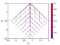
(C) $\varepsilon=5$

(D) $\varepsilon=10$

Figure 1. Steady states for transport activity for perturbation $\varepsilon\mathcal{U}(0,1)$ of the initial transport activity $\overline{X}_{ij}$ with initial data $\overline{X}_{ij},\overline{a}_{i}$.

In Figure 2 we vary the strength $\xi_{S}$ of the source in the top corner of the diamond. As $\xi_{S}$ increases, auxin is transported over a larger area, resulting in lower auxin levels and transport activity close to the source in the top corner of the diamond. Note that the area of large auxin levels and transport activities coincide in the steady states. Further note that not the entire graph is covered with auxin for $\xi_{S}\in\{10,50\}$ and the resulting pattern is symmetric due to symmetric initial data for the auxin levels and the transport activity.

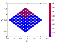
(A) $\xi_{S}=10$

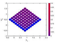
(B) $\xi_{S}=50$

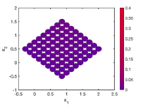
(C) $\xi_{S}=100$

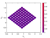
(D) $\xi_{S}=200$

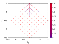
(E) $\xi_{S}=10$

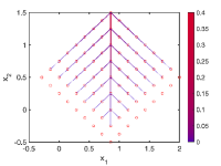
(F) $\xi_{S}=50$

(G) $\xi_{S}=100$

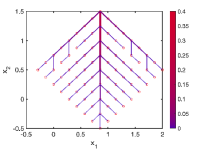
(H) $\xi_{S}=200$

Figure 2. Steady states for auxin concentration and transport activity for different background source strengths $\xi_{S}$ with initial data $\overline{X}_{ij},\overline{a}_{i}$.

In Figure 3 we consider different grids (round, oval). As in Figure 2 we vary the strength $\xi_{S}$ of the source in the top middle corner of these grids. The resulting pattern formation for round and oval grids is very similar to the patterns obtained with the same source strengths in Figure 2 for the diamond grid. In particular, this demonstrates the robustness of the model to variations of the underlying grid. Note that due to the larger size of the oval grid compared to the other considered grids, a stronger source is required for obtaining stationary patterns covering the entire simulation domain.

(A) $\xi_{S}=100$

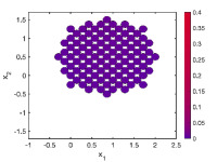
(B) $\xi_{S}=200$

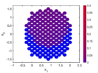
(C) $\xi_{S}=100$

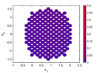
(D) $\xi_{S}=200$

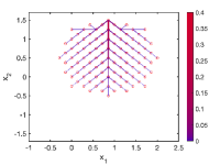
(E) $\xi_{S}=100$

(F) $\xi_{S}=200$

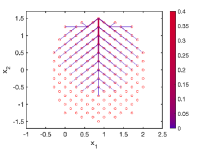
(G) $\xi_{S}=100$

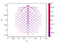
(H) $\xi_{S}=200$

Figure 3. Steady states for auxin concentration and transport activity for different background source strengths $\xi_{S}$ and different grid shapes (round, oval) with initial data $\overline{X}_{ij},\overline{a}_{i}$.

In Figure 4, we vary the strength of the sink in the bottom corner, denoted by $\xi_{I}^{C}$, while keeping the values of $I_{i}$ for all other vertices $i\in V$ as before. Similarly as for the variation of $\xi_{I}$, the area of the network decreases as $\xi_{I}^{C}$ increases for both auxin levels and transport activity. In this case, however, it decreases outside a neighborhood of the line connecting the source in the top corner and the increasing sink of size $\xi_{I}^{C}$ in the bottom corner. In particular, the network structure for large $\xi_{S}^{C}$ is given by a high auxin levels and transport activity along the line of cells, connecting the source in the top corner with the strong sink in the bottom corner. Moreover, this variation of the size of the source $\xi_{S}$ in Figures 2 and 3, as well as, of the sinks $\xi_{I}$ and $\xi_{I}^{C}$ in Figure 4 illustrate how crucial the choice of sources and sinks for the resulting pattern formation is.

(A) $\xi_{I}^{C}=10$

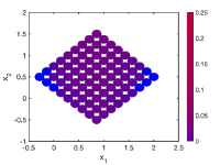
(B) $\xi_{I}^{C}=50$

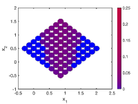
(C) $\xi_{I}^{C}=100$

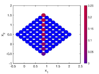
(D) $\xi_{I}^{C}=5000$

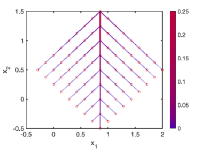
(E) $\xi_{I}^{C}=10$

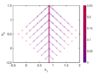
(F) $\xi_{I}^{C}=50$

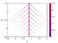
(G) $\xi_{I}^{C}=100$

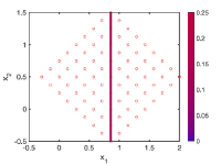
(H) $\xi_{I}^{C}=5000$

Figure 4. Steady states for auxin concentration and transport activity for different sink strengths $\xi_{I}^{C}$ with initial data $\overline{X}_{ij},\overline{a}_{i}$.

In Figures 5 and 6, we investigate the dependence of the stationary states on the model parameters $\delta$ and $\tau$ in (2.9)–(2.10). For small values of $\delta$, more complex stationary patterns for the transport activity can be seen in Figure 5 and auxin is transported over the entire graph. As $\delta$ increases, the auxin levels and the transport activity increase close to the source, but they are no longer transported over the entire graph. As before, the area covered by auxin transport activity and auxin levels are of a similar size, i.e., auxin transport activity and auxin levels are co-existent. The increase of $\tau$ shows a similar change of the steady states of both the auxin transport activity and auxin levels as the increase of $\delta$.

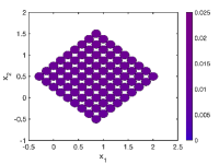
(A) $\delta=0.1$

(B) $\delta=0.5$

(C) $\delta=2$

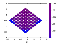
(D) $\delta=10$

(E) $\delta=0.1$

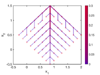
(F) $\delta=0.5$

(G) $\delta=2$

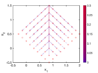
(H) $\delta=10$

Figure 5. Steady states for auxin transport activity and auxin levels for different parameter values $\delta$ with initial data $\overline{X}_{ij},\overline{a}_{i}$.

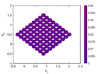
(A) $\tau=0.5$

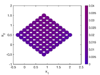
(B) $\tau=2$

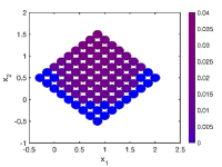
(C) $\tau=5$

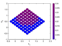
(D) $\tau=10$

(E) $\tau=0.5$

(F) $\tau=2$

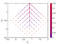
(G) $\tau=5$

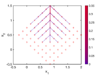
(H) $\tau=10$

Figure 6. Steady states for auxin transport activity and auxin levels for different parameter values $\tau$ with initial data $\overline{X}_{ij},\overline{a}_{i}$.

In Figures 7–9, we vary the initial auxin transport activity and no longer consider the initial data $\overline{X}_{ij}$. In Figure 7, the steady states for the transport activity are shown where the initial transport activity is chosen as $\theta+0.00001\varepsilon$ for parameter $\varepsilon\in\{0.5,5,50,100\}$ and a random variable $\theta$ with $\theta=1$ with probability $0.2$ and $\theta=0$ with probability $0.8$. In particular, the resulting patterns of the transport activity have no symmetries and the location of the mid-veins strongly depend on the choice of parameters, illustrating that model (2.9)–(2.10) can produce complex vein patterns. Note that the size of the stationary pattern increases as $\varepsilon$ and, thus, as the absolute value of the initial transport activity increases.

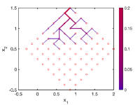
(A) $\varepsilon=0.5$

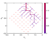
(B) $\varepsilon=5$

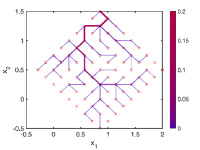
(C) $\varepsilon=50$

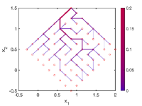
(D) $\varepsilon=100$

Figure 7. Steady states for the transport activity for initial transport activity $\theta+0.00001\varepsilon$ where $\theta$ is a random variable with $\theta=1$ with probability $0.2$ and $\theta=0$ with probability $0.8$.

In Figure 8, we consider the initial transport activity $\varepsilon\mathcal{U}(0,1)$ for $\varepsilon\in\{0.5,1,5,100\}$. These numerical results demonstrate that model (2.9)–(2.10) is capable to produce different complex stationary state, not only on subdomains as in Figure 7, but on the entire underlying network. In particular, the stationary transport activity connects auxin sources and sinks.

(A) $\varepsilon=0.5$

(B) $\varepsilon=1$

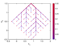
(C) $\varepsilon=5$

(D) $\varepsilon=100$

Figure 8. Steady states for transport activity for initial transport activity $\varepsilon\mathcal{U}(0,1)$.

In Figure 9, we consider the same initial condition for the transport activity as in Figure LABEL:sub@fig:pininitialdatavariation100, i.e. $100\mathcal{U}(0,1)$, but we vary the strengths $10\varepsilon$ and $\varepsilon$ of the auxin background source strengths $\xi_{S}$ and sink strengths $\xi_{I}$, respectively, where $\varepsilon\in\{1,5,50,100\}$. One can clearly see in Figure 9 that the auxin sources and sinks are not strong enough for $\varepsilon=1$ for transport activity to connect the top and bottom corners of the underlying network, while for larger values of $\varepsilon$ mid-veins become visible and get stronger as auxin sources and sinks increase. This shows that complex stationary transport activity patterns with no symmetries and major mid-veins can be obtained.

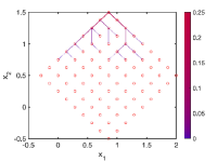
(A) $\varepsilon=1$

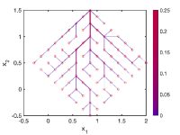
(B) $\varepsilon=5$

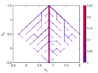
(C) $\varepsilon=50$

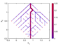
(D) $\varepsilon=100$

Figure 9. Steady states for transport activity for initial transport activity $100\mathcal{U}(0,1)$ with source $10\varepsilon$ and sink $\varepsilon$.

In Figures 10 and 11 we consider multiple sources and sinks for obtaining more realistic vein networks. Starting from a certain configuration of sources and sinks in Figures LABEL:sub@fig:pininitialdatavariationnumbersources1 and LABEL:sub@fig:pininitialdatavariationnumbersourcesrectangle1 we subsequently add sources and sinks in the subfigures further to the right. In Figure 10 we consider a diamond grid as in most figures, but apart from a source at the top corner and a sink at the bottom corner of the grid, we add sources which are located symmetrically with respect to the longest vertical axis of the grid. Denoting the distance between the left and the top corner of grid by $l$, these sources are located on the boundary of the grid at a distance of $l/4$ from the top corner (Figures LABEL:sub@fig:pininitialdatavariationnumbersources1, LABEL:sub@fig:pininitialdatavariationnumbersources2, LABEL:sub@fig:pininitialdatavariationnumbersources3, LABEL:sub@fig:pininitialdatavariationnumbersources4), the left corner (Figures LABEL:sub@fig:pininitialdatavariationnumbersources2, LABEL:sub@fig:pininitialdatavariationnumbersources3, LABEL:sub@fig:pininitialdatavariationnumbersources4) and at distances of $3l/4$ and $5l/8$ from the top corner in Figures LABEL:sub@fig:pininitialdatavariationnumbersources3, LABEL:sub@fig:pininitialdatavariationnumbersources4 and Figure LABEL:sub@fig:pininitialdatavariationnumbersources4, respectively. Similarly, the sources are located on the right side of the grid by symmetry of the source locations in each figure. One can clearly see that multiple sources result in a more complex transportation network between the sources and the sink in comparison to the simulation results in the previous figures with merely one point source.

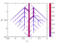
(A) $3$ sources

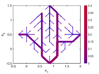
(B) $5$ soures

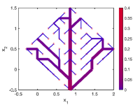
(C) $7$ sources

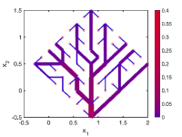
(D) $9$ sources

Figure 10. Steady states for transport activity for initial transport activity $100\mathcal{U}(0,1)$ with different number of sources of strength $1000$ and sinks of strength $100$.

In Figure 11 we consider a rectangular underlying grid with sources at the top and the bottom of the boundary of the grid. We denote the length between the left top and right top corner of the grid by $l$. We consider a sink in the middle of the bottom boundary and sources in the middle of the top boundary and at a distance of $l/4$ left and right of the middle on the top boundary in all subfigures of Figure 11. Additional sources are located at the left top and the right top corner in Figures LABEL:sub@fig:pininitialdatavariationnumbersourcesrectangle2, LABEL:sub@fig:pininitialdatavariationnumbersourcesrectangle3, LABEL:sub@fig:pininitialdatavariationnumbersourcesrectangle4. In Figures LABEL:sub@fig:pininitialdatavariationnumbersourcesrectangle3, LABEL:sub@fig:pininitialdatavariationnumbersourcesrectangle4 additional sinks are added at the bottom boundary in a distance of $l/4$ left and right of the middle of the bottom boundary, while in Figure LABEL:sub@fig:pininitialdatavariationnumbersourcesrectangle4 additional sinks are considered in the left bottom and right bottom corner of the grid. In particular, the resulting patterns look very similar to those in leaves.

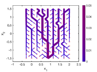
(A) $3$ sources, $1$ sink

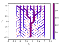
(B) $5$ soures, $1$ sink

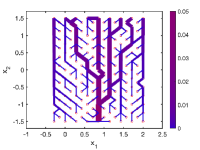
(C) $5$ sources, $3$ sinks

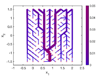
(D) $5$ sources, $5$ sinks

Figure 11. Steady states for transport activity for initial transport activity $100\mathcal{U}(0,1)$ with different number of sources of strength $1000$ and different number of sinks of strength $100$.

Model (2.9)–(2.10) describes the auxin transport with a positive feedback between auxin fluxes and auxin transporters where the auxin transporters are not necessarily polar. The above numerical results illustrate that the model (2.9)–(2.10) is able to connect an auxin source-sink pair with a mid-vein and that branching vein patterns can also be produced. A nice feature of the model is that the veins end up with high auxin levels. This was not achieved with the original Mitchinson models and this has been discussed in some detail. A solution to this has been to adapt the conservative approach $X_{tot}=\sum_{j\in\mathcal{N}(i)}X_{ij}=\text{const}$ for the auxin transporters which (together with feedback on the localisation of auxin transporters from auxin flux) can lead to high auxin in veins.

We want to stress here that our model (2.9)–(2.10) is able to generate a venation/transport network without a polar input, as seen in the case when auxin transporters are knocked out in the various numerical examples.

In reality, the venation patterns appear while the leaf is growing, and as such our simulations (and the simulation results of many previous PIN-based flux models on static geometries) can only provide part of the answer. Changing the configuration of sources and sinks in the model is expected to lead to different patterns in the final leaf.

6. The formal continuum limit

The main reason for focusing on discrete models is that the patterns form when the leaves have very few cells, e.g. the (first) mid-vein forms when the leaf is about five cells wide. Cells split over time, resulting in a larger number of cells and network growth. Besides, there is an auxin peak at the tip before the high auxin/transport activity vein forms downwards from this. Still, this does not discard alternative mechanisms setting up an intitial pattern that connects the leaf tip with the vasculature in the stem (thought to be auxin sink). These phenomena can be modeled much better in a diffusion driven setting instead of the discrete setting and motivates us to consider the associated macroscopic model.

The goal of this section is to derive the formal macroscopic limit of the discrete model (2.10), (2.9) as the number of nodes and edges tends to infinity, and to study the existence of weak solutions of the resulting PDE system. The derivation requires an appropriate rescaling of the auxin production equation (2.9). Moreover, since the derivation of macroscopic limits of systems posed on general (unstructured) graphs is a highly nontrivial topic, see, e.g., [20], we restrict ourselves to discrete graphs represented by regular equidistant grids, i.e., tessellations of a rectangular domain $\Omega\subset\mathbb{R}^{d}$, $d\in\mathbb{N}$, by congruent identical rectangles (in 2D) or cubes (in 3D) with edges parallel to the axis. The results can be generalized to parallelotopes, see [13, Section 3] for details of the formal procedure applied to the Hu-Cai model (2.6)–(2.3), and [12] for the rigorous procedure in the spatially one- and two-dimensional setting.

6.1. The formal derivation of the continuum limit of the system (2.10), (2.9)

Given the graph $G=(V,E)$ as a rectangular tesselation of the rectangular domain $\Omega$, let us denote the vertices left and right of vertex $i\in V$ along the $k$-th spatial dimension by $(i-1)_{k}$ and, resp., $(i+1)_{k}$. Moreover, let us denote $h_{k}>0$ the equidistant grid spacing in the $k$-th dimension. The rescaled auxin production equation (2.9) is then written as

$$\frac{\,\mathrm{d}a_{i}}{\,\mathrm{d}t}=S_{i}-I_{i}a_{i}+\delta\sum_{k=1}^{d}\frac{1}{h_{k}}\left(X_{i,(i+1)_{k}}\frac{a_{(i+1)_{k}}-a_{i}}{h_{k}}-X_{i,(i-1)_{k}}\frac{a_{i}-a_{(i-1)_{k}}}{h_{k}}\right)\qquad\text{for~{}}i\in V.$$ (6.1)

The rescaling of the sum on the right hand side by $h_{k}$ is reflecting the fact that the edges of the graph are inherently one-dimensional structures, embedded into the $d$-dimensional space, cf. [13, Section 3]. A straightforward calculation reveals that (6.1) is a finite difference discretization of the parabolic equation

$$\frac{\partial a}{\partial t}=\delta\nabla\cdot(X\nabla a)+S-Ia,$$ (6.2)

on the regular grid $G=(V,E)$, where $a=a(t,x)$ is a formal limit of the sequence of discrete auxin concentrations $(a_{i})_{i\in V}$ as $|V|\to\infty$, and $I=I(x)$ is a formal limit of the sequence $(I_{i})_{i\in V}$. Here, $X=X(t,x)$ is the diagonal tensor $X=\text{diag}(X_{1},\ldots,X_{d})$ where $X_{k}$ is the formal limit of the sequence $(X_{ij})_{i,j\in V}$ on edges $(i,j)\in E$ oriented along the $k$-th spatial direction. A formal continuum limit of (2.10) yields the family of ODEs for $X=X(t,x)$,

$$\frac{\partial X_{k}}{\partial t}=\left(\frac{|q_{k}|^{\kappa}}{X_{k}^{\gamma+1}}-\tau\right)X_{k},$$ (6.3)

with $q_{k}=X_{k}\partial_{x_{k}}a$. Note that the product $X\nabla a$ is the vector $X\nabla a=(X_{1}\partial_{x_{1}}a,\dots,X_{d}\partial_{x_{d}}a)$.

Observe that (6.3) is in fact a family of ODEs for $X_{k}=X_{k}(t,x)$, parametrized by $x\in\Omega$. Consequently, in analogy to [13], we introduce the diffusive terms $D^{2}\Delta X_{k}$ that model random fluctuations in the medium. Thus, the updated version of (6.3) reads

$$\frac{\partial X_{k}}{\partial t}=D^{2}\Delta X_{k}+\left(\frac{|q_{k}|^{\kappa}}{X_{k}^{\gamma+1}}-\tau\right)X_{k},$$ (6.4)

with the diffusion coefficient $D^{2}>0$.

Biological observations suggest that the auxin dynamics takes place on a faster time scale than the dynamics of the transporter proteins in the order of minutes for auxin movement [7], and in the order of hours for e.g. PIN1 reorientation [14]. Consequently, we consider a formal fast time scale limit of (6.2), assuming large $\delta$, $S$ and $I$, which leads to the elliptic equation

$$-\delta\nabla\cdot(X\nabla a)=S-Ia.$$ (6.5)

The system (6.2), (6.4) is equipped with the no-flux boundary condition

$$\nu\cdot X\nabla a=0,\qquad\nu\cdot\nabla X_{k}=0\qquad\mbox{on }\partial\Omega,\,k=1,\dots,d,$$ (6.6)

where $\nu=\nu(x)$ is the outer unit normal vector on $\partial\Omega$. The no-flux boundary condition reflects the modeling assumption that there is no flow of auxin or the auxin transporters through the boundary of the domain. More general boundary conditions can be considered, leading to only slight modifications in the forthcoming analysis. Moreover, we prescribe the initial datum for the auxin transporters

$$X_{k}(0,x)=X_{k}^{0}(x)\geq 0\qquad\mbox{for }x\in\Omega,\,k=1,\dots,d.$$ (6.7)

Remark 1.

The choice to work with the elliptic-parabolic system (6.4), (6.5) instead of the parabolic-parabolic system (6.2), (6.4) simplifies the mathematical analysis, since one can apply the so-called weak-strong lemma for the elliptic equation (6.5), see Lemma 2 below. The analysis of the full parabolic-parabolic PDE system (6.2), (6.4) will be the subject of a further work.

6.2. Existence of weak solutions for the system (6.4), (6.5)

The weak formulation of (6.5), subject to the no-flux boundary condition (6.6), with a test function $\phi\in C^{\infty}(\Omega)$ reads

$$\delta\int_{\Omega}(X\nabla a)\cdot\nabla\phi\,\mathrm{d}x=\int_{\Omega}(S-Ia)\phi\,\mathrm{d}x,$$ (6.8)

for almost all $t>0$, and the weak formulation of (6.4), (6.6) with a test function $\psi\in C^{\infty}(\Omega)$ is

$$\frac{\,\mathrm{d}}{\,\mathrm{d}t}\int_{\Omega}{X_{k}}\psi\,\mathrm{d}x=-D^{2}\int_{\Omega}\nabla X_{k}\cdot\nabla\psi\,\mathrm{d}x+\int_{\Omega}\left({|\partial_{x_{k}}a|^{\kappa}}{X_{k}^{\kappa-\gamma}}-\tau X_{k}\right)\psi\,\mathrm{d}x,$$ (6.9)

for almost all $t>0$. The system is subject to the initial datum (6.7) with

$$X_{k}^{0}\in L^{\infty}(\Omega),\quad k=1,\dots,d.$$ (6.10)

We assume the uniform positivity $X_{k}^{0}\geq\overline{X}^{0}>0$ almost everywhere on $\Omega$, which prevents degeneracy of the elliptic term $\nabla\cdot(X\nabla a)$ in (6.2). Moreover, we assume that

$$S\in L^{2}(\Omega),\qquad I\in L^{\infty}(\Omega)\text{ with }I(x)\geq\overline{I}>0\text{ almost everywhere on }\Omega.$$ (6.11)

To prove the existence of solutions of the system (6.8), (6.9) subject to the initial condition (6.10) we shall use the Schauder fixed point iteration in an appropriate function space. We start by proving suitable a-priori estimates.

Lemma 1.

Let $S\in L^{2}(\Omega)$ and $I\in L^{\infty}(\Omega)$ verify (6.11). Let the diagonal tensor $X\in L^{2}(\Omega)$ be uniformly positive on $\Omega$, i.e., let there be $\overline{X}>0$ such that $X_{k}\geq\overline{X}$ almost everywhere on $\Omega$, for $k=1,\dots,d$. Then there exists a unique solution $a\in H^{1}(\Omega)$ of (6.8) and a constant $C>0$ depending only $\delta$, $\overline{X}$, $S$ and $\overline{I}$, such that

$$\left\|a\right\|_{H^{1}(\Omega)}\leq C.$$ (6.12)

Proof.

Let us consider a sequence of uniformly positive diagonal tensors $X^{n}\in L^{\infty}((0,T)\times\Omega)$, $X^{n}_{k}\geq\overline{X}$ almost everywhere on $\Omega$ for all $n\in\mathbb{N}$, such that $X^{n}\to X$ in the norm topology of $L^{2}((0,T)\times\Omega)$ as $n\to\infty$. For each $n\in\mathbb{N}$ a unique solution $a^{n}\in H^{1}(\Omega)$ of (6.8) is constructed using the Lax-Milgram Theorem, see, e.g., [9]. The continuity of the bilinear form $B:H^{1}(\Omega)\times H^{1}(\Omega)\to\mathbb{R}$ associated with (6.8),

$$B(a,\phi):=\delta\int_{\Omega}(X\nabla a)\cdot\nabla\phi\,\mathrm{d}x-\int_{\Omega}(S-Ia)\phi\,\mathrm{d}x,$$

follows from a straightforward application of the Cauchy-Schwart inequality. The coercivity of $B$ follows from

$$-\int_{\Omega}Sa\,\mathrm{d}x\geq-\frac{1}{4\overline{I}}\int_{\Omega}S^{2}\,\mathrm{d}x-\overline{I}\int_{\Omega}a^{2}\,\mathrm{d}x$$

and the uniform boundedness $I(x)\geq\overline{I}$. Using $\phi:=a^{n}$ as a test function in (6.8) gives

$$\delta\int_{\Omega}\nabla a^{n}\cdot X^{n}\nabla a^{n}\,\mathrm{d}x=\int_{\Omega}Sa^{n}\,\mathrm{d}x-\int_{\Omega}I(a^{n})^{2}\,\mathrm{d}x,$$

By (6.11), the Cauchy-Schwartz inequality and the uniform boundedness $X^{n}_{k}\geq\overline{X}>0$ we have

$$\delta\overline{X}\int_{\Omega}|\nabla a^{n}|^{2}\,\mathrm{d}x+\frac{\overline{I}}{2}\int_{\Omega}(a^{n})^{2}\,\mathrm{d}x\leq\frac{1}{2\overline{I}}\int_{\Omega}S^{2}\,\mathrm{d}x$$ (6.13)

and thus a uniform bound on $a^{n}$ in $H^{1}(\Omega)$.

Consequently, we can extract a subsequence converging to some $a$ weakly in $H^{1}(\Omega)$ and strongly in $L^{2}(\Omega)$. Then, it is trivial to pass to the limit in (6.8), where the term $X^{n}\nabla a^{n}$ converges to $X\nabla a$ due to the strong convergence of $X^{n}$ in $L^{2}(\Omega)$. Consequently, the limiting object $a$ verifies the weak formulation (6.8). Moreover, it satisfies the a-priori estimates (6.13) due to the weak lower semicontinuity of the respective norms. Uniqueness of the solution follows from (6.13) and the linearity of the equation.

 

Remark 2.

With a straightforward modification of its proof, we shall apply Lemma 1 for time-dependent permeability tensors $X\in L^{\infty}(0,T;L^{2}(\Omega))$ in the sequel. We then obtain the unique solution $a\in L^{2}(0,T;H^{1}(\Omega))$ satisfying the uniform estimate

$$\left\|a\right\|_{L^{2}(0,T;H^{1}(\Omega))}\leq C$$ (6.14)

with $C=C(\delta,\overline{X},S,\overline{I})>0$.

The following Lemma is an instance of the so-called weak-strong lemma for elliptic problems, see, e.g. [12, Lemma 1]. Here we formulate it in the time-dependent setting with $a=a(t,x)$.

Lemma 2.

Fix $T>0$ and let $(X^{n})_{n\in\mathbb{N}}\subset L^{\infty}(0,T;L^{2}(\Omega))$ be a sequence of diagonal tensors in $\mathbb{R}^{d\times d}$ such that for some $\overline{X}>0$, $X^{n}_{k}\geq\overline{X}>0$ almost everywhere on $(0,T)\times\Omega$, $k=1,\dots,d$, $n\in\mathbb{N}$. Moreover, assume that $X^{n}\to X$ in the norm topology of $L^{2}((0,T)\times\Omega)$. Let $(a^{n})_{n\in\mathbb{N}}$ be a sequence of weak solutions of (6.8) with the permeability tensors $X^{n}$. Then $\nabla a^{n}$ converges to $\nabla a$ strongly in $L^{q}((0,T)\times\Omega)$ for any $q<2$, where $a$ is the solution of (6.8) with permeability tensor $X$.

Proof.

Due to the uniform estimate on $a^{n}$ in $L^{2}(0,T;H^{1}(\Omega))$ of Lemma 1, $a^{n}$ that converges weakly in $L^{2}(0,T;H^{1}(\Omega))$ to some $a$. Since $a^{n}\to a$ strongly in $L^{2}((0,T)\times\Omega)$, we can pass to the limit $n\to\infty$ in (6.8). With the uniform estimate on $\sqrt{X^{n}}\nabla a^{n}$ in $L^{2}((0,T)\times\Omega)$ provided by (6.14), the weak lower semicontinuity of the $L^{2}$-norm implies

$$\int_{0}^{T}\int_{\Omega}X\nabla a\cdot\nabla a\,\mathrm{d}x\,\mathrm{d}t=\int_{0}^{T}\int_{\Omega}|\sqrt{X}\nabla a|^{2}\,\mathrm{d}x\,\mathrm{d}t\leq\liminf_{n\to\infty}\int_{0}^{T}\int_{\Omega}|\sqrt{X^{n}}\nabla a^{n}|^{2}\,\mathrm{d}x\,\mathrm{d}t<+\infty$$ (6.15)

for almost all $t>0$. Consequently, we can use $a$ as a test function in the time-integrated version of (6.8) to obtain

$$\delta\int_{0}^{T}\int_{\Omega}X\nabla a\cdot\nabla a\,\mathrm{d}x\,\mathrm{d}t=\int_{0}^{T}\int_{\Omega}(S-Ia)a\,\mathrm{d}x\,\mathrm{d}t.$$

Then, using $a^{N}$ as a test function in (6.8) with $X^{n}$, we have

$$\lim_{N\to\infty}\delta\int_{0}^{T}\int_{\Omega}X^{n}\nabla a^{n}\cdot\nabla a^{n}\,\mathrm{d}x=\int_{0}^{T}\int_{\Omega}(S-Ia)a\,\mathrm{d}x\,\mathrm{d}t=\delta\int_{0}^{T}\int_{\Omega}X\nabla a\cdot\nabla a\,\mathrm{d}x\,\mathrm{d}t.$$

Consequently,

$$\int_{0}^{T}\int_{\Omega}|\sqrt{X}\nabla a|^{2}\,\mathrm{d}x\,\mathrm{d}t=\lim_{n\to\infty}\int_{0}^{T}\int_{\Omega}|\sqrt{X^{n}}\nabla a^{n}|^{2}\,\mathrm{d}x\,\mathrm{d}t,$$

so that we have the strong convergence of $\sqrt{X^{n}}\nabla a^{n}$ to $\sqrt{X}\nabla a$ in $L^{2}((0,T)\times\Omega)$. Now we write,

$$\int_{0}^{T}\int_{\Omega}|\partial_{x_{k}}a^{n}-\partial_{x_{k}}a|\,\mathrm{d}x\,\mathrm{d}t \leq\overline{X}^{-1/2}\int_{0}^{T}\int_{\Omega}|\sqrt{X_{k}}\partial_{x_{k}}a^{n}-\sqrt{X_{k}}\partial_{x_{k}}a|\,\mathrm{d}x\,\mathrm{d}t$$

$$\leq\overline{X}^{-1/2}\left\|\nabla a^{n}\right\|_{L^{2}((0,T)\times\Omega)}\left\|\sqrt{X_{k}^{n}}-\sqrt{X_{k}}\right\|_{L^{2}((0,T)\times\Omega)}$$

$$\quad+\overline{X}^{-1/2}\int_{0}^{T}\int_{\Omega}|\sqrt{X^{n}_{k}}\partial_{x_{k}}a^{n}-\sqrt{X_{k}}\partial_{x_{k}}a|\,\mathrm{d}x\,\mathrm{d}t,$$

for $k=1,\dots,d$, and the first term of the right-hand side converges to zero due to the assumed strong convergence of $X^{n}$ in $L^{2}((0,T)\times\Omega)$, while the second term does so due to the strong convergence of $\sqrt{X^{n}}\nabla a^{n}$. Thus, we have the strong convergence of $\nabla a^{n}$ to $\nabla a$ in $L^{1}((0,T)\times\Omega)$. Since $\nabla a^{n}$ is also uniformly bounded in $L^{2}((0,T)\times\Omega)$, a simple consequence of the interpolation inequality [28, Chapter 1] implies strong convergence in $L^{q}((0,T)\times\Omega)$ for $q<2$.

 

Lemma 3.

Fix $T>0$ and let $\nabla a\in L^{2}((0,T)\times\Omega)$. Let $\kappa>\gamma$ and,

$$\kappa<2\quad\mbox{for }d\in\{1,2\},\qquad\kappa\leq\frac{\gamma+5}{4}\quad\mbox{for }d=3,$$ (6.16)

depending on the space dimension $d$. Then there exists a unique solution

$$X_{k}\in L^{2}(0,T;H^{1}(\Omega))\cap L^{\infty}(0,T;L^{2}(\Omega))\cap C([0,T);H^{-1}(\Omega)),\qquad k=1,\dots,d,$$

of (6.9) subject to the initial datum (6.10) with $X_{k}^{0}\geq\overline{X}^{0}>0$ almost everywhere on $\Omega$. Moreover, the solution stays uniformly bounded away from zero on $(0,T)\times\Omega$, i.e., there exists $\overline{X}>0$ depending on $\overline{X}^{0}$, $T$, $D^{2}$ and $\tau$, but independent of $a$, such that

$$X_{k}\geq\overline{X}>0\qquad\mbox{almost everywhere on }(0,T)\times\Omega.$$ (6.17)

Moreover, there exists a constant $K_{0}>0$ independent of $X$ and $a$ such that

$$\left\|X_{k}\right\|^{2}_{L^{\infty}(0,T;L^{2}(\Omega))}\leq\left\|X_{k}^{0}\right\|_{L^{2}(\Omega)}^{2}+K_{0}\left\|\partial_{x_{k}}a\right\|_{L^{2}((0,T)\times\Omega)}^{2}$$ (6.18)

and, for $k=1,\dots,d$,

$$\left\|\nabla X_{k}\right\|^{2}_{L^{2}(0,T;L^{2}(\Omega))}\leq\left\|X_{k}^{0}\right\|_{L^{2}(\Omega)}^{2}+K_{0}\left\|\partial_{x_{k}}a\right\|_{L^{2}((0,T)\times\Omega)}^{2}.$$ (6.19)

Remark 3.

Observe that the necessary condition for the mutual validity of the assumptions $\kappa>\gamma$ and (6.16) is $\gamma,\kappa<2$ for $d\in\{1,2\}$ and $\gamma,\kappa\leq 5/3$ for $d=3$.

Proof.

Let us fix $k\in\{1,\dots,d\}$ and use $\psi:=X_{k}$ as a test function in (6.9),

$$\frac{1}{2}\frac{\,\mathrm{d}}{\,\mathrm{d}t}\int_{\Omega}X_{k}^{2}\,\mathrm{d}x=-D^{2}\int_{\Omega}|\nabla X_{k}|^{2}\,\mathrm{d}x+\int_{\Omega}|\partial_{x_{k}}a|^{\kappa}X_{k}^{\kappa-\gamma+1}\,\mathrm{d}x-\tau\int_{\Omega}X_{k}^{2}\,\mathrm{d}x,$$ (6.20)

where we used the identity $q_{k}=X_{k}\partial_{x_{k}}a$. Using the Hölder inequality with exponents $p$ and $p^{\prime}$, $\frac{1}{p}+\frac{1}{p^{\prime}}=1$, we have

$$\int_{\Omega}|\partial_{x_{k}}a|^{\kappa}X_{k}^{\kappa-\gamma+1}\,\mathrm{d}x\leq C_{\varepsilon}\int_{\Omega}|\partial_{x_{k}}a|^{\kappa p}\,\mathrm{d}x+\varepsilon\int_{\Omega}|X_{k}|^{(\kappa-\gamma+1)p^{\prime}}\,\mathrm{d}x$$ (6.21)

for $\varepsilon>0$ and a suitable constant $C_{\varepsilon}$. Due to the assumed $L^{2}$-integrability of $\partial_{x_{k}}a$, we choose $\kappa p=2$, so that $p^{\prime}=\frac{2}{2-\kappa}$. Denote $\alpha:=(\kappa-\gamma+1)p^{\prime}$ and observe that $\alpha>0$ due to the assumption $\kappa>\gamma$. Let us distinguish the following two cases: If $\alpha\leq 2$, then by the Hölder inequality we have

$$\int_{\Omega}|X_{k}|^{\alpha}\,\mathrm{d}x\leq C_{\Omega}\int_{\Omega}|X_{k}|^{2}\,\mathrm{d}x,$$

so that (6.20) and (6.21) imply

$$\frac{1}{2}\frac{\,\mathrm{d}}{\,\mathrm{d}t}\int_{\Omega}X_{k}^{2}\,\mathrm{d}x\leq-D^{2}\int_{\Omega}|\nabla X_{k}|^{2}\,\mathrm{d}x+C_{\varepsilon}\int_{\Omega}|\partial_{x_{k}}a|^{2}\,\mathrm{d}x-(\tau-\varepsilon C_{\Omega})\int_{\Omega}X_{k}^{2}\,\mathrm{d}x,$$

and choosing $\varepsilon>0$ such that $\tau-\varepsilon C_{\Omega}>0$ directly implies the a-priori estimates (6.18) and (6.19). On the other hand, if $\alpha>2$, we apply the Sobolev inequality [9]

$$\int_{\Omega}|X_{k}|^{\alpha}\,\mathrm{d}x\leq C_{S}\left(\int_{\Omega}|\nabla X_{k}|^{2}\,\mathrm{d}x+\int_{\Omega}|X_{k}|^{2}\,\mathrm{d}x\right)$$

with $C_{S}=C_{S}(\Omega)$ the Sobolev constant. Depending on the space dimension, we have:

• For $d\in\{1,2\}$,

  $$\left\|X_{k}\right\|_{L^{\alpha}(\Omega)}\leq C_{S}\left(\int_{\Omega}|\nabla X_{k}|^{2}\,\mathrm{d}x+\int_{\Omega}|X_{k}|^{2}\,\mathrm{d}x\right)$$ (6.22)

  for any $\alpha<\infty$, i.e., we admit any $p>1$ and, consequently, $\kappa<2$.

• For $d=3$ we have (6.22) for $\alpha\leq 6$, i.e., we need $(\kappa-\gamma+1)p^{\prime}=\frac{2(\kappa-\gamma+1)}{2-\kappa}\leq 6$, which gives the condition $\kappa\leq\frac{\gamma+5}{4}$.

Consequently, we have

$$\frac{1}{2}\frac{\,\mathrm{d}}{\,\mathrm{d}t}\int_{\Omega}X_{k}^{2}\,\mathrm{d}x\leq-(D^{2}-\varepsilon C_{S})\int_{\Omega}|\nabla X_{k}|^{2}\,\mathrm{d}x+C_{\varepsilon}\int_{\Omega}|\partial_{x_{k}}a|^{2}\,\mathrm{d}x-(\tau-\varepsilon C_{S})\int_{\Omega}X_{k}^{2}\,\mathrm{d}x,$$

and choosing $\varepsilon>0$ such that $\varepsilon C_{S}<\min\{D^{2},\tau\}$ directly implies the a-priori estimates (6.18) and (6.19). The uniform positivity (6.17) follows from the fact that solutions $u=u(t,x)$ of the linear parabolic equation $\frac{\partial u}{\partial t}=D^{2}\Delta u-\tau u$ are subsolutions to (6.3), and they remain uniformly positive on bounded time intervals for uniformly positive initial data, see, e.g., [9].

Finally, note that we have the identity (in distributional sense)

$$\frac{\partial X_{k}}{\partial t}=D^{2}\Delta X_{k}+|\partial_{x_{k}}a|^{\kappa}X_{k}^{\kappa-\gamma}-\tau X_{k}.$$

An easy calculation reveals that, for the aforementioned range of $\kappa$ and $\gamma$,

$$|\partial_{x_{k}}a|^{\kappa}X_{k}^{\kappa-\gamma}\in L^{1}(0,T;L^{6/5}(\Omega))\subset L^{1}(0,T;H^{-1}(\Omega)),$$

implying $\frac{\partial X_{k}}{\partial t}\in L^{1}(0,T;H^{-1}(\Omega))$, so that $X_{k}\in C([0,T);H^{-1}(\Omega))$, see, e.g., [28, Chapter 7].

 

Theorem 2.

Fix $T>0$ and let $\kappa>\gamma$, and, in dependence of the space dimension $d$,

$$\begin{aligned} \kappa&<\frac{\gamma+4}{3}\quad\mbox{for }d\in\{1,2\},\qquad\kappa&<\frac{\gamma+5}{4}\quad\mbox{for }d=3.\end{aligned}$$ (6.23)

Then the system (6.8)–(6.9) subject to the initial datum (6.10) with $X_{k}^{0}\geq\overline{X}^{0}>0$ almost everywhere on $\Omega$ admits a weak solution $(X,a)$ on $(0,T)$ such that

$$\begin{aligned} X_{k}&\in L^{\infty}(0,T;L^{2}(\Omega))\cap L^{2}(0,T;H^{1}(\Omega))\cap C([0,T);H^{-1}(\Omega)),\\ a&\in L^{\infty}(0,T;L^{2}(\Omega))\cap L^{2}(0,T;H^{1}(\Omega))\cap C([0,T);W^{-1,4/3}(\Omega)).\end{aligned}$$ (6.24)

Proof.

We construct a solution using the Schauder fix-point theorem on the set

$$\mathcal{B}_{T}:=\Bigl{\{}X\in(L^{\infty}(0,T;L^{2}(\Omega)))^{d\times d}_{\mathrm{diag}};\;\left\|X_{k}\right\|^{2}_{L^{\infty}(0,T;L^{2}(\Omega))}\leq\left\|X_{k}^{0}\right\|_{L^{2}(\Omega)}^{2}+K_{0}B_{T}^{2},\;$$

$$X_{k}\geq\overline{X}\mbox{ almost everywhere on }(0,T)\times\Omega,\;k=1,\dots,d\Bigr{\}}.$$

Here $(L^{\infty}(0,T;L^{2}(\Omega)))^{d\times d}_{\mathrm{diag}}$ denotes the space of diagonal $d\times d$-tensors with entries in $L^{\infty}(0,T;L^{2}(\Omega))$, and $K_{0}$ and $\overline{X}$ are the constant defined in Lemma 3; note that they depend only on $\overline{X}^{0}$, $T$, and the parameters $\kappa$, $\gamma$, $D^{2}$ and $\tau$. Moreover, we denoted

$$B^{2}_{T}:=\frac{1}{2\delta\overline{X}}\left((Te^{T}+1)\left\|a^{0}\right\|_{L^{2}(\Omega)}^{2}+Te^{T}\left\|S\right\|_{L^{2}(\Omega)}^{2}\right).$$

The set $\mathcal{B}_{T}$ shall be equipped with the norm topology of $L^{2}((0,T)\times\Omega)$. Obviously, $\mathcal{B}_{T}$ is nonempty, convex and closed. We define the mapping $\Phi:\mathcal{B}_{T}\to L^{\infty}(0,T;L^{2}(\Omega))$,

$$\Phi:X\in\mathcal{B}_{T}\mapsto\tilde{X},$$ (6.25)

where given $X\in\mathcal{B}_{T}$ we construct $a$ the unique weak solution of (6.8) by Lemma 1, and, subsequently, construct $\tilde{X}$ as the unique weak solution of (6.9) by Lemma 3. Clearly, due to the a-priori estimates (6.12) and (6.18), $\tilde{X}\in\mathcal{B}_{T}$.

To prove the continuity of the mapping $\Phi$, let us consider a sequence $(X_{n})_{n\in\mathbb{N}}\subset\mathcal{B}_{T}$, converging to $X\in\mathcal{B}_{T}$ in the norm topology of $L^{2}((0,T)\times\Omega)$. Denote $(a_{n})_{n\in\mathbb{N}}$ and, resp., $a$, the solutions of (6.8) corresponding to $X_{n}$ and, resp., $X$. Then, due to Lemma 2, $\nabla a_{n}$ converges to $\nabla a$ in the norm topology of $L^{q}((0,T)\times\Omega)$ for any $q<2$. Let $\tilde{X}_{n}:=\Phi(X_{n})$ and $\tilde{X}:=\Phi(X)$. Due to Lemma 3 and the Aubin-Lions theorem, a subsequence of $\tilde{X}_{n}$ converges strongly to some $\tilde{X}^{*}$ in $L^{2}(0,T;L^{q}(\Omega))$ with $q<\infty$ if $d\in\{1,2\}$ and $q=6$ if $d=3$. The limit passage $n\to\infty$ in (6.9) is trivial for the linear terms. For the term $|\partial_{x_{k}}a_{n}|^{\kappa}\tilde{X}_{n}^{\kappa-\gamma}$ we observe that, due to Lemma 2, the term $|\partial_{x_{k}}a_{n}|^{\kappa}$ converges to $|\partial_{x_{k}}a|^{\kappa}$ in the norm topology of $L^{q}((0,T)\times\Omega)$ for $q<{2}/{\kappa}$. Moreover:

• For $d\in\{1,2\}$, the interpolation inequality between $L^{\infty}(0,T;L^{2}(\Omega))$ and $L^{2}(0,T;L^{q}(\Omega))$ with $q<\infty$ implies that $\tilde{X}^{n}$ is uniformly bounded, and thus converges, in the norm topology of $L^{q}((0,T)\times\Omega)$ for $q<4$. Consequently, since $\kappa<2$, the product $|\partial_{x_{k}}a_{n}|^{\kappa}\tilde{X}_{n}^{\kappa-\gamma}$ converges strongly in (at least) $L^{1}((0,T)\times\Omega)$ to $|\partial_{x_{k}}a|^{\kappa}(\tilde{X}^{*}_{n})^{\kappa-\gamma}$ if $\frac{\kappa}{2}+\frac{\kappa-\gamma}{4}<1$, which is equivalent to $\kappa<\frac{\gamma+4}{3}$.

• For $d=3$ the interpolation inequality between $L^{\infty}(0,T;L^{2}(\Omega)$ and $L^{2}(0,T;L^{6}(\Omega))$ implies that $\tilde{X}^{n}$ is uniformly bounded in the norm topology of $L^{10/3}((0,T)\times\Omega)$. Then the sufficient condition for $L^{1}$-convergence of the product $|\partial_{x_{k}}a_{n}|^{\kappa}\tilde{X}_{n}^{\kappa-\gamma}$ reads $\frac{\kappa}{2}+\frac{3(\kappa-\gamma)}{10}<1$, which is equivalent to $\kappa<\frac{10+3\gamma}{8}$. This condition is weaker than (6.23).

By the uniqueness of solutions of (6.8), we conclude that $\tilde{X}^{*}=\tilde{X}$, i.e., the mapping $\Phi$ is continuous on $\mathcal{B}_{T}$ with respect to the norm topology of $L^{2}((0,T)\times\Omega)$.

To prove the compactness of the mapping $\Phi$, we employ the Aubin-Lions lemma [3]. Let us again consider a sequence $(X_{n})_{n\in\mathbb{N}}\subset\mathcal{B}_{T}$ and denote $\tilde{X}_{n}:=\Phi(X_{n})$. Due to the a-priori estimates (6.12) and (6.18), (6.19), the sequence $\tilde{X}_{n}$ is bounded in $L^{\infty}(0,T;L^{2}(\Omega))$ and in $L^{2}(0,T;H^{1}(\Omega))$. Moreover, $\partial_{t}\tilde{X}_{n}$ is bounded in $L^{1}(0,T;H^{-1}(\Omega))$. Then, since $H^{1}(\Omega)$ is compactly embedded into $L^{2}(\Omega)$ and $L^{2}(\Omega)\subset H^{-1}(\Omega)$, the Aubin-Lions theorem provides the relative compactness of the sequence $\tilde{X}_{n}$ with respect to the norm topology of $L^{2}((0,T)\times\Omega))$. Consequently, the Schauder fix-point theorem provides a solution $(X,a)$ of the system (6.8)–(6.10), satisfying (6.24).

 

Remark 4.

For the case $\kappa=\gamma=2$ the system (6.4) simplifies to

$$\frac{\partial X_{k}}{\partial t}=D^{2}\Delta X_{k}+{(\partial_{x_{k}}a)^{2}}-\tau X_{k}.$$ (6.26)

Then, (6.5), (6.26) is similar to the system studied in [13] and [12], the main difference being that the permeability tensor in the elliptic equation is of the form $rI+X$ in [13], [12], where $r>0$ is a constant. The significant property of (6.5), (6.26) is its energy-dissipation structure. Indeed, defining

$$\mathcal{E}[X]:=\frac{D^{2}}{2}\sum_{k=1}^{d}\int_{\Omega}|\nabla X_{k}|^{2}\,\mathrm{d}x+\int_{\Omega}\nabla a\cdot X\nabla a\,\mathrm{d}x+\tau\sum_{k=1}^{d}\int_{\Omega}X_{k}^{2}\,\mathrm{d}x,$$

where $a=a[X]$ is the unique weak solution of (6.5), a simple calculation (see [13, Lemma 3]) reveals that,

$$\frac{\,\mathrm{d}}{\,\mathrm{d}t}\mathcal{E}[X]=-\sum_{k=1}^{d}\int_{\Omega}\left(\frac{\partial X_{k}}{\partial t}\right)^{2}\,\mathrm{d}x$$

along the solutions of (6.5), (6.26). The energy dissipation naturally provides uniform a-priori estimates on $X$ and $a$ in the energy space. However, these still do not allow us to extend the validity of Theorem 2 to $\kappa=\gamma=2$. The problem is that in the proof of continuity of the fix-point mapping $\Phi$, it is not clear how to pass to the (weak) limit in the sequence $(\partial_{x_{k}}a)^{2}$. Note that Lemma 2 only provides (strong) convergence of $\partial_{x_{k}}a$ in $L^{q}((0,T)\times\Omega)$ with $q<2$.

Remark 5 (Steady states of the system (6.4), (6.5) with $D^{2}=0$).

The steady states of the system (6.4), (6.5) with $D^{2}=0$ satisfy, in the weak sense,

$$\delta\nabla\cdot(X\nabla a)+S-Ia=0,$$ (6.27)

$$|\partial_{x_{k}}a|^{\kappa}X_{k}^{\kappa-\gamma}-\tau X_{k}=0,$$ (6.28)

for $k=1,\dots,d$, with $q_{k}=X_{k}\partial_{x_{k}}a$. For $\kappa>\gamma>0$, (6.28) implies that there exist measurable sets $\mathcal{A}_{k}\subset\Omega$, $k=1,\dots,d$, such that

$$X_{k}=\left(\frac{|\partial_{x_{k}}a|^{\kappa}}{\tau}\right)^{\frac{1}{\gamma-\kappa+1}}\chi_{k},$$

where $\chi_{k}=\chi_{k}(x)$ is the characteristic function of $\mathcal{A}_{k}$. Inserting this into (6.27), we obtain

$$-\delta\tau^{\frac{1}{\kappa-\gamma-1}}\sum_{k=1}^{d}\partial_{x_{k}}\left(\chi_{k}|\partial_{x_{k}}a|^{\frac{\kappa}{\gamma-\kappa+1}}\partial_{x_{k}}a\right)=S-Ia.$$ (6.29)

Due to the presence of the characteristic functions $\chi_{k}$, this is a strongly degenerate elliptic equation, rendering its analysis a very challenging task, which we leave for a future work. Let us only note that the degeneracy in (6.29) induces strong nonuniqueness of its solutions. Consequently, it is necessary to equip (6.29) with suitable selection criteria in order to obtain unique solutions. This is to be done through further modeling inputs. For $\kappa=\gamma>0$, contrarily, (6.28) gives $X_{k}=\tau^{-1}|\partial_{x_{k}}a|^{\kappa}$, and (6.27) reads

$$-\delta\tau^{-1}\sum_{k=1}^{d}\partial_{x_{k}}\left(|\partial_{x_{k}}a|^{\kappa}\partial_{x_{k}}a\right)=S-Ia.$$ (6.30)

Equipped with the no-flux boundary condition (6.6), its weak formulation reads

$$\delta\tau^{-1}\sum_{k=1}^{d}\int_{\Omega}|\partial_{x_{k}}a|^{\kappa}(\partial_{x_{k}}a)(\partial_{x_{k}}\psi)\,\mathrm{d}x+\int_{\Omega}(a-S)\psi\,\mathrm{d}x=0$$ (6.31)

for all test functions $\psi\in C^{\infty}(\Omega)$. Weak solutions $a\in W^{1,\kappa+2}(\Omega)$ of (6.31) are constructed as the global minima of the functional $\mathcal{F}:W^{1,\kappa+2}\to\mathbb{R}$,

$$\mathcal{F}[a]:=\frac{\delta\tau^{-1}}{\kappa+2}\sum_{k=1}^{d}\int_{\Omega}|\partial_{x_{k}}a|^{\kappa+2}\,\mathrm{d}x+\frac{1}{2}\int_{\Omega}a^{2}\,\mathrm{d}x-\int_{\Omega}Sa\,\mathrm{d}x.$$

Obviously, for $\kappa>0$ the functional is uniformly convex. Moreover, a straightforward application of the Cauchy-Schwartz inequality implies boundedness below and coercivity of $\mathcal{F}$ with respect to the norm of $W^{1,\kappa+2}(\Omega)$. Then the classical theory (see, e.g., [9]) provides the existence of a unique minimizer $a\in W^{1,\kappa+2}(\Omega)$ of $\mathcal{F}$, which is the unique solution of the corresponding Euler-Lagrange equation (6.31).

7. Conclusion

In this paper, we proposed a new dynamic modelling framework for leaf venation, which is not dependent on polar localisation of auxin transporters, i.e. the transport capacity across a cell wall does not have to be asymmetric. Given that it is still an open question how you get leaf veins, also in the absence of PIN-based transport activity, we argue that the current work is of interest since it is the first model, to our knowledge, trying to address this question. Due to its new description of possible mechanisms in leaf venation, our model is of interest to the modelling community. Our work can be regarded as a general modelling framework for auxin transport, which can be equipped or extended with various biologically relevant features that would then produce experimentally verifiable hypotheses. The main advantage is the rather simple form of the model, allowing a rigorous mathematical analysis, which is one of the main aims of our paper. Moreover, it facilitates the derivation of a continuum limit, which can capture network growth and is expected to exhibit a much richer patterning capacity, bearing again potential for delivering testable hypotheses. The analytical and numerical study of the continuum model is currently a work in progress.

Data Accessibility

The data set containing the MATLAB code necessary to reproduce the computational results is available at the DOI link https://doi.org/10.17863/CAM.40619.

References

- [1] K. Abley, S. Sauret-Güeto, A. Marée, and E. Coen. Formation of polarity convergences underlying shoot outgrowths. eLife, page e18165, 2016.
- [2] G. Albi, M. Burger, J. Haskovec, P. Markowich, and M. Schlottbom. Continuum Modelling of Biological Network Formation. In N. Bellomo, P. Degond, and E. Tadmor, editors, Active Particles, Volume 1: Advances in Theory, Models, and Applications, Modeling and Simulation in Science, Engineering and Technology. Springer International Publishing, 2017.
- [3] J.-P. Aubin. Un théoréme de compacité. C. R. Acad. Sci. Paris., 256:5042–5044, 1963.
- [4] N. Bhatia, B. Bozorg, A. Larsson, C. K. Ohno, H. Jönsson, and M. G. Heisler. Auxin acts through monopteros to regulate plant cell polarity and pattern phyllotaxis. In Current Biology, 2016.
- [5] M. Cieslak, A. Runions, and P. Prusinkiewicz. Auxin-driven patterning with unidirectional fluxes. Journal of Experimental Botany, 66(16):5083–5102, 2015.
- [6] J. Crank. The mathematics of diffusion. Oxford University Press, 1956.
- [7] A. Delbarre, P. Muller, Viviane Imhoff, and Jean Guern. Comparison of mechanisms controlling uptake and accumulation of 2,4-dichlorophenoxy acetic acid, naphthalene-1-acetic acid, and indole-3-acetic acid in suspension-cultured tobacco cells. Planta, 198(4):532–541, Apr 1996.
- [8] P. Dimitrov and S. W. Zucker. A constant production hypothesis guides leaf venation patterning. Proc Natl Acad Sci U S A, 103(24):9363–9368, 2006.
- [9] L.C. Evans. Partial Differential Equations. Graduate studies in mathematics. AMS, 2010.
- [10] C. Feller, E. Farcot, and C. Mazza. Self-organization of plant vascular systems: Claims and counter-claims about the flux-based auxin transport model. PLOS ONE, 10(3):1–18, 03 2015.
- [11] F. G. Feugier, A. Mochizuki, and Y. Iwasa. Self-organization of the vascular system in plant leaves: Inter-dependent dynamics of auxin flux and carrier proteins. J THEOR BIO, 236(4):366 – 375, 2005.
- [12] J. Haskovec, L. M. Kreusser, and P. Markowich. Rigorous Continuum Limit for the Discrete Network Formation Problem. Communications in Partial Differential Equations, to appear, 2018. arXiv e-prints arXiv:1808.01526.
- [13] J. Haskovec, L. M. Kreusser, and P. A. Markowich. ODE and PDE based modeling of biological transportation networks. Communications in Mathematical Sciences, to appear, 2018. arXiv e-prints arXiv:1805.08526.
- [14] M. G. Heisler, O. Hamant, P. Krupinski, M. Uyttewaal, C. Ohno, H. Jönsson, and et al. Alignment between pin1 polarity and microtubule orientation in the shoot apical meristem reveals a tight coupling between morphogenesis and auxin transport. PLOS Biology, 8(10):1–12, 10 2010.
- [15] L. J. Hickey. Classification of the architecture of dicotyledonous leaves. Am J Bot, 60(1):17–33, 1973.
- [16] D. Hu and D. Cai. Adaptation and optimization of biological transport networks. Physical review letters, 111:138701, 2013.
- [17] H. Jönsson, M. G. Heisler, B. E. Shapiro, E. M. Meyerowitz, and E. Mjolsness. An auxin-driven polarized transport model for phyllotaxis. Proc Natl Acad Sci U S A, 103(5):1633–1638, 2006.
- [18] E. M. Kramer. Pin and aux/lax proteins: their role in auxin accumulation. Trends Plant Sci, 9(12):578 – 582, 2004.
- [19] E. M. Kramer. Auxin-regulated cell polarity: an inside job? Trends Plant Sci, 14(5):242 – 247, 2009.
- [20] L. Lovász. Large Networks and Graph Limits, volume 60. AMS, 2012.
- [21] Scott A.M. McAdam, Morgane P. Eléouët, Melanie Best, Timothy J. Brodribb, Madeline Carins Murphy, Sam D. Cook, Marion Dalmais, Theodore Dimitriou, Ariane Gélinas-Marion, Warwick M. Gill, Matthew Hegarty, Julie M. I. Hofer, Mary Maconochie, Erin L. McAdam, Peter McGuiness, David S. Nichols, John J. Ross, Frances C. Sussmilch, and Shelley Urquhart. Linking auxin with photosynthetic rate via leaf venation. Plant Physiology, 175(1):351–360, 2017.
- [22] G. J. Mitchison. A model for vein formation in higher plants. Proc R Soc Lond B Biol Sci, 207(1166):79–109, 1980.
- [23] G. J. Mitchison, D. E. Hanke, and A. R. Sheldrake. The polar transport of auxin and vein patterns in plants [and discussion]. Philos Trans R Soc Lond B Biol Sci, 295(1078):461–471, 1981.
- [24] C. D. Murray. The physiological principle of minimum work: I. the vascular system and the cost of blood volume. Proc Natl Acad Sci U S A, 12(3):207–214, 1926.
- [25] C. D. Murray. The physiological principle of minimum work: Ii. oxygen exchange in capillaries. Proc Natl Acad Sci U S A, 12(5):299–304, 1926.
- [26] B. Péret, K. Swarup, A. Ferguson, M. Seth, Y. Yang, S. Dhondt, N. James, I. Casimiro, and et al. Aux/lax genes encode a family of auxin influx transporters that perform distinct functions during arabidopsis development. The Plant Cell, 24(7):2874–2885, 2012.
- [27] A.‐G. Rolland‐Lagan and P. Prusinkiewicz. Reviewing models of auxin canalization in the context of leaf vein pattern formation in arabidopsis. The Plant Journal, 44(5):854–865, 12 2005.
- [28] T. Roubíček. Nonlinear Partial Differential Equations with Applications. International Series of Numerical Mathematics 153. Springer Basel, 2013.
- [29] T. Sachs. Polarity and the induction of organized vascular tissues. Ann Bot, 33(2):263–275, 1969.
- [30] T. Sachs. The control of the patterned differentiation of vascular tissues. volume 9 of Advances in Botanical Research, pages 151 – 262. Academic Press, 1981.
- [31] M. G. Sawchuk, A. Edgar, and E. Scarpella. Patterning of leaf vein networks by convergent auxin transport pathways. PLOS Genetics, 9(2):1–13, 02 2013.
- [32] M. G. Sawchuk and E. Scarpella. Control of vein patterning by intracellular auxin transport. Plant Signaling & Behavior, 8(11):e27205, 2013. PMID: 24304505.
- [33] E. Scarpella, D. Marcos, J. Friml, and T. Berleth. Control of leaf vascular patterning by polar auxin transport. Genes & development, 20(8):1015–1027, 2006.
- [34] L. F. Shampine and M. W. Reichelt. The matlab ode suite. SIAM J Sci Comput, 18:1–22, 1997.
- [35] T. F. Sherman. On connecting large vessels to small: The meaning of murray’s law. The Journal of General Physiology, 78(4):431–453, 1981.
- [36] R. S. Smith, S. Guyomarc’h, T. Mandel, D. Reinhardt, C. Kuhlemeier, and P. Prusinkiewicz. A plausible model of phyllotaxis. Proc Natl Acad Sci U S A, 103(5):1301–1306, 2006.