Closed-form Expressions for Maximum Mean Discrepancy with Applications to Wasserstein Auto-Encoders

Abstract

The Maximum Mean Discrepancy (MMD) has found numerous applications in statistics and machine learning, most recently as a penalty in the Wasserstein Auto-Encoder (WAE). In this paper we compute closed-form expressions for estimating the Gaussian kernel based MMD between a given distribution and the standard multivariate normal distribution. This formula reveals a connection to the Baringhaus-Henze-Epps-Pulley (BHEP) statistic of the Henze-Zirkler test and provides further insights about the MMD. We introduce the standardized version of MMD as a penalty for the WAE training objective, allowing for a better interpretability of MMD values and more compatibility across different hyperparameter settings. Next, we propose using a version of batch normalization at the code layer; this has the benefits of making the kernel width selection easier, reducing the training effort, and preventing outliers in the aggregate code distribution. Our experiments on synthetic and real data show that the analytic formulation improves over the commonly used stochastic approximation of the MMD, and demonstrate that code normalization provides significant benefits when training WAEs.

1 Introduction

The Maximum Mean Discrepancy (MMD) is a measure of divergence between distributions [10] which has found numerous applications in statistics and machine learning; see the recent review [19] and citations therein. MMD has a well-established theory, based on which a number of approaches are available for computing the thresholds for hypothesis testing, allowing to make sense of the raw MMD values; however, the whole process can be somewhat intricate. Given the increasing adoption, it is desirable to have closed-form expressions for the MMD so as to make it more accessible to a general practitioner and to streamline its use. Additionally, since the raw MMD values are hard to interpret, it would be important to convert MMD to a more intuitive scale and provide some easy to remember thresholds for testing and evaluating model convergence.

We will concentrate on an application of the MMD in the context of Wasserstein Auto-Encoders, a popular unsupervised learning approach. MMD quickly entered the neural network arena as a penalty/regularization term in generative modeling—initially within the moment-matching generative networks [17, 7] and later on as a replacement for the adversarial penalty in Adversarial Auto-Encoders [18] leading to the MMD version of Wasserstein Auto-Encoders [30, 4, 26]. These WAE-MMDs, to which we will refer simply as WAEs, use an objective that in addition to the reconstruction error includes an MMD term that pushes the latent representation of data towards some reference distribution such as multivariate normal. Similarly to Variational Auto-Encoders [20], WAEs can be used to generate new data samples by feeding random samples from the reference distribution to the decoder. By making a fundamental connection to optimal transport distances in the data space, [4, 26] establish theory proving the correctness of this generative procedure.

Already in the context of WAEs there has been an effort to replace the MMD with closed-form alternatives. For example, Tabor et al. [25] introduce the Cramer-Wold Auto-Encoders inspired by the slicing idea of [16]. While their Cramer-Wold distance has a closed-form expression, it depends on special functions unless one uses an approximation. In addition, similarly to the situation with the MMD, the raw values of the Cramer-Wold distance are not directly interpretable.

In this paper, we carry out the analytical computation of the MMD in a special case where the reference distribution is the standard multivariate normal and the MMD kernel is a Gaussian RBF. We are also able to compute the variance of the MMD in closed-form, which allows us to introduce the standardized version of the MMD. Our MMD formula reveals a relationship to the Baringhaus-Henze-Epps-Pulley (BHEP) statistic [8, 2] used in the Henze-Zirkler test of multivariate normality [11], which allows making a connection to the Cramer-Wold distance.

Focusing on WAEs as an application, we discuss the use of the closed-form standardized MMD as a penalty in the WAE training objective. Estimating the MMD the usual way requires sampling both from the latent code and the target reference distributions. The latter sampling incurs additional stochasticity which has an immediate effect on the gradients for training; using the analytic formula for the MMD integrates out this extra stochasiticty. The standardization of the MMD induces better compatibility across different hyperparameter settings, which can be advantageous for model selection. In addition, it is more amenable to direct interpretation, which is demonstrated by easy to remember rules of thumb suitable for model evaluation. As another contribution, we propose using code normalization— a version of the batch normalization [14] applied at the code layer—when training WAEs. This has the benefits of making the selection of width for the MMD kernel easier, reducing the training effort, and preventing outliers in the aggregate latent distribution.

The paper is organized as follows. Section 2 provides closed-form expressions for the MMD and discusses the connections to BHEP statistic. In Section 3, we provide a number of suggestions for training WAEs and monitoring the training progress. Section 4 provides an empirical evaluation on synthetic and real data. The derivations of the formulas, extensions, and relevant code are provided in the Appendix.

2 Closed-Form Expressions for MMD

The maximum mean discrepancy is a divergence measure between two distributions $P$ and $Q$. In the context of WAEs, applying the encoder net to the distribution of the input data (e.g. images) yields the aggregate distribution $Q$ of the latent variables. One of the goals of WAE training is to make $Q$ (which depends on the neural net parameters) as close as possible to some fixed target distribution $P$. This is achieved by incorporating MMD between $P$ and $Q$ as a regularizer into the WAE objective.

The computation of the MMD requires specifying a positive-definite kernel; in this paper we always assume it to be the Gaussian RBF kernel of width $\gamma$, namely, $k(x,y)=e^{-\|x-y\|^{2}/(2\gamma^{2})}$. Here, $x,y\in\mathbb{R}^{d}$, where $d$ is the dimension of the code/latent space, and we use $\|\cdot\|$ to denote the $\ell_{2}$ norm. The population MMD can be most straight-forwardly computed via the formula [10]:

$$\mathrm{MMD}^{2}(P,Q)=\mathbb{E}_{x,x^{\prime}\sim P}[k(x,x^{\prime})]-2\mathbb{E}_{x\sim P,y\sim Q}[k(x,y)]+\mathbb{E}_{y,y^{\prime}\sim Q}[k(y,y^{\prime})].$$ (2.1)

In this paper, the target reference distribution $P$ is always assumed to be the standard multivariate normal distribution $\mathcal{N}_{d}$ with the density $p(x)=(2\pi)^{-d/2}e^{-\|x\|^{2}/2}$, $x\in\mathbb{R}^{d}$; to simplify the formulas we will use the short-hand notation $\mathcal{N}_{d}$. In practical situations, we only have access to $Q$ through a sample. For example, during each step of the WAE training, the encoder neural net will compute the codes $z_{i},i=1,...,n$ corresponding to the input data in the batch (we use “batch” to mean “mini-batch”) and the current values of neural network parameters. Given this sample from $Q$, our goal is to derive a closed-form estimate of $\mathrm{MMD^{2}}(P,Q)$.

Unbiased Estimator

We start with the expression Eq. (2.1) and using the sample $Q_{n}=\{z_{i}\}_{i=1}^{n}$ of size $n$, we replace the last two terms by the sample average and the U-statistic respectively to obtain the unbiased estimator [10]:

$$\mathrm{MMD}_{u}^{2}(\mathcal{N}_{d},Q_{n})=\mathbb{E}_{x,x^{\prime}\sim\mathcal{N}_{d}}[k(x,x^{\prime})]-\frac{2}{n}\sum_{i=1}^{n}\mathbb{E}_{x\sim\mathcal{N}_{d}}[k(x,z_{i})]+\frac{1}{n(n-1)}\sum_{i=1}^{n}\sum_{j\neq i}^{n}k(z_{i},z_{j}).$$ (2.2)

Our main result is the following proposition whose proof can be found in Appendix C:

Proposition.

The expectations in the expression above can be computed analytically to yield the formula:

$$\mathrm{MMD}_{u}^{2}(\mathcal{N}_{d},Q_{n})=\left(\frac{\gamma^{2}}{2+\gamma^{2}}\right)^{d/2}-\frac{2}{n}\left(\frac{\gamma^{2}}{1+\gamma^{2}}\right)^{d/2}\sum_{i=1}^{n}e^{-\frac{\|z_{i}\|^{2}}{2(1+\gamma^{2})}}+\frac{1}{n(n-1)}\sum_{i=1}^{n}\sum_{j\neq i}^{n}e^{-\frac{\|z_{i}-z_{j}\|^{2}}{2\gamma^{2}}}.$$

In addition, we can compute the variance under the null $Q=P=\mathcal{N}_{d}$,

$$\mathrm{Var}(\gamma,d,n)\triangleq \mathrm{Var}_{Q_{n}\sim\mathcal{N}_{d}}\left[\mathrm{MMD_{u}^{2}}(\mathcal{N}_{d},Q_{n})\right]=$$

$$= \frac{2}{n(n-1)}\left[\left(\frac{\gamma^{2}}{2+\gamma^{2}}\right)^{d}+\left(\frac{\gamma^{2}}{4+\gamma^{2}}\right)^{d/2}-2\left(\frac{\gamma^{4}}{(1+\gamma^{2})(3+\gamma^{2})}\right)^{d/2}\right].$$ (2.3)

Having a closed-form formula for the MMD is advantageous for optimization of WAEs. Computing this penalty the usual way [10, 26, 30] relies on taking a sample from both $P=\mathcal{N}_{d}$ and $Q$. As a result, this incurs additional stochasticity due to the sampling from $P$. Our formula essentially integrates out this stochasticity, and results in an estimator with a smaller variance. This allows better discrimination between distributions (see Section 4), and, as a result, potentially provides higher quality gradients for training. In the Appendix we also provide closed-form formulas for the random encoder variant of the WAE.

On a conceptual level, this formula for $\mathrm{MMD}_{u}^{2}$ reveals two forces at play when optimizing $Q_{n}$ to have small divergence from the standard multi-variate normal distribution: one force is pulling the sample points towards the origin, and the other is pushing them apart from each other. Another observation is that one can compute the optimal translation transform for a given sample, and surprisingly it is not the one that places the center of mass at the origin. In fact, during this shift optimization the third term stays constant, and the second term can be interpreted (up-to a constant factor) as a kernel density estimate with the kernel width of $1+\gamma^{2}$. The optimal shift is the one that places the mode of this density estimate at the origin.

Biased Estimator and BHEP Statistic

The biased estimator from [10] can be computed in closed form in a similar manner. The only difference is the use of the V-statistic for the third term in Eq. (2.1); the final expression is as follows:

$$\mathrm{MMD}_{b}^{2}(\mathcal{N}_{d},Q_{n})=\left(\frac{\gamma^{2}}{2+\gamma^{2}}\right)^{d/2}-\frac{2}{n}\left(\frac{\gamma^{2}}{1+\gamma^{2}}\right)^{d/2}\sum_{i=1}^{n}e^{-\frac{\|z_{i}\|^{2}}{2(1+\gamma^{2})}}+\frac{1}{n^{2}}\sum_{i=1}^{n}\sum_{j=1}^{n}e^{-\frac{\|z_{i}-z_{j}\|^{2}}{2\gamma^{2}}}.$$

Interestingly, this expression is equivalent to a statistic proposed for testing multivariate normality, its history going back to as early as 1983. The Baringhaus-Henze-Epps-Pulley (BHEP) statistic is named after [2] and [8] as coined by [6]. This statistic is used in the Henze-Zirkler test of multivariate normality [11].

The BHEP statistic is a measure of divergence between two distributions $P$ and $Q$ that captures how different their characteristic functions are. It is defined as the weighted $L^{2}$-distance:

$$W(P,Q)=\int_{\mathbb{R}^{d}}|\Psi^{P}(t)-\Psi^{Q}(t)|^{2}\varphi(t)dt$$

where $\Psi^{P}(t)$ and $\Psi^{Q}(t)$ are the characteristic functions of the distributions $P$ and $Q$, and $\varphi(t)$ is a weight function. When $P$ is the standard multivariate normal distribution $\mathcal{N}_{d}$, we have $\Psi^{P}(t)=\exp(-\|t\|^{2}/2)$. Selecting the weight function to be $\varphi_{\beta}(t)=(2\pi\beta^{2})^{-d/2}e^{-\|x\|^{2}/(2\beta^{2})}$ and and replacing $Q$ by a sample $Q_{n}$, the BHEP statistic takes the following form:

$$W_{n,\beta}=\int_{\mathbb{R}^{d}}|\exp(-\|t\|^{2}/2)-\Psi^{Q_{n}}(t)|^{2}\varphi_{\beta}(t)dt.$$

Here $\Psi^{Q_{n}}(t)$ is the empirical characteristic function of $Q$,

$$\Psi^{Q_{n}}(t)=\frac{1}{n}\sum_{i=1}^{n}\exp(\sqrt{-1}\>t\cdot z_{i}),\;t\in\mathbb{R}^{d}.$$

A closed-form formula for $W_{n,\beta}$ can be obtained (see e.g. [11, 12]) and it coincides with the expression for $\mathrm{MMD}_{b}^{2}$ when one sets the Gaussian RBF kernel width $\gamma=1/\beta$.

This connection has a number of useful consequences. First, inspecting the relationship between the MMD and the characteristic function formulation of the BHEP statistic, we see that this formulation more transparently expresses the fact that MMD is performing moment matching; curiously, the formula for $W_{n,\beta}$ provides a connection to the Random Fourier Features [21] and their use for the MMD computation [29]. Second, [11] show that BHEP statistic can be equivalently obtained as the $L^{2}$-distance between kernel density estimates; in our context, this is a concrete example of the connection described in [10, Section 3.3.1]. Third, based on this equivalence, [11] suggests using a specific value of $\beta$ from optimal density estimation theory. The corresponding $\gamma$ is $\gamma_{d,n}=1/\beta_{d,n}=\sqrt{2}\left((2d+1)n/4\right)^{-1/(d+4)}$ to which we will refer as HZ $\gamma$ in our experimental section. Fourth, the one-dimensional distance used in the definition of the Cramer-Wold distance [25] is based on exactly the same $L^{2}$-distance between kernel density estimates. As a result, we see that the Cramer-Wold distance is the integral of $\mathrm{MMD}_{b}^{2}$ over all one-dimensional projections of $Q$. Of course, by similarly integrating $\mathrm{MMD}_{u}^{2}$ instead, one could introduce a new version of the Cramer-Wold distance that is zero centered under the null.

Remark: We leave out the computation of the null mean and variance of the $\mathrm{MMD}_{b}^{2}$; this can be carried out similarly to $\mathrm{MMD}_{u}^{2}$. Note that the mean and variance of $W_{n,\beta}$ are computed in closed-form in [11]. However, these expressions are based on a composite null hypothesis and have corrections for nuisance parameter estimation.

3 Suggestions for WAE Training

3.1 Standardized MMD Penalty

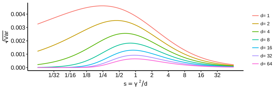
Figure 1: Variance as a function of kernel width $\gamma$ and latent dimensionality $d$. Batch size is fixed to $n=100$.

In the original formulation of the WAE, the MMD penalty enters the objective as the term $\lambda\cdot\mathrm{MMD}^{2}(\mathcal{N}_{d},Q)$, where $\lambda$ is the regularization strength. Obviously, the closed-form formulas for the MMD presented in the previous section can be used instead. In addition, we suggest standardizing the MMD. Since the mean of $\mathrm{MMD}_{u}^{2}$ under the null is zero, and variance under the null is $\mathrm{Var}(\gamma,d,n)$ as given by Eq. (2.3), we define:

$$\mathrm{SMMD}^{2}(Q_{n})\triangleq\frac{\mathrm{MMD}_{u}^{2}(\mathcal{N}_{d},Q_{n})}{\sqrt{\mathrm{Var}(\gamma,d,n)}}.$$

Figure 1 depicts the behavior of the scaling term $\sqrt{\mathrm{Var}(\gamma,d,n)}$ for different values of the kernel width $\gamma$ and the latent dimension $d$, for a fixed batch size $n=100$. We can clearly see that the scaling varies widely not only across dimensions, but also across kernel width choices at a fixed dimension.

While at the theoretical level the suggested scaling can be equivalently seen as a re-definition of the regularization coefficient, yet it has a number of benefits in practice. First, the use of the SMMD is potentially beneficial for model selection.The choice of the best hyperparameters is usually carried out via cross-validation which among others things includes trying out different values of the penalty coefficient $\lambda$, kernel width $\gamma$, and latent dimension $d$. Without the proposed scaling of the MMD term, the values of $\lambda$ are not universal across the choices of $\gamma$ and $d$. For example, if a small list of $\lambda$’s is used when cross-validating, then disparate regions of the optimization space would be considered across the choices of $\gamma$ and $d$, perhaps resulting in a suboptimal model being chosen. Second, our scaled formulation can also be beneficial for the commonly used trick of combining kernels of different widths—using a penalty of the form $\lambda\cdot[\mathrm{MMD}^{2}(\mathcal{N}_{d},Q,\gamma=\gamma_{1})+...+\mathrm{MMD}^{2}(\mathcal{N}_{d},Q,\gamma=\gamma_{k})]$—in order to boost the performance of the MMD and to avoid search over the kernel width. However, when such a combination is performed without the proposed standardization, then MMDs coming from different kernel width choices can be of different orders of magnitude. As a result, one may end up with a single kernel width dominating. In fact, the common choice of including kernels having $s=\gamma^{2}/d\approx 1$ together with the ones that have $s=\gamma^{2}/d\ll 1$ or $\gg 1$ would lead to this issue as can be seen from Figure 1. One can see that this observation is also relevant in cases where $\gamma$ is set adaptively per batch, this time leading to various amounts of penalty being applied to each batch. Third, the most important advantage of using the SMMD is that it is more interpretable and so amenable to quick inspection when one wants to have a sense of how far the current distribution is from the target normal multivariate distribution; this is the focus of the following discussion.

Monitoring WAE Training Progress

It is a standard practice when training a neural network to monitor the progress by inspecting the total loss and its components both for training and validation data. These metrics of interest are computed on a batch level and some type of running averages over the batches are reported. We consider two types of averaging, simple averaging and exponential moving averaging of the SMMD values. For both of these cases we explain how to asses the convergence of code distribution to the standard multivariate normal. As a complementary approach, Appendix B provides thresholds that can be used when monitoring convergence on a single batch level without averaging.

In the case of the simple averaging, the asymptotic distribution under the null is easy to compute. Assume that the validation set contains $m$ batches of size $n$, and the corresponding batches are $Q_{n}^{b}=\{z_{i}^{b}\}_{i=1}^{n},b=1,2,...,m$. The average SMMD value is computed as $B_{m}=\frac{1}{m}\sum_{b=1}^{m}\mathrm{SMMD}^{2}(Q_{n})$, and is the average of independent and identically distributed terms. Under the null, each summand has zero mean and unit variance due to the standardization. Assuming that $m$ is big enough, we can apply the Central Limit Theorem [3], giving that the null distribution of $B_{m}$ is asymptotically normal with mean $0$ and variance $1/m$. Thus, as a rule of thumb, values of $B_{m}$ that do not fall into the three-sigma interval $[-3/\sqrt{m},3/\sqrt{m}]$ should be considered as an indication that the aggregate code distribution has not converged to the target standard multivariate normal distribution. The raw MMD version of this test together with theoretical results can be found in [28], but it is our standardization that makes the test easily applicable by practitioners. [28] called this the B-test, so we will refer to $B_{m}$ as the B-Statistic.

Another popular way of keeping track of progress metrics is exponential moving averaging. The Lyapunov/Lindeberg version of the Central Limit Theorem [3, Chapter 27] can be applied to obtain the corresponding interval. Suppose that the exponential moving average with the momentum of $\alpha$ is used to keep track of a per-batch quantity $S_{b}$. Thus, $E_{b}=\alpha E_{b-1}+(1-\alpha)S_{b}$ is used for $b=1,...,m$. Note that, $E_{m}$ can be written as $E_{m}=\alpha^{m}E_{0}+(1-\alpha)[\alpha^{m-1}S_{1}+\alpha^{m-2}S_{2}+\cdots\alpha S_{m-1}+S_{m}],$ here $S_{0}$ is some initial value, usually $0$, which we will use. Assuming that $S_{b}$ are standardized to have zero mean and unit variance, the application of the CLT to random variables $(1-\alpha)\alpha^{m-k}S_{k}$ gives that $E_{m}$ is normally distributed: $E_{m}\sim\mathcal{N}(0,(1-\alpha^{2m+2})\frac{1-\alpha}{1+\alpha}).$ By dropping $(1-\alpha^{2m+2})$, we can use $(1-\alpha)/(1+\alpha)$ as an upper bound for the variance. This gives the three-sigma interval for the E-Statistic liberally as $[-3\sqrt{(1-\alpha)/(1+\alpha)},3\sqrt{(1-\alpha)/(1+\alpha)}]$. For a common value of $\alpha=0.99$ we get the interval as $[-0.212,0.212]$.

3.2 Code Normalization

In this subsection we propose to apply a variant of batch normalization [14] on top of the code layer before MMD is computed: for each batch, we center and scale the codes so that their distribution has zero mean and unit variance in each dimension; we will refer to this as “code normalization”. Importantly, no scaling or shifting is applied after normalizing (i.e. $\gamma=1$ and $\beta=0$ in the notation of [14]) as the decoder network expects a normally distributed input. Below under separate headings we discuss the benefits of code normalization for the WAE training; we will use the term “MMD penalty” to refer to any kind of penalty based on MMD, including SMMD.

Easier Kernel Width Selection

One advantage of code normalization is that a single setting of the width for the Gaussian RBF kernel, $\gamma$, can be used when computing the MMD penalty. Without code normalization, a fixed choice of $\gamma$ leads to issues. For example, when $\gamma$ is small, and the codes are far away from the origin and from each other, the MMD penalty term has small gradients, which makes learning difficult or even impossible. Indeed, the exponentials become vanishingly small, and since they enter the gradient multiplicatively this makes the gradients small as well. The same issue arises when choosing a large value of $\gamma$ when the codes are not far away from the origin. Thus, one has to use an adaptive choice of $\gamma$ in order to deal with this problem, see e.g. [26]. On the other hand, in the long run, code normalization makes sure that the codes have commensurate distances with $\gamma$ throughout the training process, alleviating the need for an adaptive $\gamma$. This makes possible to decouple the choice of $\gamma$ from the neural network training and to provide practical recommendations as we do in Section 4.

Reduced Training Effort

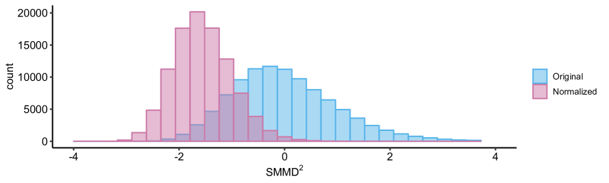
Figure 2: Code normalization shifts the distribution of $\mathrm{SMMD}^{2}$ to lower values. Here, $n=100$, $d=8$, and kernel scale $s=\gamma^{2}/d=1/4$.

Code normalization shifts and scales codes to be in the “right” part of the space, namely where the target standard multivariate normal distribution lives, and we speculate that this reduces the training effort. The intuition comes from inspecting the relationship between the MMD and the characteristic function formulation of the BHEP statistic. This formulation expresses the fact that at some level MMD is performing moment matching, and so by rendering the first two moments (marginal) equal to those of the standard multivariate normal distribution, code normalization focuses the training effort on matching the higher moments.

To illustrate this point, Figure 2 shows the distribution of SMMD values for samples of size $n=100$ taken from $Q=\mathcal{N}_{d}$. The value of SMMD is computed for the original sample and then for the sample to which code normalization was applied. Note that on average the normalized codes have smaller MMD values compared to the original ones. In a sense, normalized samples are more “ideal” from the point of the view of the MMD. This means that even if the neural network has converged to the target normal distribution, the gradient for a batch will not be zero but will have components in the direction of shifting and scaling the codes to reduce the MMD for a given batch. Code normalization directly takes care of this reduction, and allows the training process to spend its effort on improving the reconstruction error. Technically, this is achieved by projecting out the components of the gradient corresponding to shifting and scaling which is automatically achieved by normalization, see [13, Section 3, penultimate paragraph].

This observation reveals an interesting aspect of training with the MMD as compared to training in an adversarial manner [18]. When training in an adversarial manner, the goal is to make the codes in each batch resemble a sample from the standard multivariate normal distribution. At an intuitive level, we expect this would happen with the MMD penalty as well. However, this is not the case—we see that, on average, the MMD penalty considers normalized samples more “ideal” than the actual samples from the target distribution. Luckily, the neural network cannot learn batch-wise operations (e.g. it cannot learn to do batch-wise normalization or whitening by itself) assuming that at inference time the inputs are processed independently of each other. As a result, this phenomenon will not prevent convergence to the target distribution. A rigorous argument follows from unbiasedness, $\mathbb{E}[\mathrm{MMD}_{u}^{2}]=\mathrm{MMD}^{2}\geq 0$ where the expectation is taken over i.i.d. samples and equality holds only at convergence to the target distribution; this makes any overall shift to the left at the inference time impossible.

Remark: When monitoring neural net training the following should be taken into account to avoid wrongly declaring that overfitting has occurred. When code normalization is used, the distribution shift exemplified in Figure 2 will result in a noticeably smaller training loss than the validation loss. This is because code normalization uses the batch statistics during training and population statistics at validation/test time. The difference between these losses can be on the order of several $\lambda$’s; here $\lambda$ is the regularization strength. This effect is akin to substituting an estimator of a parameter (computed from the same data) into a statistic and results in a distributional changes.

Avoiding Outliers

Another benefit of code normalization is that it provides a solution to outlier insensitivity problem of the MMD penalty, described below. Indeed, scaling by the standard deviation (rather than by a robust surrogate) controls the tail behavior of the code distribution. Due to this control, the code distribution ends up having a light tail and no code falls too far away from the origin.

The outlier insensitivity problem is not specific to our closed-form formula or the choice of the kernel (see Section 4 for an empirical verification); this problem is relevant to any kernel $k(x,y)=f(\|x-y\|)$ such that $f(r)\rightarrow 0$ as $r\rightarrow\infty$. Given a sample $Q_{n}=\{z_{i}\}_{i=1}^{n}$ from the standard multi-variate normal distribution, consider a modified sample $Q^{\prime}_{n}=\{z^{\prime}_{i}\}_{i=1}^{n}$, where $z^{\prime}_{i}=z_{i},i=2,...,n$ and $z^{\prime}_{1}$ is far from the origin. Expressing the sum of vanishingly small exponentials via the $O$-notation, we can compute the difference in MMD incurred by this change:

$$\Delta\mathrm{MMD}_{u}^{2} =\mathrm{MMD}_{u}^{2}(Q_{n}^{\prime})-\mathrm{MMD}_{u}^{2}(Q_{n})=$$ (3.1)

$$=\frac{2}{n}\left[\left(\frac{\gamma^{2}}{1+\gamma^{2}}\right)^{d/2}e^{-\frac{\|z_{1}\|^{2}}{2(1+\gamma^{2})}}-\frac{1}{n-1}\sum_{j\neq 1}^{n}e^{-\frac{\|z_{1}-z_{j}\|^{2}}{2\gamma^{2}}}+O\left(e^{-\frac{\|z^{\prime}_{1}\|^{2}}{2(1+\gamma^{2})}}\right)\right]$$

Note that the second term is the sample average approximation of $\mathbb{E}_{x\sim Q=P}[e^{-\|z_{1}-x\|^{2}/(2\gamma^{2})}]$. This expectation can be computed analytically (in fact it is equivalent to the summand in the second term of Eq. (2.2)) and it precisely cancels the first term here in Eq. (3.1), giving $\mathbb{E}[\Delta\mathrm{MMD}_{u}^{2}]\approx 0$. Thus, MMD changes very little despite the presence of the large outlier.

Given the mixed objective and stochasticity inherent in the training process, this issue has an effect on WAE training even before reaching the limits of computer precision. Indeed, in addition to the MMD penalty, the WAE objective contains the reconstruction term. Given the incentive to reconstruct well, the optimizer will realize that it is beneficial to push some of the codes far away from the origin, since the origin is where most of the codes concentrate. If this happens only for a few codes in a batch, the MMD penalty will not be big enough so as to pull these codes back towards the origin. As a result, the training process will result in a distribution $Q$ that has outliers. Our experiments show that the proposed code normalization provides a solution to this issue without a need for using adaptive kernel widths or extra penalties.

4 Experiments

First we discuss our parameterization for the kernel width used in computation of various MMD measures. A rule of thumb choice of the kernel width is $\gamma^{2}=d$, where $d$ is the dimension of the code space (see e.g. [30, 26]). This choice is based on considering the average pair-wise distance between two points drawn from the standard multi-variate normal distribution, and halving it to offset the multiplication by $2$ in the expression for the kernel. We will see that this choice gives rather suboptimal results, yet it provides a good point of reference for defining scale of the kernel as $s=\gamma^{2}/d$. We will experiment with various choices of $s$, where $s>1$ gives wider and $s<1$ gives narrower kernels. The sample size in the experiments is chosen as $n=100$ in agreement with a commonly used batch size while training neural networks.

Validation

We first experimentally verify that our closed-form formula for SMMD results in zero mean and unit variance under the null when $Q=\mathcal{N}_{d}$. To this end, we sample $n=100$ points from the standard $d$-variate normal distribution and compute the value of $\mathrm{SMMD}^{2}$. This process is repeated 10,000 times to obtain the empirical distribution of the values. Figure 1 shows the violin plots of these empirical distributions computed for several values of the kernel scale $s$ and dimensionality $d$. The red segments in this plot are centered at the mean, and they extend between mean $\pm$ standard deviation. We observe from the graph that the means are close to zero and the standard deviations are close to 1 as expected.

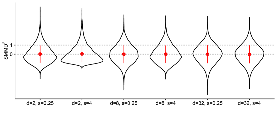
Figure 3: Violin plots verify that $\mathrm{\mathrm{SMMD}^{2}}$ has zero mean and unit variance under the null. Here, batch size is $n=100$ and the kernel width is expressed via the scale $s$ as $\gamma^{2}=s\cdot d$

Discriminative Performance

The goal of the next experiment is to compare our closed-formula estimator of MMD (referred to as “Analytic RBF”) to the standard sampling based estimator using the same Gaussian RBF kernel (“Empirical RBF”). We also compare to the sampling based estimator but with the inverse multi-quadratics (IMQ) kernel defined by $k(x,y)=1/\left(1+\|x-y\|^{2}/(2\gamma^{2})\right)$; we call this “Empirical IMQ”. The IMQ kernel is often claimed to be superior to the RBF kernel due to its slower tail decay.

In our first experiment we would like to determine which one of these three methods is most effective at distinguishing the standard $d$-variate normal distribution from the uniform distribution. Since our goal is to train neural networks rather than perform hypothesis testing, we will not use the test power as a metric of interest; instead we will rely on the effect size defined below. In addition, we are not studying the dependence on the latent dimension, so we do not have to worry about the fair choice of alternatives [22].

Method	Kernel Scale	$d=1$	$d=2$	$d=4$	$d=8$	$d=16$	$d=32$
an RBF	2	$0.49$	$0.14$	$0.05$	$0.02$	$3.7e-04$	$0.11$
	1	$1.18$	$0.7$	$0.29$	$0.09$	$0.04$	$0.03$
	1/2	$1.85$	$1.64$	$0.97$	$0.45$	$0.17$	$0.03$
	1/4	$1.97$	$2.32$	$2.02$	$1.19$	$0.76$	$0.35$
	1/8	$\mathbf{2.28}$	$\mathbf{2.61}$	$\mathbf{2.56}$	$2.01$	$\mathbf{1.5}$	$0.98$
	1/16	$\mathbf{2.21}$	$\mathbf{2.62}$	$\mathbf{2.49}$	$1.88$	$1.39$	$\mathbf{1.17}$
	1/32	$\mathbf{2.22}$	$\mathbf{2.49}$	$2.1$	$1.16$	$0.51$	$0.44$
	HZ	$1.46$	$1.99$	$2.26$	$\mathbf{2.13}$	$\mathbf{1.49}$	$0.39$
emp RBF	2	$0.32$	$0.15$	$0.15$	$9.1e-04$	$0.03$	$0.13$
	1	$0.75$	$0.42$	$0.16$	$0.01$	$0.02$	$0.01$
	1/2	$1.07$	$0.95$	$0.5$	$0.23$	$0.09$	$0.01$
	1/4	$1.36$	$1.34$	$1.1$	$0.66$	$0.3$	$0.14$
	1/8	$1.35$	$\mathbf{1.57}$	$1.3$	$\mathbf{0.99}$	$0.66$	$0.51$
	1/16	$\mathbf{1.4}$	$\mathbf{1.54}$	$\mathbf{1.38}$	$\mathbf{1.02}$	$\mathbf{0.71}$	$\mathbf{0.62}$
	1/32	$\mathbf{1.45}$	$1.36$	$1.1$	$0.57$	$0.26$	$0.15$
	HZ	$1.07$	$1.18$	$1.23$	$\mathbf{0.98}$	$0.64$	$0.25$
emp IMQ	2	$0.51$	$0.29$	$0.08$	$0.06$	$0.01$	$0.03$
	1	$0.74$	$0.48$	$0.27$	$0.12$	$0.06$	$0.03$
	1/2	$1.01$	$0.88$	$0.49$	$0.33$	$0.08$	$0.04$
	1/4	$1.21$	$1.12$	$0.74$	$0.46$	$0.16$	$0.06$
	1/8	$1.23$	$1.36$	$1.1$	$0.45$	$0.2$	$0.1$
	1/16	$\mathbf{1.32}$	$\mathbf{1.41}$	$\mathbf{1.22}$	$0.53$	$0.27$	$0.07$
	1/32	$\mathbf{1.31}$	$\mathbf{1.46}$	$1.19$	$0.61$	$\mathbf{0.32}$	$0.08$
	1/64	$\mathbf{1.33}$	$1.38$	$1.17$	$0.63$	$0.29$	$\mathbf{0.2}$
	1/128	$\mathbf{1.33}$	$\mathbf{1.42}$	$\mathbf{1.26}$	$\mathbf{0.82}$	$\mathbf{0.32}$	$0.08$
	1/256	$\mathbf{1.32}$	$1.26$	$1.19$	$0.63$	$0.28$	$0.13$
	1/512	$1.16$	$1.04$	$1.14$	$0.77$	$0.27$	$0.08$
	1/1024	$1.08$	$1.04$	$1.06$	$0.77$	$\mathbf{0.32}$	$0.11$

Table 1: Discrimination power between $d$-variate standard normal distribution and uniform $U[-\sqrt{3},\sqrt{3}]^{d}$ distribution as measured by $\tau$.

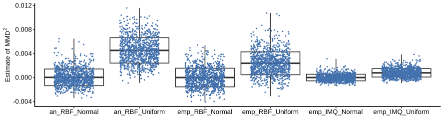
Figure 4: Graphical representation of this discrimination experiment for $d=8$.

Method	Kernel Scale	$d=1$	$d=2$	$d=4$	$d=8$	$d=16$	$d=32$
an RBF	2	$0.17$	$0.12$	$0.11$	$0.11$	$0.1$	$0.1$
	1	$0.35$	$0.33$	$0.43$	$0.5$	$0.39$	$0.31$
	1/2	$0.59$	$0.69$	$1.61$	$1.49$	$1.46$	$1.23$
	1/4	$0.86$	$1.14$	$3.07$	$3.64$	$3.75$	$3.11$
	1/8	$1.1$	$1.42$	$4.6$	$\mathbf{4.95}$	$\mathbf{5.37}$	$\mathbf{4.07}$
	1/16	$1.18$	$1.9$	$\mathbf{4.86}$	$4.71$	$4.24$	$3.21$
	1/32	$\mathbf{1.34}$	$\mathbf{2.1}$	$4.25$	$3.37$	$2.75$	$2.25$
	HZ	$0.52$	$1$	$3.92$	$\mathbf{5.19}$	$4.18$	$2.5$
emp RBF	2	$0.03$	$0.14$	$0.05$	$0.07$	$0.06$	$0.03$
	1	$0.11$	$0.09$	$0.32$	$0.24$	$0.19$	$0.19$
	1/2	$0.24$	$0.46$	$0.88$	$0.81$	$0.72$	$0.59$
	1/4	$0.53$	$0.67$	$1.69$	$1.98$	$2.42$	$2.16$
	1/8	$0.6$	$0.77$	$2.52$	$3.36$	$\mathbf{4.22}$	$\mathbf{3.68}$
	1/16	$0.73$	$0.98$	$\mathbf{2.68}$	$\mathbf{3.74}$	$3.81$	$3.35$
	1/32	$\mathbf{0.78}$	$\mathbf{1.16}$	$2.53$	$3$	$2.69$	$2.11$
	HZ	$0.26$	$0.55$	$2.05$	$\mathbf{3.58}$	$3.86$	$2.41$
emp IMQ	2	$4.7e-03$	$0.19$	$0.25$	$0.16$	$0.12$	$0.16$
	1	$0.16$	$0.26$	$0.49$	$0.33$	$0.43$	$0.34$
	1/2	$0.31$	$0.29$	$0.78$	$0.78$	$0.68$	$0.62$
	1/4	$0.4$	$0.49$	$1.21$	$1.26$	$1.25$	$1.06$
	1/8	$0.51$	$0.73$	$1.78$	$1.85$	$1.73$	$1.47$
	1/16	$0.54$	$0.82$	$2.06$	$2.17$	$2.14$	$1.89$
	1/32	$0.75$	$1.08$	$2.18$	$2.49$	$2.32$	$1.97$
	1/64	$0.92$	$\mathbf{1.18}$	$2.3$	$2.7$	$2.43$	$1.95$
	1/128	$0.89$	$\mathbf{1.24}$	$\mathbf{2.49}$	$2.69$	$\mathbf{2.57}$	$2.11$
	1/256	$0.93$	$\mathbf{1.21}$	$\mathbf{2.46}$	$\mathbf{2.82}$	$\mathbf{2.54}$	$\mathbf{2.22}$
	1/512	$\mathbf{1.11}$	$\mathbf{1.22}$	$2.32$	$\mathbf{2.88}$	$\mathbf{2.58}$	$\mathbf{2.26}$
	1/1024	$\mathbf{1.05}$	$1.15$	$2.23$	$\mathbf{2.77}$	$\mathbf{2.61}$	$\mathbf{2.16}$

Table 2: Discrimination power between the $d$-variate standard normal distribution and a latent $d$-dimensional embedding of MNIST with an unregularized autoencoder.

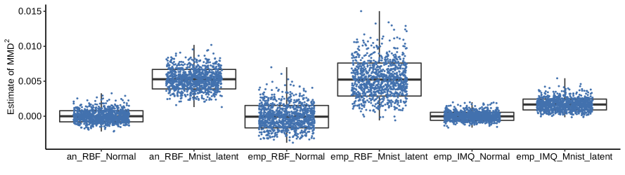
Figure 5: Graphical representation of the discrimination experiment with MNIST latent embedding for $d=8$.

The uniform distribution under consideration is $U[-\sqrt{3},\sqrt{3}]^{d}$. Note that this particular uniform distribution has mean 0 and variance 1 in each dimension just like the normal distribution; distinguishing the two distributions requires going beyond the first two moments. For each of the three methods, for a fixed dimension $d$ and kernel scale $s$, we sample $n=100$ points from the the standard $d$-variate normal distribution and compute the corresponding MMD estimate. Next we sample $n=100$ points from the uniform distribution $U[-\sqrt{3},\sqrt{3}]^{d}$ and compute the corresponding MMD estimate. We repeat this 200 times, and compute the corresponding means $\mathrm{Mean}_{1}$ and $\mathrm{Mean}_{2}$, and the standard deviations $\mathrm{SD}_{1}$ and $\mathrm{SD}_{2}$ corresponding to each of the two sets of 200 MMD values. Now we can measure the discriminativeness of a given method by computing $\tau(\mathrm{method},s,d)=\frac{\mathrm{|Mean}_{1}-\mathrm{Mean}_{2}|}{(\mathrm{SD}_{1}+\mathrm{SD}_{2})/2}.$ Note that this is the effect size of a two sample t-test as measured by Cohen’s d [5]. Larger values of $\tau$ mean better discrimination, which potentially translates to better gradients for neural network training.

The results are presented in Table 1. Note that the experiment was done for different values of the kernel scale; due to the heavier tail, we included more scale choices for the IMQ kernel than for the RBF kernel. For each method and dimensionality choice $d$, the best performing choice of the kernel scale corresponds to the maximum value of $\tau$; these $\tau$ values are shown in boldface (we also highlight the $\tau$ values that are within $5\%$ of the maximum). Figure 4 provides a box-plot display (whiskers span the range of all of the values) for this experiment when $d=8$. In this graph, for each method, the best choice of the kernel scale was used; when the boxes corresponding to normal and uniform distributions overlap, it means that the method has difficulty discriminating the two distributions. In terms of training neural networks, this means that the corresponding MMD penalty may not be able to provide a strong gradient direction for training because the difference is lost within the stochastic noise.

We repeat the same experiment but instead of the uniform distribution we use a distribution obtained from a neural networks. We use the MNIST dataset and train auto-encoders (both encoder and decoder have two hidden layers with 128 neurons each, ReLU activations) with different latent dimensions $d$ with no regularization. The codes corresponding to the test data are extracted and shifted to have zero mean. We observed that with growing $d$ the various latent dimensions were highly correlated (e.g. Pearson correlations as high as $0.4$); thus, to make the task more difficult, we applied PCA-whitening to the latent codes. The resulting discrimination performance is presented in Table 2 and Figure 5.

By examining both of the tables above, we can see that Analytic RBF method outperforms both the Empirical RBF and IMQ methods in terms of discrimination power. Another observation is that the commonly recommended choice of $\gamma^{2}=d$ (which corresponds to the kernel scale $s=1$) is never a good choice; a similar finding for the median heuristic was spelled out in [24]. The kernel width recommended for Henze-Zirkler test gives mixed results, which is somewhat expected—optimality for density estimation does not guarantee optimal discriminative performance. Examining the Analytic RBF results, it seems that kernel scales $s=1/8$ or $s=1/16$ provide a good rule of thumb choices. Finally, in these particular examples we see that despite its having a larger repertoire of kernel scale choices, Empirical IMQ does not perform as well as Empirical RBF. While these results are limited to two datasets, yet they bring into question the commonly recommended choices of the kernel and its width. Of course, our analysis assumes that the alternative distribution has zero mean and unit variance in each dimension. We believe that this is the most relevant setting to WAE learning because during the late stages of WAE training the code distribution starts converging to the normal distribution.

Outliers

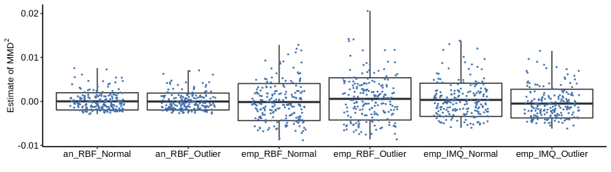
Figure 6: Outlier discrimination experiment carried out for $d=4$. For each method, the most discriminative (i.e. maximum $\tau$) kernel scale is chosen.

Here we experimentally verify the outlier insensitivity of the MMD and demonstrate that the issue is not peculiar to our approach. To this end, we run the discrimination experiment above but this time trying to distinguish a sample from the standard $d$-variate normal distribution from the same but with one of the sample points replaced with a point far away from the origin (namely $z_{1}\rightarrow z^{\prime}_{1}=100\cdot\vec{1}$). Figure 6 shows that all of the three methods fail to distinguish these two distributions in practice.

Code Norm (60 epochs)
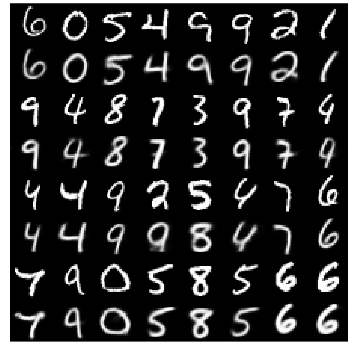
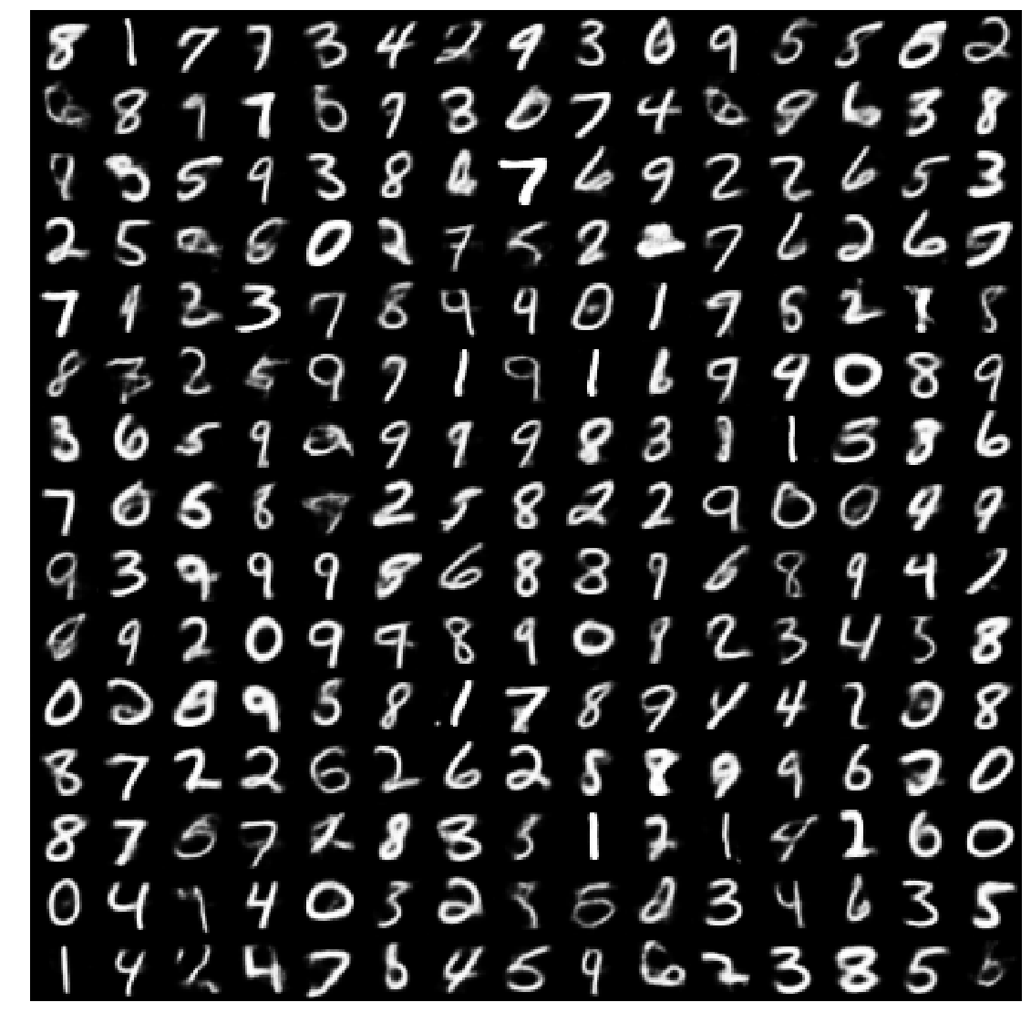
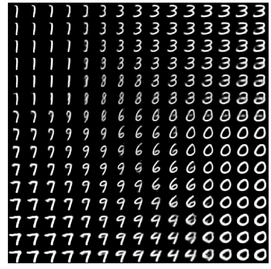
AdaptiveBN (80 epochs)
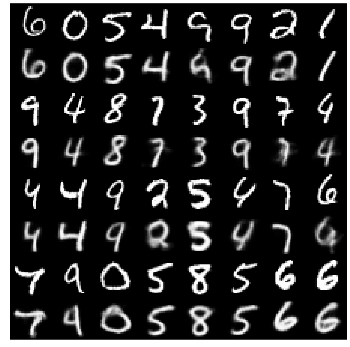
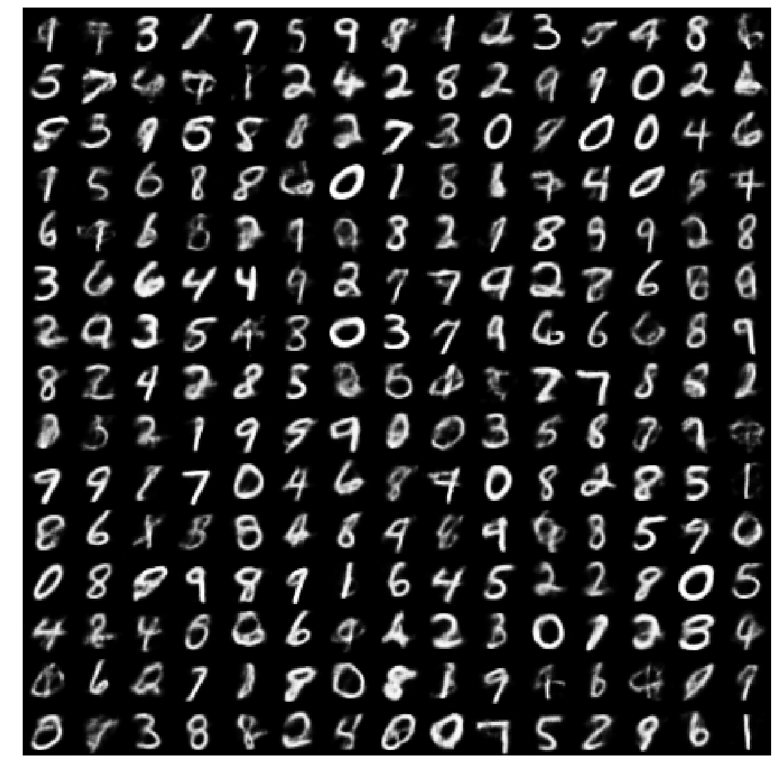
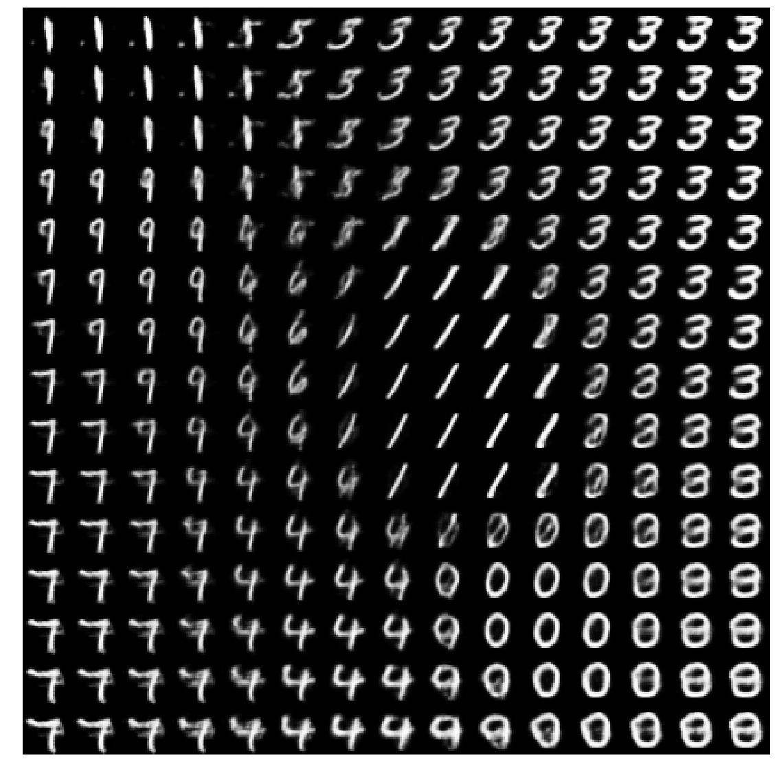
AdaptivePlain (80 epochs)
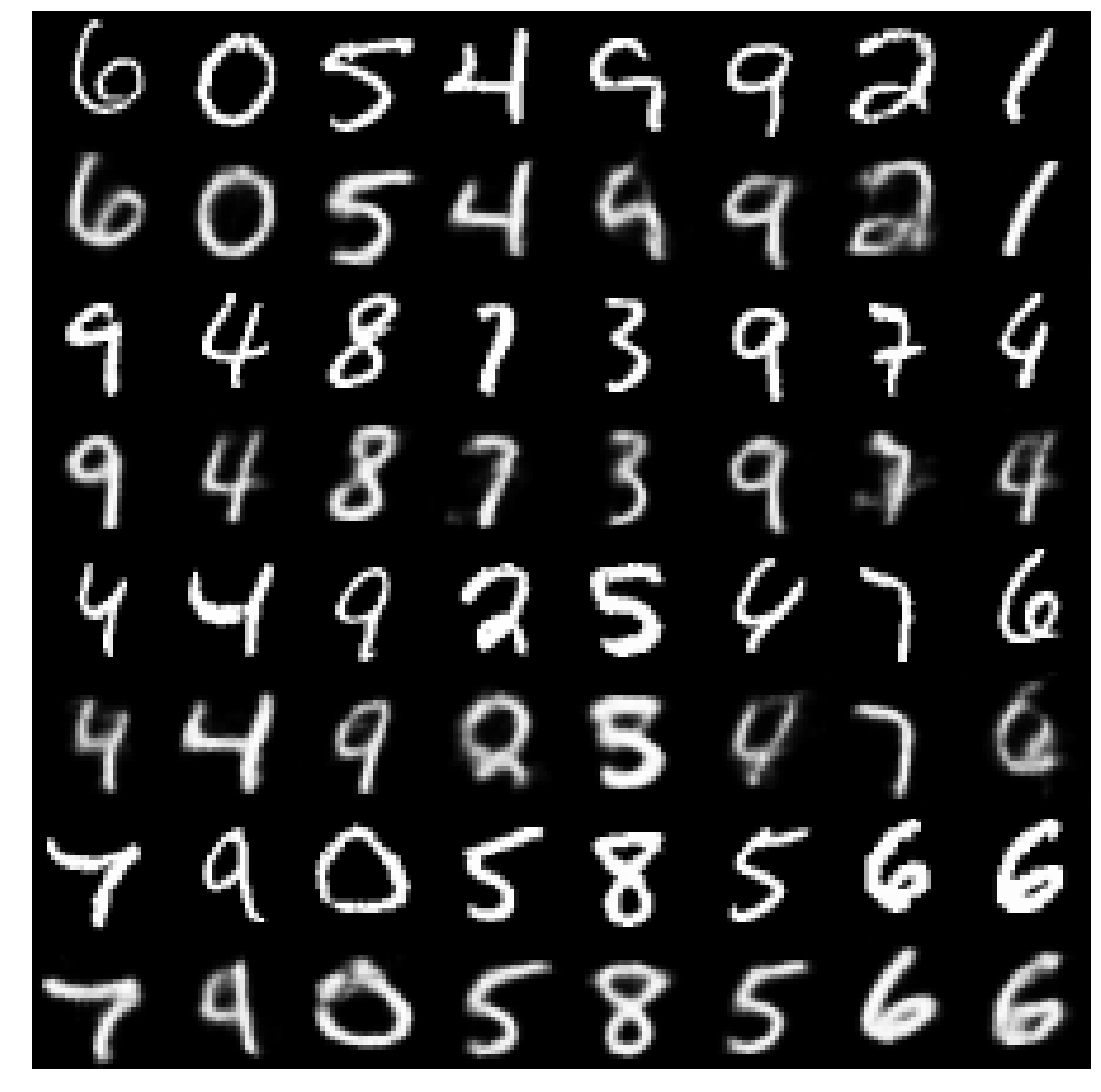
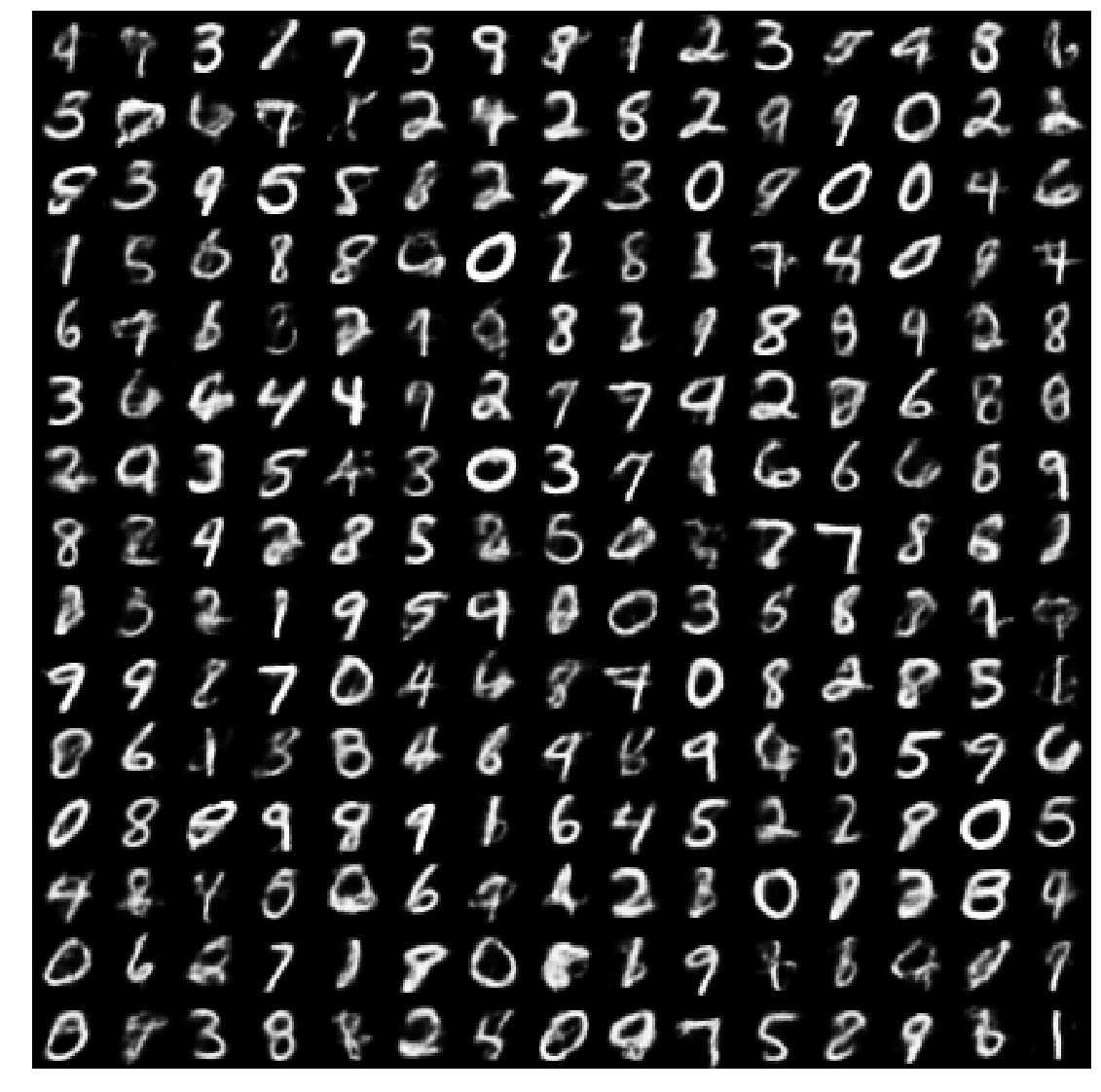
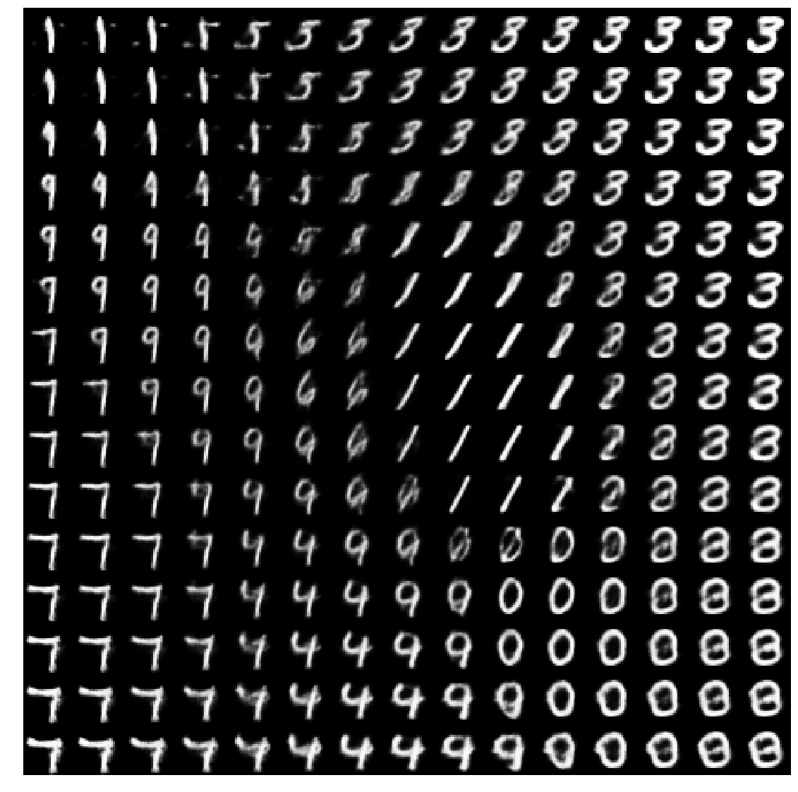
	a) Test reconstruction	b) Random samples	c) Slice through code space

Figure 7: Qualitative results for WAE trained on MNIST. In (a) odd rows are the real images.

WAE results

Here we present the results of training WAEs on MNIST dataset. The architecture for the neural net is borrowed from RStudio’s “Keras Variational Auto-encoder with Deconvolutions” example. This network has about 3.5M trainable parameters, almost an order of magnitude less than the the 22M parameter network used by Tolstikhin et al. [26]. We consider three versions:

• CodeNorm—code normalization is used, the kernel width is kept fixed.

• Adaptive—no code normalization is used, kernel width is chosen adaptively. This has two versions:

  • AdaptiveBN—since code normalization can have other benefits (e.g. improved optimization [23]), we add batch normalization as the initial layer of the decoder;

  • AdaptivePlain—no batch normalization layer added at all.

The CodeNorm version was trained for 60 epochs, but to allow the Adaptive versions to reach a favorable configuration in the code space we trained them for an extra 20 epochs at the initial learning rate. The latent dimension is set to $d=8$ and all versions use the closed-form SMMD penalty for fairness; further details are provided in the Appendix D.

Figure 7 (a)-(b) shows the reconstruction of test images and random samples generated from Gaussian noise fed to the decoder. We also take a planar slice through the origin in the code space and feed the codes at the regular grid along this plane into the decoder. Figure 7 (c) depicts the resulting digit images, giving a taste of the manifold structure captured by the models. Qualitatively, both of the Adaptive results are lower quality than CodeNorm despite the former being trained for more epochs. Quantitative results are presented in Table 3. CodeNorm achieves the best test reconstruction error. We speculate that the reason for this is that the gradient components of the MMD penalty pointing in the direction of “ideal” samples (see Section 3.2) add oscillations that hinder reduction in the reconstruction loss of the Adaptive models.

Next, we follow the suggestion of [25] to compute Mardia’s multivariate skewness and normalized kurtosis statistics of the latent code distribution of test data; we used the formulas provided in [25] and obtained the values as shown in the table. We see that for both measures, the CodeNorm version is better. Skewness is a measure of symmetry, so its small magnitude indicates that the code distribution is symmetrically distributed around the origin. Since kurtosis is a measure of outlier presence [27], its small value indicates that there are no outliers present in the code distribution. We verified experimentally (not presented here) that code normalization is responsible for keeping kurtosis under control. Indeed, removing the code normalization layer from a trained network, modifying the latent layer incoming weights so that the codes have zero mean and unit variance, and continuing to train afterwards leads to increased kurtosis as predicted in Section 3.2.

Finally, we analyze the results using the B-statistic discussed in Section 3. We computed the B-statistic using $m=50$ batches of size $n=100$ from the test partition of MNIST. The corresponding three sigma interval is $[-3/\sqrt{50},3/\sqrt{50}]=[-0.424,0.424]$. Both CodeNorm and AdaptiveBN look good in terms of this statistic, CodeNorm falling inside the interval; on the other hand AdaptivePlain is somewhat farther away, indicating that its code distribution more noticeably deviates from the target distribution.

WAE Version	Test MSE	Normalized Kurtosis	Skewness	B-Statistic
CodeNorm	0.0156	-0.90	0.56	0.355
AdaptiveBN	0.0244	6.85	2.80	0.449
AdaptivePlain	0.0242	3.81	2.35	0.519

Table 3: Quantitative comparison of different WAE versions.

5 Conclusion

We have introduced closed-form formulas for MMD, pointed out a relationship with the BHEP statistic, and provided suggestions for WAE training and monitoring. Our experiments confirm that the analytic formulation improves over the stochastic approximation of the MMD, and demonstrate that code normalization provides significant benefits when training WAEs. An interesting avenue for future work is to investigate using the unbiased MMD estimator for hypothesis testing instead of the BHEP statistic. New analytic results would be needed to compute the variance of this statistic for the composite null hypothesis of multivariate normality and perhaps the asymptotic estimates from the MMD literature can be used to determine testing thresholds.

Appendix A Random Encoders

A.1 MMD Formula

In this section we consider Gaussian random encoders, where instead of one code per input data point, we obtain a distribution of codes given as $z_{i}\sim N(\mu_{i},\Sigma_{i}),i=1,2,...,n$. Here $n$ is the batch size, $\Sigma_{i}$ is a diagonal covariance matrix, $\Sigma_{i}=\mathrm{diag}(\sigma_{i1}^{2},\sigma_{i2}^{2},...,\sigma_{id}^{2})$. Both mean vectors $\mu_{i}\in\mathbb{R}^{d}$ and variance vectors $\sigma_{i}\in\mathbb{R_{+}}^{d}$ are computed by applying neural nets to the input data. Our goals is once again to obtain an estimator for $\mathrm{MMD^{2}}(\mathcal{N}_{d}(\vec{0},I),Q)$.

Note that the implied distribution of $Q$ for the current batch is an equally weighted mixture of Gaussians $Q_{\mathrm{batch}}$ with the distribution given by:

$$q_{\mathrm{batch}}(z)\sim\frac{1}{n}\sum_{i=1}^{n}\prod_{k=1}^{d}\frac{e^{-(z_{k}-\mu_{ik})^{2}/(2\sigma_{ik}^{2})}}{\sqrt{2\pi\sigma_{ik}^{2}}},$$

where we $z_{k}$ is the $k$-th component of the vector $z\in\mathbb{R}^{d}$. We will replace sampling from $Q$ in the formula for MMD, Eq. (2.1), by sampling from $Q_{\mathrm{batch}}$, and compute the second and third terms in a closed form. Note that the first term depends only on $P$ and will be the same as before; the computation of the remaining terms is demonstrated in Section C.2, and yields the following unbiased estimator:

$$\mathrm{MMD}_{u}^{2}(\mathcal{N}_{d}(\vec{0},I),Q_{\mathrm{batch}})= \left(\frac{\gamma^{2}}{2+\gamma^{2}}\right)^{d/2}-\frac{2}{n}\sum_{i=1}^{n}\prod_{k=1}^{d}\left(\frac{\gamma^{2}}{1+\gamma^{2}+\sigma_{ik}^{2}}\right)^{1/2}e^{-\frac{\mu_{ik}{}^{2}}{2(1+\gamma^{2}+\sigma_{ik}^{2})}}+$$

$$+ \frac{1}{n^{2}}\sum_{i=1}^{n}\sum_{j=1}^{n}\prod_{k=1}^{d}\left(\frac{\gamma^{2}}{\gamma^{2}+\sigma_{ik}^{2}+\sigma_{jk}^{2}}\right)^{1/2}e^{-\frac{(\mu_{ik}-\mu_{jk}){}^{2}}{2(\gamma^{2}+\sigma_{ik}^{2}+\sigma_{jk}^{2})}}.$$

When the noise is isotropic, namely $\Sigma_{i}=\mathrm{diag}(\sigma_{i}^{2},\sigma_{i}^{2},...,\sigma_{i}^{2})$ with $\sigma_{i}\in\mathbb{R_{+}}$(note that $\sigma_{i}$ was a vector in the general case above, but here it is a single number), we can rewrite this formula in a simpler form:

$$\mathrm{MMD}_{u}^{2}(\mathcal{N}_{d}(\vec{0},I),Q)= \left(\frac{\gamma^{2}}{2+\gamma^{2}}\right)^{d/2}-\frac{2}{n}\sum_{i=1}^{n}\left(\frac{\gamma^{2}}{1+\gamma^{2}+\sigma_{i}^{2}}\right)^{d/2}e^{-\frac{\|\mu_{i}\|{}^{2}}{2(1+\gamma^{2}+\sigma_{i}^{2})}}+$$

$$+ \frac{1}{n^{2}}\sum_{i=1}^{n}\sum_{j=1}^{n}\left(\frac{\gamma^{2}}{\gamma^{2}+\sigma_{i}^{2}+\sigma_{j}^{2}}\right)^{d/2}e^{-\frac{\|\mu_{i}-\mu_{j}\|{}^{2}}{2(\gamma^{2}+\sigma_{i}^{2}+\sigma_{j}^{2})}}.$$

Note that setting the variances $\sigma_{i}^{2}=0$ gives rise to the deterministic encoders where $z_{i}=\mu_{i}$, and the resulting estimator is the same as $\mathrm{MMD}_{b}^{2}$ and not $\mathrm{MMD}_{u}^{2}$. The difference is that the last term in the unbiased deterministic estimator includes an average over distinct pairs $(i,j),i\neq j$, whereas for the unbiased random estimator the average runs over all pairs $(i,j)$. The latter is appropriate here because when $\sigma_{i}^{2}\neq 0$, in Eq. (2.1) one can sample $y,y^{\prime}\sim Q_{\mathrm{batch}}$ independently from the same component of the Gaussian mixture. Doing so in the deterministic case would have resulted in a biased estimate: essentially instead of the U-statistic we would have gotten the upwards biased V-statistic.

A.2 Code Normalization

Random encoders require a separate treatment of the mean and variance network outputs. Namely, using the above notation, code normalization is given in coordinate-wise manner by

$$\mu_{\cdot k}\rightarrow(\mu_{\cdot k}-\mathrm{Mean}_{k}(Q_{\mathrm{batch}}))/\mathrm{SD}_{k}(Q_{\mathrm{batch}}),\>\mathrm{and\quad}\sigma_{\cdot k}\rightarrow\sigma_{\cdot k}/\mathrm{SD}_{k}(Q_{\mathrm{batch}}),$$

where subscript $k$ is used to refer to the $k$-th coordinate, $k=1,2,...,d$, and $\mathrm{SD}_{k}(Q_{\mathrm{batch}})=\sqrt{\mathrm{Var}_{k}(Q_{\mathrm{batch}})}$. Since $Q_{\mathrm{batch}}$ is a mixture of Gaussians, closed form expressions for mean and variance are available:

$$\mathrm{Mean}_{k}(Q_{\mathrm{batch}})=\frac{1}{n}\sum_{i=1}^{n}\mu_{ik},\>\mathrm{and}\qquad\mathrm{Var}_{k}(Q_{\mathrm{batch}})=\frac{1}{n}\sum_{i=1}^{n}(\mu_{ik}^{2}+\sigma_{ik}^{2})-\left(\frac{1}{n}\sum_{i=1}^{n}\mu_{ik}\right)^{2}.$$

Appendix B Hypothesis Tests for Multivariate Normality

In this section we discuss hypothesis testing using $\mathrm{SMMD}^{2}$ and provide thresholds that can be useful when monitoring progress of WAE code distribution convergence on a single batch level. Note that the discussion in the main text was limited to multi-batch testing setup which had a simple null distribution due to the CLT. Our initial discussion is set in a broader manner so as to encompass general testing for multivariate normality.

We quickly review the hypothesis testing setting following [11] with some notational changes. Let $X_{1},X_{2},...,X_{n}\in\mathbb{R}^{d}$ be i.i.d. random vectors from some underlying distribution. The problem is to test the hypothesis that the underlying distribution is a non-degenerate $d$-variate normal distribution: $X_{i}\sim\mathcal{N}_{d}(\vec{\mu},\Sigma)$, for some mean vector $\vec{\mu}$ and non-degenerate covariance matrix $\Sigma$. Note that the population mean vector and covariance matrix are not known.

The test of multivariate normality proceeds as follows. Let $\bar{X}=n^{-1}\sum_{i}X_{i}$ be the sample mean, and $S=(n-1)^{-1}\sum_{i}(X_{i}-\bar{X})(X_{i}-\bar{X})^{T}$ be the sample covariance matrix. Assuming non-degeneracy, define the centered and whitened vectors

$$Z_{i}=S^{-1/2}(X_{i}-\bar{X}).$$

Now, the task of testing multivariate normality of $\{X_{i}\}_{i=1}^{n}$ reduces to the simpler problem of testing whether the underlying distribution of $\{Z_{i}\}_{i=1}^{n}$ is $\mathcal{N}_{d}(\vec{0},I)$.

While Henze-Zirkler test [11] carries out this last step by using the BHEP statistic, it can also be achieved by using the $\mathrm{SMMD}^{2}$. One computes the $\mathrm{SMMD}^{2}$ statistic for the sample $\{Z_{i}\}_{i=1}^{n}$ and checks whether it is above the test threshold, and if so, the null hypothesis gets rejected. The most straightforward way to compute the threshold is to run a Monte Carlo simulation: sample $\{Z_{i}\}_{i=1}^{n}$ from the null distribution $\mathcal{N}_{d}(\vec{0},I)$, and compute the corresponding $\mathrm{SMMD}^{2}$ value; repeat this many times to obtain the empirical sampling distribution of the statistic and use the $100\cdot(1-\alpha)$-th percentile as the threshold for the $\alpha$-level test.

However, this approach is problematic due to the treatment of the nuisance parameters $\vec{\mu}$ and $\Sigma$: the same sample is used both for estimating mean and covariance, and then for testing (this is somewhat like training and testing on the same data). The most apparent consequence is that one introduces dependencies within $\{Z_{i}\}_{i=1}^{n}$, namely, $n^{-1}\sum_{i}Z_{i}=\vec{0}$ and $(n-1)^{-1}\sum_{i}Z_{i}Z_{i}^{T}=I_{d}$, rendering it no longer an i.i.d sample. Thus, when using the Monte Carlo approach with $\{Z_{i}\}_{i=1}^{n}$ sampled directly from $\mathcal{N}_{d}(\vec{0},I)$ we would end up with a wrong null distribution and, so, with the wrong thresholds. Henze-Zirkler test [11] uses appropriate corrections to account for the nuisance parameters when computing the moments under the null. These moments are then used to obtain a log-normal approximation to the null distribution. A similar path can be potentially taken with the $\mathrm{SMMD}^{2}$ statistic, but for simplicity we will explain how to correct the issue with Monte Carlo sampling.

To fix the problem, the computation of the null distribution should proceed from samples that satisfy the dependency relationships mentioned above. Fortunately, constructing such samples is easy: we sample $\{Z_{i}^{\mathrm{orig}}\}_{i=1}^{n}$ from $\mathcal{N}_{d}(\vec{0},I)$, then apply centering by the mean and whitening by the sample covariance matrix. The resulting sample $\{Z_{i}\}_{i=1}^{n}$ satisfies the relationships $n^{-1}\sum_{i}Z_{i}=\vec{0}$ and $(n-1)^{-1}\sum_{i}Z_{i}Z_{i}^{T}=I_{d}$. This centered and whitened sample is used to compute the $\mathrm{SMMD}^{2}$ values and to obtain the thresholds. To prove the correctness of this procedure one has to show that there is a measure preserving and test statistic preserving one-to-one mapping between these samples originating from $\mathcal{N}_{d}(\vec{0},I)$ and samples if they were to originate from $\mathcal{N}_{d}(\vec{\mu},\Sigma)$ with the true $\vec{\mu}$ and $\Sigma$. Using the non-degeneracy of $\Sigma$, with some linear algebra one can show that indeed there is such a mapping given by an orthogonal linear transformation, see Section C.3. The matrix of this transformation depends on $\Sigma$ only, making it measure preserving. Since $\mathrm{SMMD}^{2}$ is rotation-invariant, the resulting sampling distributions coincide.

Before proceeding, we would like to mention a modification of the above test where the goal is to test whether the sample comes from a normal distribution with a diagonal covariance. This is a test that both checks each dimension for normality and establishes the independence between the dimensions. When conducting the test only the diagonal of the sample covariance matrix is computed and used for transforming $\{X_{i}\}_{i=1}^{n}$ to $\{Z_{i}\}_{i=1}^{n}$. The corresponding Monte Carlo procedure takes $\{Z_{i}^{\mathrm{orig}}\}_{i=1}^{n}$ from $\mathcal{N}_{d}(\vec{0},I)$, and applies centering by the mean and scaling each dimension by its standard deviation (just like code normalization).

Table 4 displays the thresholds corresponding to the $0.05$ level test, for sample size of $n=100$ for varying dimensions and kernel scales (we have included dimensions $16$ and $32$ to give an idea about the overall trend; one expects the test to lose power with an increasing dimensionality [22]). The column “Sample Type” indicates what processing was applied to the original sample $\{Z_{i}^{\mathrm{orig}}\}_{i=1}^{n}$ from $\mathcal{N}_{d}(\vec{0},I)$, if any. The “Original” thresholds can be used for testing the following simple hypothesis: given a sample $\{X_{i}\}_{i=1}^{n}$ we would like to test whether the underlying distribution is $\mathcal{N}_{d}(\vec{0},I)$. The “Centered+Scaled” and “Centered+Whitened” rows give the correct thresholds for composite nulls, i.e. testing whether $X_{i}\sim\mathcal{N}_{d}(\vec{\mu},\Sigma)$, for unknown $\vec{\mu}$ and $\Sigma$. “Centered+Scaled” corresponds to the case where $\Sigma$ is assumed to be diagonal, and “Centered+Whitened” correspond to the case of a general non-degenerate $\Sigma$. As expected, dependencies within the sample shift the null distribution of $\mathrm{SMMD}^{2}$ to the left considerably; also see Figure 2 in the main text for side by side histograms of “Centered+Scaled” versus “Original” null distributions. Therefore, using the original thresholds for composite hypotheses would have resulted in tests that are rather liberal.

Dimension	Sample Type	$s=1$	1/2	1/4	1/8	1/16	HZ
$d=1$	Original	1.97	1.97	1.95	1.92	1.91	1.98
	Centered+Scaled/Whitened	-0.13	0.32	0.75	1.05	1.24	0.22
$d=2$	Original	1.93	1.94	1.90	1.85	1.83	1.90
	Centered+Scaled	-0.57	-0.12	0.39	0.86	1.16	0.23
	Centered+Whitened	-0.79	-0.33	0.22	0.72	1.06	0.03
$d=4$	Original	1.90	1.87	1.83	1.79	1.76	1.83
	Centered+Scaled	-1.09	-0.66	-0.02	0.63	1.12	0.30
	Centered+Whitened	-1.60	-1.25	-0.56	0.24	0.85	-0.16
$d=8$	Original	1.85	1.83	1.80	1.77	1.74	1.75
	Centered+Scaled	-1.76	-1.36	-0.59	0.34	1.11	0.55
	Centered+Whitened	-2.63	-2.57	-1.88	-0.60	0.58	-0.30
$d=16$	Original	1.81	1.80	1.77	1.74	1.78	1.78
	Centered+Scaled	-2.65	-2.30	-1.47	-0.15	1.08	1.05
	Centered+Whitened	-4.00	-4.47	-4.17	-2.31	0.00	-0.03
$d=32$	Original	1.77	1.77	1.74	1.71	1.76	1.30
	Centered+Scaled	-3.87	-3.59	-2.78	-1.13	0.75	1.02
	Centered+Whitened	-5.86	-7.12	-7.91	-5.72	-1.24	0.06

Table 4: Empirical thresholds for hypothesis tests with size $\alpha=0.05$. See text for the details of when each kind of threshold should be used. Here, $n=100$, kernel scale $s=\gamma^{2}/d$. HZ is the $\gamma$ suggested by Henze and Zirkler [11], see the main article for the formula.

Monitoring WAE Training Progress

We can consider two ways of monitoring progress: at a single batch and multi-batch levels; the multi-batch version is explained in Section 3.1 of the main text under the heading “Monitoring WAE Training Progress”. When inspecting the value of $\mathrm{SMMD}^{2}$ for a single batch, one can use the above thresholds for hypothesis testing as a guideline. Assuming that this batch is from validation or test set, we can use the above thresholds listed in the “Original” rows of Table 4. By looking at these values, we suggest using $2.0$ as an easy to remember liberal threshold. This applies to code normalized batches as long as the normalization is done using population statistics. However, when the batch is normalized using its own statistics, then the appropriate thresholds are given by the “Centered+Scaled” rows. We should stress again that even upon convergence to the target distribution, one should still expect oscillations of the $\mathrm{SMMD}^{2}$ values: it is not the case that samples from the target distribution all have $\mathrm{SMMD}^{2}$ equal to zero, instead they follow the appropriate null distribution.

Of course, the single-batch approach above that treats the whole validation/test set as one batch would result in a more powerful test. However, the multi-batch B-statistic or E-statistic tests are simple to state and are computationally inexpensive as they avoid constructing the large pair-wise distance matrices for the overall test. Moreover, neural network packages such as Keras provide these types of averages automatically if one adds the corresponding quantity as a validation metric. At a theoretical level, one should keep in mind that given enough power we will always reject the null: with real-life data one rarely expects the neural net to exactly reproduce the normal distribution. Rejecting the null at high power does not mean that the distributions are easily distinguishable: the practical difference can be so small that a classifier trained to distinguish the two distributions (think of an adversary from an adversarial WAE) would perform at a nearly chance level. Based on these considerations, using the B-Statistic with $m=30-50$ should be a reasonable choice, see the discussion in [9, Appendix 1] albeit in a different context; for power calculations for the MMD based tests one can refer to [24].

Appendix C Derivations and Proofs

C.1 Deterministic Encoders

We start with the expression

$$\mathrm{MMD}_{u}^{2}(\mathcal{N}_{d},Q_{n})=\mathbb{E}_{x,x^{\prime}\sim\mathcal{N}_{d}}[k(x,x^{\prime})]-\frac{2}{n}\sum_{i=1}^{n}\mathbb{E}_{x\sim\mathcal{N}_{d}}[k(x,z_{i})]+\frac{1}{n(n-1)}\sum_{i=1}^{n}\sum_{j\neq i}^{n}k(z_{i},z_{j}).$$ (C.1)

and show that the first two expectations can be computed in closed form. Let us start with the second term, and rewrite each summand as an integral:

$$\mathbb{E}_{x\sim P}[k(x,z)]= \int_{\mathbb{R}^{d}}e^{-\|x-z\|^{2}/(2\gamma^{2})}(2\pi)^{-d/2}e^{-\|x\|^{2}/2}dx$$

$$= (2\pi\gamma^{2})^{d/2}\int_{\mathbb{R}^{d}}(2\pi\gamma^{2})^{-d/2}e^{-\|x-z\|^{2}/(2\gamma^{2})}(2\pi)^{-d/2}e^{-\|x\|^{2}/2}dx.$$ (C.2)

Since $\|x-z\|^{2}=\|z-x\|^{2}$, the integral in this expression can be recognized as the probability density function of the sum $Z=U+V$ where $U\sim N(\vec{0},\gamma^{2}I)$ and $V\sim N(\vec{0},I)$. Being a sum of two normal distributions, adding means and variances we get, $Z\sim N(\vec{0},(1+\gamma^{2})I)$, and the above expression computes to

$$\mathbb{E}_{x\sim P}[k(x,z)]=(2\pi\gamma^{2})^{d/2}(2\pi(1+\gamma^{2}))^{-d/2}e^{-\frac{\|z\|^{2}}{2(1+\gamma^{2})}}=\left(\frac{\gamma^{2}}{1+\gamma^{2}}\right)^{d/2}e^{-\frac{\|z\|^{2}}{2(1+\gamma^{2})}}.$$ (C.3)

Next, we compute the first term in Eq. (C.1) by rewriting it as an integral:

$$\mathbb{E}_{x,x^{\prime}\sim P}[k(x,x^{\prime})]=$$

$$= \int_{\mathbb{R}^{d}}\int_{\mathbb{R}^{d}}e^{-\|x-x^{\prime}\|^{2}/(2\gamma^{2})}(2\pi)^{-d/2}e^{-\|x\|^{2}/2}(2\pi)^{-d/2}e^{-\|x^{\prime}\|^{2}/2}dxdx^{\prime}.$$ (C.4)

In this expression, let us replace $e^{-\|x^{\prime}\|^{2}/2}$ by $e^{-\|x^{\prime}-w\|^{2}/2}$, and remember that we would get the sought value by setting $w=\vec{0}$. Rewriting this as

$$(2\pi\gamma^{2})^{d/2}\int_{\mathbb{R}^{d}}\left(\int_{\mathbb{R}^{d}}(2\pi\gamma^{2})^{-d/2}e^{-\|x-x^{\prime}\|^{2}/(2\gamma^{2})}(2\pi)^{-d/2}e^{-\|x\|^{2}/2}dx\right)(2\pi)^{-d/2}e^{-\|x^{\prime}-w\|^{2}/2}dx^{\prime},$$ (C.5)

With this replacement, we can recognize the inner integral as the density function of the sum of two multivariate normal variables. Interpreting the outer integral similarly, we can see that the entire double integral captures the probability density function of the sum $W=A+B+C$, where $A\sim N(\vec{0},\gamma^{2}I)$, $B\sim N(\vec{0},I)$ and $C\sim N(\vec{0},I)$. Being a sum of three normal distributions, adding means and variances we get $W\sim N(\vec{0},(2+\gamma^{2})I)$, immediately giving the expression for this integral as

$$(2\pi(2+\gamma^{2}))^{-d/2}e^{-\frac{\|w\|^{2}}{2(2+\gamma^{2})}}$$

Including the multiplier in front of the integral, and setting $w=\vec{0}$, we obtain:

$$\mathbb{E}_{x,x^{\prime}\sim P}[k(x,x^{\prime})]=\left(\frac{\gamma^{2}}{2+\gamma^{2}}\right)^{d/2}.$$

Putting everything together we obtain the closed-form formula for $\mathrm{MMD}_{u}^{2}(\mathcal{N}_{d},Q_{n})$.

Variance

Since its computation involves taking a random sample from $Q$, we see that $\mathrm{MMD}_{u}^{2}$ is a random variable. Thus, even when $Q=P=\mathcal{N}_{d}$, the estimator $\mathrm{MMD}_{u}^{2}(\mathcal{N}_{d},Q_{n})$ will not be identically zero. It is important to understand the behavior of this random variable; using the hypothesis testing terminology, we refer to this as the distribution of $\mathrm{MMD}_{u}^{2}$ under the null—the null hypothesis being $Q=P=\mathcal{N}_{d}$. By unbiasedness, we have that the null mean is zero:

$$\mathbb{E}[\mathrm{MMD}_{u}^{2}(\mathcal{N}_{d},Q_{n}))]=\mathrm{MMD}^{2}(\mathcal{N}_{d},\mathcal{N}_{d})=0,$$

where the expectation is over various realizations of the sample $Q_{n}=\{z_{i}\}_{i=1}^{n}$ from $Q=\mathcal{N}_{d}$. This immediately means that in contrast to $\mathrm{MMD}^{2}$, the estimator $\mathrm{MMD}_{u}^{2}$ can take negative values.

Next, we would like to obtain the variance $\mathrm{MMD}_{u}^{2}$ under the null. First, we rewrite $\mathrm{MMD}_{u}^{2}$ by defining,

$$h(z,z^{\prime})=\left(\frac{\gamma^{2}}{2+\gamma^{2}}\right)^{d/2}-\left(\frac{\gamma^{2}}{1+\gamma^{2}}\right)^{d/2}e^{-\frac{\|z\|^{2}}{2(1+\gamma^{2})}}-\left(\frac{\gamma^{2}}{1+\gamma^{2}}\right)^{d/2}e^{-\frac{\|z^{\prime}\|^{2}}{2(1+\gamma^{2})}}+e^{-\frac{\|z-z^{\prime}\|^{2}}{2\gamma^{2}}},$$

and noting that

$$\mathrm{MMD}_{u}^{2}(\mathcal{N}_{d},Q_{n})=\frac{1}{n(n-1)}\sum_{i=1}^{n}\sum_{j\neq i}^{n}h(z_{i},z_{j}).$$

Now according to [10, Appendix B.3 ] we have

$$\mathbb{E}\left[\left(\mathrm{MMD}_{u}^{2}(\mathcal{N}_{d},Q_{n})\right)^{2}\right]=\frac{2}{n(n-1)}E_{z,z^{\prime}\sim\mathcal{N}_{d}}[h^{2}(z,z^{\prime})].$$

This expression can be computed in a closed form using manipulations similar to those used for computing $\mathrm{MMD}_{u}^{2}$. Since the mean of $\mathrm{MMD}_{u}^{2}$ under the null is $0$, the null variance is equal to the second moment, and we obtain the formula,

$$\mathrm{Var}(\gamma,d,n)\triangleq \mathbb{E}\left[\left(\mathrm{MMD}_{u}^{2}(\mathcal{N}_{d},Q_{n})\right)^{2}\right]=$$

$$= \frac{2}{n(n-1)}\left[\left(\frac{\gamma^{2}}{2+\gamma^{2}}\right)^{d}+\left(\frac{\gamma^{2}}{4+\gamma^{2}}\right)^{d/2}-2\left(\frac{\gamma^{4}}{(1+\gamma^{2})(3+\gamma^{2})}\right)^{d/2}\right]$$ (C.6)

C.2 Random Encoders

Let us start by computing the second term in Eq. (2.1), namely

$$\mathbb{E}_{x\sim P,y\sim Q_{\mathrm{batch}}}[k(x,y)] =\int_{\mathbb{R}^{d}}\int_{\mathbb{R}^{d}}\left(\frac{1}{n}\sum_{i=1}^{n}\prod_{k=1}^{d}\frac{e^{-(y_{k}-\mu_{ik})^{2}/(2\sigma_{ik}^{2})}}{\sqrt{2\pi\sigma_{ik}^{2}}}\right)\cdot e^{-\frac{\|x-y\|^{2}}{2\gamma^{2}}}(2\pi)^{-d/2}e^{-\frac{\|x\|^{2}}{2}}dxdy$$

$$= \int_{\mathbb{R}^{d}}\int_{\mathbb{R}^{d}}\left(\frac{1}{n}\sum_{i=1}^{n}\prod_{k=1}^{d}\frac{e^{-(y_{k}-\mu_{ik})^{2}/(2\sigma_{ik}^{2})}}{\sqrt{2\pi\sigma_{ik}^{2}}}\right)\cdot\prod_{k=1}^{d}\frac{e^{-\frac{(x_{k}-y_{k}){}^{2}}{2\gamma^{2}}}e^{-\frac{x_{k}^{2}}{2}}}{\sqrt{2\pi}}dxdy$$

$$= \frac{1}{n}\sum_{i=1}^{n}\int_{\mathbb{R}^{d}}\int_{\mathbb{R}^{d}}\prod_{k=1}^{d}\frac{e^{-(y_{k}-\mu_{ik})^{2}/(2\sigma_{ik}^{2})}e^{-\frac{(x_{k}-y_{k}){}^{2}}{2\gamma^{2}}}e^{-\frac{x_{k}^{2}}{2}}}{\sqrt{2\pi\sigma_{ik}^{2}}\sqrt{2\pi}}dxdy,$$ (C.7)

where $y_{k}$ is the $k$-th coordinate of $y\in\mathbb{R}^{d}$. Note that integrations over the dimensions of $\mathbb{R}^{d}$ are independent, so the main component that we need to compute is

$$\sqrt{2\pi\gamma^{2}}\int_{\mathbb{R}}\int_{\mathbb{R}}\frac{e^{-(y_{k}-\mu_{ik})^{2}/(2\sigma_{ik}^{2})}e^{-\frac{(x_{k}-y_{k}){}^{2}}{2\gamma^{2}}}e^{-\frac{x_{k}^{2}}{2}}}{\sqrt{2\pi\sigma_{ik}^{2}\sqrt{2\pi\gamma^{2}}}\sqrt{2\pi}}dx_{k}dy_{k},$$

where we multiplied and divided by the normalizing factor for the kernel. Let us replace $\mu_{ik}$ in the first exponential by $w$, and reasoning as with Eq. (C.5), we see that the integral gives the probability density function of $W=A+B+C$, where $A\sim N(0,\sigma_{ik}^{2})$, $B\sim N(0,\gamma^{2})$, and $C\sim N(0,1)$. Thus, the integral is given by the pdf of $W\sim N(0,1+\gamma^{2}+\sigma_{ik}^{2})$. Including the multiplier in front of the integral, and replacing $w=\mu_{ik}$, we get:

$$\left(\frac{\gamma^{2}}{1+\gamma^{2}+\sigma_{ik}^{2}}\right)^{1/2}e^{-\frac{\mu_{ik}{}^{2}}{2(1+\gamma^{2}+\sigma_{ik}^{2})}}.$$

Putting this back into the last expression in Eq. (C.7), we obtain

$$\mathbb{E}_{x\sim P,y\sim Q_{\mathrm{batch}}}[k(x,y)]=\frac{1}{n}\sum_{i=1}^{n}\prod_{k=1}^{d}\left(\frac{\gamma^{2}}{1+\gamma^{2}+\sigma_{ik}^{2}}\right)^{1/2}e^{-\frac{\mu_{ik}{}^{2}}{2(1+\gamma^{2}+\sigma_{ik}^{2})}}.$$

Next we will compute the third term in Eq. (2.1), namely

$$\mathbb{E}_{y,y^{\prime}\sim Q_{\mathrm{batch}}}[k(y,y^{\prime})]=$$

$$= \int_{\mathbb{R}^{d}}\int_{\mathbb{R}^{d}}\left(\frac{1}{n}\sum_{i=1}^{n}\prod_{k=1}^{d}\frac{e^{-(y_{k}-\mu_{ik})^{2}/(2\sigma_{ik}^{2})}}{\sqrt{2\pi\sigma_{ik}^{2}}}\right)\cdot e^{-\frac{\|y-y^{\prime}\|^{2}}{2\gamma^{2}}}\cdot\left(\frac{1}{n}\sum_{j=1}^{n}\prod_{k=1}^{d}\frac{e^{-(y^{\prime}_{k}-\mu_{jk})^{2}/(2\sigma_{jk}^{2})}}{\sqrt{2\pi\sigma_{jk}^{2}}}\right)dydy^{\prime}.$$

As before, we can turn the exponential in the middle into a product over the dimensions, and after distributing over the summations and pushing the integrals into products, we obtain,

$$\frac{1}{n^{2}}\sum_{i=1}^{n}\sum_{j=1}^{n}\prod_{k=1}^{d}\sqrt{2\pi\gamma^{2}}\int_{\mathbb{R}}\int_{\mathbb{R}}\frac{e^{-(y_{k}-\mu_{ik})^{2}/(2\sigma_{ik}^{2})}}{\sqrt{2\pi\sigma_{ik}^{2}}}\cdot\frac{e^{-\frac{(y_{k}-y^{\prime}_{k})^{2}}{2\gamma^{2}}}}{\sqrt{2\pi\gamma^{2}}}\cdot\frac{e^{-(y^{\prime}_{k}-\mu_{jk})^{2}/(2\sigma_{jk}^{2})}}{\sqrt{2\pi\sigma_{jk}^{2}}}dy_{k}dy_{k}^{\prime}.$$

In the double integral, let us replace $\mu_{ik}$ with $w$, keeping $\mu_{jk}$ intact. Now the integral can be split to inner and outer piece, and computed similarly to Eq. (C.5) as the probability distribution of the sum of three one-dimensional Gaussians: $W=A+B+C$, where $A\sim N(0,\sigma_{ik}^{2})$, $B\sim N(0,\gamma^{2}),$and $C\sim N(\mu_{jk},\sigma_{jk}^{2}).$ We immediately get $W\sim N(\mu_{jk},\gamma^{2}+\sigma_{ik}^{2}+\sigma_{jk}^{2})$, and the expression for the integral (multiplied by $\sqrt{2\pi\gamma^{2}}$) in terms of $w$ is

$$\left(\frac{\gamma^{2}}{\gamma^{2}+\sigma_{ik}^{2}+\sigma_{jk}^{2}}\right)^{1/2}e^{-\frac{(w-\mu_{jk}){}^{2}}{2(\gamma^{2}+\sigma_{ik}^{2}+\sigma_{jk}^{2})}}.$$

Substituting back $w=\mu_{ik}$ we obtain:

$$\mathbb{E}_{y,y^{\prime}\sim Q_{\mathrm{batch}}}[k(y,y^{\prime})]=\frac{1}{n^{2}}\sum_{i=1}^{n}\sum_{j=1}^{n}\prod_{k=1}^{d}\left(\frac{\gamma^{2}}{\gamma^{2}+\sigma_{ik}^{2}+\sigma_{jk}^{2}}\right)^{1/2}e^{-\frac{(\mu_{ik}-\mu_{jk}){}^{2}}{2(\gamma^{2}+\sigma_{ik}^{2}+\sigma_{jk}^{2})}}.$$

Collecting all the terms in Eq. (2.1), we obtain the formula for $\mathrm{MMD}_{u}^{2}(\mathcal{N}_{d},Q_{\mathrm{batch}})$ in Section A.1.

C.3 Correctness of the Monte Carlo Sampling Procedure

Here we prove the existence of an orthogonal matrix that establishes a one-to-one measure-preserving mapping between centered-whitened samples from $\mathcal{N}_{d}(\vec{\mu},\Sigma)$ and $\mathcal{N}_{d}$. Consider the diagonalization of the true covariance matrix $\Sigma=ODO^{T}$, where $D$ is a diagonal, and $O$ is an orthogonal matrix—this is possible by the symmetry of $\Sigma$. Given a sample $X_{i}\sim\mathcal{N}_{d}(\vec{\mu},\Sigma)$ we can write $X_{i}=\vec{\mu}+OD^{1/2}Y_{i}$, where $Y_{i}$ distributed as $\mathcal{N}_{d}$.

Let $Z_{i}^{X}=S_{X}^{-1/2}(X_{i}-\bar{X})$ be the centered-whitened $X_{i}$, and let $Z_{i}^{Y}=S_{Y}^{-1/2}(Y_{i}-\bar{Y})$ be the centered-whitened $Y_{i}$. We will show that $Z_{i}^{X}=RZ_{i}^{Y}$ for some orthogonal matrix (i.e. rotation) $R$ computed below.

We start by noting that $\bar{X}=\vec{\mu}+OD^{1/2}\bar{Y}$, and that the following relationship holds between the sample variance matrices:

$$S_{X} =(n-1)^{-1}\sum_{i}(X_{i}-\bar{X})(X_{i}-\bar{X})^{T}$$

$$= (n-1)^{-1}\sum_{i}(\vec{\mu}+OD^{1/2}Y_{i}-\vec{\mu}-OD^{1/2}\bar{Y})(\vec{\mu}+OD^{1/2}Y_{i}-\vec{\mu}-OD^{1/2}\bar{Y})^{T}$$ (C.8)

$$= (n-1)^{-1}\sum_{i}OD^{1/2}(Y_{i}-\bar{Y})(Y_{i}-\bar{Y})^{T}(OD^{1/2})^{T}$$

$$= OD^{1/2}\left[(n-1)^{-1}\sum_{i}(Y_{i}-\bar{Y})(Y_{i}-\bar{Y})^{T}\right](OD^{1/2})^{T}=OD^{1/2}S_{Y}D^{1/2}O^{T}.$$

Now we have,

$$Z_{i}^{X} =S_{X}^{-1/2}(X_{i}-\bar{X})=S_{X}^{-1/2}(\vec{\mu}+OD^{1/2}Y_{i}-\vec{\mu}-OD^{1/2}\bar{Y})$$

$$= S_{X}^{-1/2}OD^{1/2}(Y_{i}-\bar{Y})=S_{X}^{-1/2}OD^{1/2}S_{Y}^{1/2}S_{Y}^{-1/2}(Y_{i}-\bar{Y})$$

$$= RS_{Y}^{-1/2}(Y_{i}-\bar{Y})=RZ_{i}^{Y}.$$

To finish the proof, we need to show that $R=S_{X}^{-1/2}OD^{1/2}S_{Y}^{1/2}$ is an orthogonal matrix. It is enough to show that $RR^{T}=I$, and indeed:

$$RR^{T} =S_{X}^{-1/2}OD^{1/2}S_{Y}^{1/2}S_{Y}^{1/2}D^{1/2}O^{T}S_{X}^{-1/2}=S_{X}^{-1/2}(OD^{1/2}S_{Y}D^{1/2}O^{T})S_{X}^{-1/2}$$

$$= S_{X}^{-1/2}S_{X}S_{X}^{-1/2}=I,$$

where we used that both of the sample variance matrices are symmetric, and replaced the expression in the parenthesis by $S_{X}$ based on Eq. (C.8).

Appendix D Code

D.1 Python Implementation of $\mathrm{SMMD}^{2}$

This implementation uses Tensorflow [1]. The choice of the kernel width in the adaptive case can be explained as follows. As the neural network converges to the normal distribution, the quantity mean_norms2, which captures the mean squared distance to the origin, converges to the latent dimension. This follows from the fact that the mean of $\chi_{d}^{2}$ distribution is $d$. As a result, in this limit, the adaptive and the fixed kernel width would be approximately equal. The reason for using the distance to the origin, and not to the center of mass, is to prioritize convergence of the codes close to the origin. We use a non-robust statistic to have a better control over the outliers.

⬇

#When CodeNorm is not used, set adaptive=True

def smmd(z, scale=1./8., adaptive=False):

nf = tf.cast(tf.shape(z)[0], "float32")

latent_dim = tf.cast(tf.shape(z)[1], "float32")

norms2 = tf.reduce_sum(tf.square(z), axis=1, keepdims=True)

dotprods = tf.matmul(z, z, transpose_b=True)

dists2 = norms2 + tf.transpose(norms2) - 2. * dotprods

if adaptive:

mean_norms2 = tf.reduce_mean(norms2)

gamma2 = tf.stop_gradient(scale*mean_norms2)

else:

gamma2 = scale*latent_dim

variance = (gamma2/(2.+gamma2))**latent_dim + \

(gamma2/(4.+gamma2))**(latent_dim/2.) - \

2.*(gamma2**2./((1.+gamma2)*(3.+gamma2)))**(latent_dim/2.)

variance = 2. * variance/(nf*(nf-1.))

variance_normalization = (variance)**(-1./2.)

Ekzz = (tf.reduce_sum(tf.exp(-dists2/(2.*gamma2))) - nf)/((nf * nf - nf))

Ekzn = (gamma2/(1.+gamma2))**(latent_dim/2.)*\

tf.reduce_mean(tf.exp(-norms2/(2.*(1.+gamma2))))

Eknn = (gamma2/(2.+gamma2))**(latent_dim/2.)

return variance_normalization*(Ekzz - 2.*Ekzn + Eknn)

mmd_analytic_tf.py

D.2 WAE Architecture and Training

For the MNIST WAE experiments we use the architecture below. Here CodeNorm is the code normalization layer. It can be replaced by BatchNormalization(center=False, scale=False) in Keras, with the caveat that the computation of the batch variance in Keras uses the biased sample estimate; to correct for this it needs to be multiplied by $n/(n-1)$.

The latent dimension is $d=8$, kernel scale is $s=1/8$, and the regularization weight is $\lambda=0.01$. Adam [15] is used for 60 epochs with default parameters except for the learning rate. The learning rate for the first 20 epochs is 0.001, then set to 0.001/4 for the next 20, and set to 0.001/16 for the last 20 epochs. No regularization, dropout, noise, or augmentation is used. Adaptive versions use smmdu with adaptive=True, with further modifications as described in the main text. These are trained for 80 epochs, with 20 extra epochs at the initial rate.

⬇

#encoder

img_in = Input((28,28,1))

temp = Conv2D(filters = 1, kernel_size = (2, 2), strides = (1, 1),

padding = "same", activation = "relu")(img_in)

temp = Conv2D(filters = 64, kernel_size = (2, 2), strides = (2, 2),

padding = "same", activation = "relu")(temp)

temp = Conv2D(filters = 64, kernel_size = (3, 3), strides = (1, 1),

padding = "same", activation = "relu")(temp)

temp = Conv2D(filters = 64, kernel_size = (3, 3), strides = (1, 1),

padding = "same", activation = "relu")(temp)

temp = Flatten()(temp)

temp = Dense(units = 128, activation = "relu")(temp)

temp = Dense(units = latent_dim, activation = "linear")(temp)

code_out = CodeNorm()(temp)

encoder = Model(inputs=[img_in],outputs=[code_out])

# decoder

code_in = Input((latent_dim,))

temp = Dense(units = 128, activation = "relu")(code_in)

temp = Dense(units = 14*14*64, activation = "relu")(temp)

temp = Reshape(target_shape = (14, 14, 64))(temp)

temp = Conv2DTranspose(filters = 64, kernel_size = (3, 3), strides = (1, 1),

padding = "same", activation = "relu")(temp)

temp = Conv2DTranspose(filters = 64, kernel_size = (3, 3), strides = (1, 1),

padding = "same", activation = "relu")(temp)

temp = Conv2DTranspose(filters = 64, kernel_size = (3, 3), strides = (2, 2),

padding = "valid", activation = "relu")(temp)

img_out = Conv2D(filters = 1, kernel_size = (2, 2), strides = (1, 1),

padding = "valid", activation = "sigmoid")(temp)

decoder = Model(inputs=[code_in],outputs=[img_out])

# end-to-end WAE

x = Input((28,28,1))

z = encoder(x)

y = decoder(z)

wae = Model(inputs=[x],outputs=[y])

def wae_loss(x,y):

return mean_squared_error(x,y) + 0.01*smmd(z, 1./8., adaptive=False)

wae.compile(optimizer=’adam’, loss=wae_loss)

WAE_arch.py

References

- [1] Martín Abadi et al. TensorFlow: Large-scale machine learning on heterogeneous systems. Software available from tensorflow.org.
- [2] L. Baringhaus and N. Henze. A consistent test for multivariate normality based on the empirical characteristic function. Metrika, 35(1):339–348, Dec 1988.
- [3] Patrick Billingsley. Probability and measure. Wiley, New York, third edition, 1995.
- [4] O. Bousquet, S. Gelly, I. Tolstikhin, C.-J. Simon-Gabriel, and B. Schölkopf. From optimal transport to generative modeling: the VEGAN cookbook. CoRR, abs/1705.07642, May 2017.
- [5] Jacob Cohen. Statistical Power Analysis for the Behavioral Sciences. Lawrence Erlbaum Associates, 1988.
- [6] Sándor Csörgő. Consistency of some tests for multivariate normality. Metrika, 36(1):107–116, Dec 1989.
- [7] Gintare Karolina Dziugaite, Daniel M. Roy, and Zoubin Ghahramani. Training generative neural networks via maximum mean discrepancy optimization. In Proceedings of the Thirty-First Conference on Uncertainty in Artificial Intelligence, UAI 2015, July 12-16, 2015, Amsterdam, The Netherlands, pages 258–267, 2015.
- [8] T. W. Epps and Lawrence B. Pulley. A test for normality based on the empirical characteristic function. Biometrika, 70(3):723–726, 1983.
- [9] Karl Friston. Ten ironic rules for non-statistical reviewers. NeuroImage, 61(4):1300 – 1310, 2012.
- [10] Arthur Gretton, Karsten M. Borgwardt, Malte J. Rasch, Bernhard Schölkopf, and Alexander Smola. A kernel two-sample test. J. Mach. Learn. Res., 13:723–773, March 2012.
- [11] N. Henze and B. Zirkler. A class of invariant consistent tests for multivariate normality. Communications in Statistics - Theory and Methods, 19(10):3595–3617, 1990.
- [12] Norbert Henze and Thorsten Wagner. A new approach to the BHEP tests for multivariate normality. Journal of Multivariate Analysis, 62(1):1 – 23, 1997.
- [13] Sergey Ioffe. Batch renormalization: Towards reducing minibatch dependence in batch-normalized models. In I. Guyon, U. V. Luxburg, S. Bengio, H. Wallach, R. Fergus, S. Vishwanathan, and R. Garnett, editors, Advances in Neural Information Processing Systems 30, pages 1945–1953. Curran Associates, Inc., 2017.
- [14] Sergey Ioffe and Christian Szegedy. Batch normalization: Accelerating deep network training by reducing internal covariate shift. In Proceedings of the 32Nd International Conference on International Conference on Machine Learning - Volume 37, ICML’15, pages 448–456. JMLR.org, 2015.
- [15] Diederik P. Kingma and Jimmy Ba. Adam: A method for stochastic optimization. 2015.
- [16] Soheil Kolouri, Phillip E. Pope, Charles E. Martin, and Gustavo K. Rohde. Sliced wasserstein auto-encoders. In International Conference on Learning Representations, 2019.
- [17] Yujia Li, Kevin Swersky, and Rich Zemel. Generative moment matching networks. In Proceedings of the 32nd International Conference on Machine Learning, volume 37 of Proceedings of Machine Learning Research, pages 1718–1727, Lille, France, 07–09 Jul 2015. PMLR.
- [18] Alireza Makhzani, Jonathon Shlens, Navdeep Jaitly, and Ian Goodfellow. Adversarial autoencoders. In International Conference on Learning Representations, 2016.
- [19] Krikamol Muandet, Kenji Fukumizu, Bharath Sriperumbudur, and Bernhard Schölkopf. Kernel mean embedding of distributions: A review and beyond. Foundations and Trends in Machine Learning, 10(1-2):1–141, 2017.
- [20] Diederik P Kingma and Max Welling. Auto-encoding variational bayes. In International Conference on Learning Representations, 12 2014.
- [21] Ali Rahimi and Benjamin Recht. Random features for large-scale kernel machines. In International Conference on Neural Information Processing Systems, NIPS, pages 1177–1184, 2007.
- [22] Aaditya Ramdas, Sashank J. Reddi, Barnabás Póczos, Aarti Singh, and Larry Wasserman. On the decreasing power of kernel and distance based nonparametric hypothesis tests in high dimensions. In Proceedings of the Twenty-Ninth AAAI Conference on Artificial Intelligence, AAAI’15, pages 3571–3577. AAAI Press, 2015.
- [23] Shibani Santurkar, Dimitris Tsipras, Andrew Ilyas, and Aleksander Madry. How does batch normalization help optimization? In S. Bengio, H. Wallach, H. Larochelle, K. Grauman, N. Cesa-Bianchi, and R. Garnett, editors, Advances in Neural Information Processing Systems 31, pages 2488–2498. Curran Associates, Inc., 2018.
- [24] Dougal J. Sutherland, Hsiao-Yu Fish Tung, Heiko Strathmann, Soumyajit De, Aaditya Ramdas, Alexander J. Smola, and Arthur Gretton. Generative models and model criticism via optimized maximum mean discrepancy. In International Conference on Learning Representations, 2017.
- [25] Jacek Tabor, Szymon Knop, Przemyslaw Spurek, Igor T. Podolak, Marcin Mazur, and Stanislaw Jastrzebski. Cramer-wold autoencoder. In International Conference on Learning Representations, 2019.
- [26] Ilya Tolstikhin, Olivier Bousquet, Sylvain Gelly, and Bernhard Scholkopf. Wasserstein auto-encoders. In International Conference on Learning Representations, 2018.
- [27] Peter H. Westfall. Kurtosis as peakedness, 1905–2014. R.I.P. The American Statistician, 68(3):191–195, 2014.
- [28] Wojciech Zaremba, Arthur Gretton, and Matthew Blaschko. B-test: A non-parametric, low variance kernel two-sample test. In Advances in Neural Information Processing Systems 26, pages 755–763. 2013.
- [29] Ji Zhao and Deyu Meng. Fastmmd: Ensemble of circular discrepancy for efficient two-sample test. Neural Computation, 27(6):1345–1372, June 2015.
- [30] Shengjia Zhao, Jiaming Song, and Stefano Ermon. InfoVAE: Information maximizing variational autoencoders. CoRR, abs/1706.02262, 2017.