A Flexible Parametric Modelling Framework for Survival Analysis

Abstract

We introduce a general, flexible, parametric survival modelling framework which encompasses key shapes of hazard function (constant, increasing, decreasing, up-then-down, down-then-up), various common survival distributions (log-logistic, Burr type XII, Weibull, Gompertz), and includes defective distributions (i.e., cure models). This generality is achieved using four basic distributional parameters: two scale-type parameters and two shape parameters. Generalising to covariate dependence, the scale-type regression components correspond to accelerated failure time (AFT) and proportional hazards (PH) models. Therefore, this general formulation unifies the most popular survival models which allows us to consider the practical value of possible modelling choices for survival data. Furthermore, in line with our proposed flexible baseline distribution, we advocate the use of multi-parameter regression in which more than one distributional parameter depends on covariates – rather than the usual convention of having a single covariate-dependent (scale) parameter. While many choices are available, we suggest introducing covariates through just one or other of the two scale parameters, which covers AFT and PH models, in combination with a “power” shape parameter, which allows for more complex non-AFT/non-PH effects, while the other shape parameter remains covariate-independent, and handles automatic selection of the baseline distribution. We explore inferential issues in simulations, both with and without a covariate, with particular focus on evidence concerning the need, or otherwise, to include both AFT and PH parameters. We illustrate the efficacy of our modelling framework by investigating differences between treatment groups using data from a lung cancer study and a melanoma study. Censoring is accommodated throughout.

Keywords: Accelerated failure time; Multi-parameter regression; Power generalised Weibull distribution; Proportional hazards.

1 Introduction

This article is concerned with both theoretical and practical aspects of parametric survival analysis with a view to providing an attractive and flexible general modelling approach to analysing survival data in areas such as medicine, population health, and disease modelling. In particular, focus will be on the choice of an appropriate flexible form for the distribution of the survival outcome and the efficient use of multi-parameter regression to understand the effects of covariates on survival.

We consider a univariate lifetime random variable, $T>0$, the primary survival outcome, whose cumulative hazard function (c.h.f.), $H(t)$, is, atypically perhaps, modelled using a flexible parametric form which we take to be

$$H(t)=\lambda\,H_{0}\left(\left(\phi t\right)^{\gamma};\kappa\right),~{}~{}~{}~{}~{}t>0.$$ (1)

Here, $H_{0}(\cdot;\kappa)$ is an underlying c.h.f. with shape parameter $\kappa$, and $\phi>0$, $\lambda>0$ and $\gamma>0$ are further parameters with the following distinct interpretations: $\phi$ controls the horizontal scaling of the hazard function, and is well known as the accelerated failure time parameter (also, $1/\phi$ is the usual distributional scale parameter); $\lambda$ controls the vertical scaling of the hazard function, and is well known as the proportional hazards parameter; and $\gamma$ is a second shape parameter which is explicitly defined as a power parameter (unlike $\kappa$ which can enter in potentially more complicated ways, and might even represent a vector of parameters). Were $Y=\log(T)$ to be modelled as a location-scale distribution on $\mathbb{R}$, then $\mu=-\log\phi$ and $\sigma=1/\gamma$ would be the location and scale of that distribution, respectively, these relationships driving our preference to specify $\gamma$ as a power parameter rather than as a more general shape parameter. As will be clear in the sequel, we intend that only one of the scale parameters be present in the model in order to avoid identifiability issues (i.e., we fix $\lambda=1$ or $\phi=1$). However, we write the model in a general way for the purpose of unification of sub-models.

In this article, we also propose a specific choice for $H_{0}(t^{\gamma};\kappa)$, namely

$$H_{A}({t;\gamma,\kappa})=\frac{\kappa+1}{\kappa}\left\{\left(1+\frac{t^{\gamma}}{\kappa+1}\right)^{\kappa}-1\right\},~{}~{}~{}~{}~{}t>0.$$ (2)

corresponding to an adapted form of the ‘power generalised Weibull’ (PGW) distribution introduced by Bagdonaviçius and Nikulin, (2002); we will use APGW to stand for ‘adapted PGW’. This choice has some major advantages: with just two shape parameters, the full range of simplest hazard shapes, namely, constant, increasing, decreasing, up-then-down or down-then-up (and no others), are available, the parameters $\gamma$ and $\kappa$ controlling this through the way they control behaviour of the hazard function near zero and at infinity. Here, we use the simple descriptive terms ‘up-then-down’ and ‘down-then-up’ to avoid the term ‘bathtub-shaped’, which is down-then-up but with a flat valley, the clumsy term ‘upside-down-bathtub-shaped’, and the terms ‘unimodal/uniantimodal’ which also encompass monotone hazards. Our adaptation of the PGW distribution also allows $\kappa$ to control distributional choice within the family: for $\kappa\geq 0$, log-logistic and Burr Type XII distributions are the heaviest tailed members, Weibull distributions ($\kappa=1$) are ‘central’ within the family, and Gompertz-related distributions are the most lightly tailed. See Section 2 for details of this model, which also include its cure model special cases when $-1<\kappa<0$.

Any one or more of the four distributional parameters in model (1) can be made to depend, typically log-linearly, on covariates; such “multi-parameter regression” is one of the focusses of this work. Indeed, this general formulation covers the most popular survival models, e.g., the accelerated failure time (AFT) model when $\phi$ depends on covariates, the proportional hazards (PH) model when $\lambda$ depends on covariates, and semi-parametric versions when $H_{0}$ is an unspecified function. In particular, an advantage of considering (1) is that one may evaluate the breadth of possible modelling choices. Our primary focus in this respect is to consider which distributional parameters should depend on covariates to assess, for example, whether an AFT model ($\phi$ regression) is, in general, likely to provide a superior fit when compared with a PH model ($\lambda$ regression), the utility of a simultaneous AFT-PH model (simultaneous $\phi$ and $\lambda$ regression components; Chen and Jewell, (2001)) when $\kappa\neq 1$, and the merits of a shape regression component ($\gamma$ or $\kappa$) in addition to the, more standard, AFT and PH components. One might also consider whether or not non-parametric components should be introduced either for functions of covariates within the regression equations, or for the baseline c.h.f., $H_{0}$, or both. However, this is beyond the scope of the current paper.

The reason for our focus on the core model structure rather than the development of non-/semi-parametric approaches is that, within the survival literature, there is a general over-emphasis placed on semi-parametric models – compared with other fields of statistics – to the extent that many useful parametric alternatives do not receive the attention they deserve. In particular, practitioners are often content with the “flexibility” afforded by a non-parametric baseline function without concerning themselves with the possibly inflexible structural assumptions of the model at hand. Indeed, a structurally flexible parametric framework has the potential to outperform a less flexible semi-parametric model; for example, there might be more to be gained by contemplating the extension of a PH model ($\lambda$ regression) to include a $\gamma$ shape regression, than by extension to a non-parametric $H_{0}$. Of course, this is not to downplay the importance of a sufficiently flexible baseline function, and our proposed choice for $H_{0}$, (2), is quite general as it covers a wide variety of popular survival distributions.

After Section 2, in which we justify our choice of baseline distribution and develop its properties, we consider the extension to regression modelling in Section 3, including model interpretation and estimation. Then, the properties of estimation within this general framework, and further practical aspects, are explored using simulated and real data in Sections 4 and 5, respectively. Finally, we close with some discussion in Section 6.

2 The Specific Model for $H_{0}$

2.1 Basic Definition and Properties

We recommend for general use the APGW distribution with c.h.f. given by (2) and hazard function is

$$h_{A}({t;\gamma,\kappa})=\gamma t^{\gamma-1}\left(1+\frac{t^{\gamma}}{\kappa+1}\right)^{\kappa-1},~{}~{}~{}~{}~{}t>0.$$ (3)

This is a tractable distribution with readily available formulae for its (unimodal) density, survivor and quantile functions also. It comes about by a particular vertical and horizontal rescaling of the original PGW distribution which has c.h.f. $H_{N}({t;\gamma,\kappa})=(1+t^{\gamma})^{\kappa}-1$ (see Bagdonaviçius and Nikulin, (2002), Nikulin and Haghighi, (2009) and Dimitrakopoulou et al., (2007); the $\gamma=1$ special case of $H_{N}$ is the extended exponential distribution of Nadarajah and Haghighi, (2011)). This resulting APGW distribution then retains attractive shape properties of the PGW distribution’s hazard function, includes important survival distributions as special and limiting cases and extends to cure models, as we now show.

First, for fixed $\gamma,\kappa>0$,

$$h_{A}({t;\gamma,\kappa})\sim\gamma\,t^{\gamma-1}\,\,\,\textrm{as}\,\,\,t\to 0~{}~{}~{}{\rm and}~{}~{}~{}h_{A}({t;\gamma,\kappa})\sim(\kappa+1)^{1-\kappa}\gamma\,t^{\kappa\gamma-1}\,\,\,\textrm{as}\,\,\,t\to\infty.$$

The power parameter $\gamma$ controls the behaviour of the hazard function at zero: it goes to $0\,({\rm constant})\,\infty$ as $\gamma>(=)<1.$ As $t\to\infty$, the hazard function goes to $0\,({\rm constant})\,\infty$ as $\kappa\gamma<(=)\,>1.$ In fact, the APGW hazard function joins these tails smoothly in such a way that its hazard shapes are readily shown to be as listed in Table 1. Whenever the hazard function is non-monotone, its mode/antimode is at $\left\{(1-\gamma)(\kappa+1)/(\kappa\gamma-1)\right\}^{1/\gamma}.$

Table 1: Shapes of PGW hazard functions

$\gamma$	$\kappa\gamma$	shape
1	1	constant
$\leq 1$	$\leq 1$	decreasing
$\leq 1$	$\geq 1$	down-then-up
$\geq 1$	$\leq 1$	up-then-down
$\geq 1$	$\geq 1$	increasing
Here, pairs of $\leq$’s and/or $\geq$’s include the convention ‘and not both equal at once’.

Defining $H_{A}$ by (2) allows us to identify an especially large number of special and limiting cases, many important and well known, some less so, as listed in Table 2. (For the ‘Weibull extension’ distribution, see Chen, (2000) and Xie et al., (2002).) The shapes of their hazard functions, which are also given in Table 2, reflect the general shape properties of Table 1, of course.

Table 2: Special and limiting cases of APGW distributions

$\kappa$	$H_{A}$	shapes of $h_{A}$	distribution	others encompassed
0	$\log(1+t^{\gamma})$	decreasing,	log-logistic	$H_{A}\times\lambda\Rightarrow$ Burr type XII
		up-then-down
1	$t^{\gamma}$	decreasing,	Weibull	$\gamma=1\Rightarrow$ exponential
		constant,
		increasing
2	$t^{\gamma}+\tfrac{1}{6}t^{2\gamma}$	decreasing,		$\gamma=1\Rightarrow$ linear hazard
		down-then-up,
		increasing
$\infty$	$e^{t^{\gamma}}-1$	increasing,		$H_{A}\times\lambda\Rightarrow$ Weibull extension;
		down-then-up		$H_{A}\times\lambda,\gamma=1\Rightarrow$ Gompertz

It can also be shown that the APGW distribution retains membership of the log-location-scale-log-concave family of distributions of Jones and Noufaily, (2015) and therefore, inter alia, unimodality of densities. We also now note, for future reference, the attractive form of the quantile function associated with $H_{A}$, namely $Q_{A}(u)=\{H_{A}{(-\log(1-u);1,1/\kappa)}\}^{1/\gamma}$ $\equiv Q_{{A1}}(u;\kappa)^{1/\gamma}.$

The new adaptation can also be used to widen the family of PGW distributions by taking $-1<\kappa<0$. For clarity, temporarily define $\psi=\kappa+1$ so that $0<\psi<1$. The APGW c.h.f. can then be written as

$$H_{A}({t;\gamma,\psi})=\frac{\psi}{1-\psi}\left(1-\frac{1}{\{1+(t^{\gamma}/\psi)\}^{1-\psi}}\right).$$

This corresponds to a cure model with cure probability $p_{\psi}\equiv{\lim_{t\to\infty}\exp(-H_{A}(t;\gamma,\psi))}$ $=\exp\{-\psi/(1-\psi)\}.$ Since the (improper) survival function is in this case of the form $p_{\psi}^{1-{S_{C}}(t)}$, this cure model has an interpretation as the distribution of the minimum of a Poisson number of random variables (e.g. cancer cells, tumours), each following the lifetime distribution with survival function $S_{C}$ (e.g. Tsodikov et al., (2003)); here, the Poisson parameter is $\psi/(1-\psi)$ and ${S_{C}}(t)=\{1+(t^{\gamma}/\psi)\}^{\psi-1}$ is the survival function of a scaled Burr Type XII distribution. The hazard functions $h_{A}(t;\gamma,\psi)$ follow the shape of their $\psi\to 1$ limit — the log-logistic — being decreasing for $\gamma\leq 1$ and up-then-down otherwise.

The PGW distribution, and in slightly more complicated form the APGW distribution, exhibit interesting frailty relationships between members of the families with different values of $\kappa$. We defer consideration of these frailty links to Jones et al., (2018) where we exploit them to obtain a useful bivariate shared frailty model with PGW/APGW marginal distributions. In addition, PGW and APGW distributions are written as linear transformation models in the Appendix.

2.2 Why This Particular Choice for $H_{0}$?

The PGW/APGW distribution shares the set of hazard behaviours listed in Table 1 with two other established two-shape-parameter lifetime distributions centred on the Weibull distribution, namely, the generalised gamma (GG) and exponentiated Weibull (EW) distributions; see Jones and Noufaily, (2015). See Figure 1 for many examples of just how similar the hazard shapes of all three distributions are; in Figure 1, we have chosen the scale parameter such that each distribution has median one, used the PGW vertical scaling and otherwise specified shape parameters $\gamma,\kappa>0$ only so that all three hazard functions behave as $t^{\gamma-1}$ as $t\to 0$ and as $t^{\kappa\gamma-1}$ as $t\to\infty$.

Figure 1: Hazard functions of PGW (solid), GG (dashed), and EW (dot-dashed) distributions for the values of $\gamma$ and $\kappa\gamma$ specified along the top and down the left-hand side of the figure, respectively. In each case, the scale parameter is chosen such that the median of the distributions is one. Figures on the main diagonal of the matrix of figures, in each of which the PGW, GG and EW hazard functions are identical, correspond to Weibull distributions, the figure in the centre to the exponential distribution.

Further effort to choose shape parameters to match hazard functions or other aspects of the distributions even more closely is possible and has been pursued for the EW and GG distributions by Cox and Matheson, (2014) and extended to the PGW distribution (what they call the generalised Weibull distribution) by Matheson et al., (2017). Cox and Matheson, (2014) state that the “agreement between the two distributions [GG and EW] in our various comparisons, both graphically and in terms of the K–L [Kullback-Leibler] distance, is striking”; after a similar K–L matching exercise, Matheson et al., (2017) state that “the survival and hazard functions of the [PGW] distribution and its matched GG are visually indistinguishable.” It remains, therefore, to choose between APGW, GG and EW distributions on other grounds. The GG distribution includes the Weibull and gamma distributions as special cases and the lognormal as a limiting one; the EW distribution includes the Weibull and exponentiated exponential distributions. However: we have been unable to match the number of APGW’s advantageous properties as in the previous subsections by similarly adapting either the GG or EW distributions; we prefer the breadth of/difference between the wide range of distributions encompassed by the APGW distribution; and we appreciate the greater tractability of the APGW distribution both mathematically and computationally (for instance, its hazard function has a simpler form compared with the GG — which involves an incomplete gamma function — and the EW).

3 Regression

3.1 Modelling Choices

Within our proposed APGW modelling framework, there are four parameters, $\phi,\lambda,\,\gamma$, and $\kappa$, which could potentially depend on covariates. Note that most classical modelling approaches are based on having a single covariate-dependent distributional parameter, which we refer to as single parameter regression (SPR), where, understandably, there is a particular emphasis on scale-type parameters, e.g., the accelerated failure time (AFT) model ($\phi$ regression) and the proportional hazards (PH) model ($\lambda$ regression). However, in line with the flexibility of the APGW distribution itself, we also consider taking a flexible multi-parameter regression (MPR) approach in which more than one parameter may depend on covariates (cf. Burke and MacKenzie, (2017), and references therein, for details of multi-parameter regression). The most general linear APGW-MPR is, therefore, given by

$$\log(\phi) =x^{T}\tau, \log(\lambda) =x^{T}\beta, \log(\gamma) =x^{T}\alpha, \log(\kappa+1) =x^{T}\nu,$$

where log-link functions are used to respect the positivity of the parameters $\phi$, $\lambda$ and $\gamma$, with a slightly different link function for $\kappa$ to accommodate the fact that, within our APGW, it can take values in the range $(-1,\infty)$ (see Section 2.1), $x=(1,x_{1},\ldots,x_{p})^{T}$ is a vector of covariates, and $\tau=(\tau_{0},\tau_{1},\ldots,\tau_{p})^{T}$, $\beta=(\beta_{0},\beta_{1},\ldots,\beta_{p})^{T}$, $\alpha=(\alpha_{0},\alpha_{1},$ $\ldots,\alpha_{p})^{T}$, and $\nu=(\nu_{0},\nu_{1},\ldots,\nu_{p})^{T}$ are the corresponding vectors of regression coefficients. In practice, we may not necessarily have the same set of covariates appearing in all regression components, and, in our current notation, this can be handled by setting various regression coefficients to zero.

As mentioned in Section 1, we could extend the above regression specification via non-parametric regression functions of $x$, but this is beyond the scope of this paper and, indeed, the MPR approach is, in itself, already flexible without this added complexity. Furthermore, although the general APGW-MPR model offers the opportunity of four regression components simultaneously, this full flexibility is unlikely to be required in practice. In particular, it is well known that $\phi$ and $\lambda$ coincide in the Weibull distribution so that only one scale parameter is needed in this case, i.e., $\phi$ and $\lambda$ are non-identifiable when $\kappa=1$. Moreover, our numerical studies (Sections 4 and 5) suggest that, outside of the Weibull, this is effectively much more generally true. Specifically, although $\phi$ and $\lambda$ are theoretically identifiable in the non-Weibull cases, the parameters are nonetheless nearly non-identifiable in finite samples, which is an apparently new finding in the literature. Thus, in general, we should fix either $\phi=1$ or $\lambda=1$, but we would not simultaneously fix $\phi=\lambda=1$ as a scale parameter is a core component for most statistical models.

A good practical choice is composed of the following pieces: (a) only one scale parameter ($\phi$ or $\lambda$) depends on covariates, while the other is fixed at one as mentioned above, (b) the $\gamma$ shape parameter may depend on covariates, and (c) the $\kappa$ shape parameter is constant, i.e., only the intercept, $\nu_{0}$, is non-zero in the $\nu$ vector. This choice provides a useful framework which incorporates, depending on the choice of scale regression, either an AFT ($\tau$) or PH ($\beta$) component, allows for non-AFT/non-PH effects via the $\alpha$ coefficients associated with the power parameter (Section 3.2), and automatically selects the underlying baseline distribution via $\nu_{0}$ from a range of popular survival distributions (Table 2) including defective distributions, i.e., cure models (Section 2.1).

3.2 Suggested models: $M(\tau,\alpha)$ and $M(\beta,\alpha)$

Let $M(\tau,\alpha)$ and $M(\beta,\alpha)$ denote the two models suggested in the previous paragraph, e.g., the latter is the model with $\beta$ and $\alpha$ regression components, along with the shape parameter $\nu_{0}$ (but where $\tau$ is a vector of zeros). More generally, beyond these two models, we will use this notation throughout the paper where the arguments of $M(\cdot)$ indicate which regression components are present in the model, the absence of either $\beta$ or $\tau$ indicating that this is a vector of zeros. Irrespective of the presence of $\alpha$ or $\nu$ regression components in this $M(\cdot)$ notation, we assume that $\alpha_{0}$ and $\nu_{0}$ are always present since these are needed to characterise the baseline distribution and the shape of its hazard function (see Tables 1 and 2). Thus, for example, $M(\tau)$ and $M(\beta)$ are, respectively, AFT and PH models with two shape parameters ($\alpha_{0}$ and $\nu_{0}$), $M(\beta,\alpha,\nu)$ is a model which extends the suggested $M(\beta,\alpha)$ model so that the $\nu$ regression component is also present, and $M(\beta,\tau,\alpha,\nu)$ is the most general APGW-MPR model.

We first consider model $M(\tau,\alpha)$ which extends the basic AFT model, $M(\tau)$, via the incorporation of the $\alpha$ regression component. Now suppose that $x_{j}$ is a binary covariate and let $x_{(-j)}=(1,x_{1},\ldots,x_{j-1},0,$ $x_{j+1},\ldots,x_{p})^{T}$ be the covariate vector with $x_{j}$ set to zero so that we may write $x^{T}\tau=x_{j}\tau_{j}+x_{(-j)}^{T}\tau$ and $x^{T}\alpha=x_{j}\alpha_{j}+x_{(-j)}^{T}\alpha$. As this model extends the AFT model, it is natural to consider its quantile function which is given by

$$Q(u|x)=\exp(-x^{T}\tau)\,Q_{{A1}}(u;\kappa)^{\exp(-x^{T}\alpha)}$$

where $Q_{{A1}}(u)=H_{A}{(-\log(1-u);1,1/\kappa)}$ is the “baseline” quantile function defined in Section 2.1. We can then inspect the quantile ratio

$$QR_{j}(u)=\frac{Q(u|x_{j}=1)}{Q(u|x_{j}=0)}=\exp(-\tau_{j})\,Q_{{A1}}(u;\kappa)^{\exp(-x_{(-j)}^{T}\alpha)\{\exp(-\alpha_{j})-1\}}$$

where we see that $\alpha_{j}$ is the key parameter in determining the $u$-dependence. In particular, since $Q_{\rm A1}(u;\kappa)$ is an increasing function of $u$, $QR_{j}(u)$ increases when $\alpha_{j}<0$, decreases when $\alpha_{j}>0$, and is constant (i.e., the usual AFT case) when $\alpha_{j}=0$. Hence, the $\alpha_{j}$ coefficient characterises the nature of the effect of the binary covariate $x_{j}$, and provides a test of the AFT property for that covariate.

Now consider the model $M(\beta,\alpha)$ which extends the PH model, $M(\beta)$ , and whose hazard function is given by

$$h(t|x)=\exp(x^{T}\beta)\,h_{A}({t;{\exp(x^{T}\alpha)},\kappa})$$

where $h_{A}({t;\gamma,\kappa})$ is defined in (3). The hazard ratio for the binary covariate $x_{j}$ is

$$HR_{j}(t)=\frac{h(t|x_{j}=1)}{h(t|x_{j}=0)}=\exp(\beta_{j}+\alpha_{j})\,t^{\exp(x_{(-j)}^{T}\alpha)\{\exp(\alpha_{j})-1\}}g(t;\alpha_{j},x_{(-j)}^{T}\alpha,\kappa)$$

where

$$g(t;\alpha_{j},x_{(-j)}^{T}\alpha,\kappa)=\left(\frac{t^{\exp(\alpha_{j}+x_{(-j)}^{T}\alpha)}+\kappa+1}{t^{\exp(x_{(-j)}^{T}\alpha)}+\kappa+1}\right)^{\kappa-1}.$$

Clearly, $\alpha_{j}$ characterises departures from proportional hazards as $HR_{j}(t)$ is a constant when $\alpha_{j}=0$. For $\kappa\geq 0$, we have that $\lim_{t\to 0}HR_{j}(t)=0$ and $\lim_{t\to\infty}HR_{j}(t)=\infty$ when $\alpha_{j}>0$, while $\lim_{t\to 0}HR_{j}(t)=\infty$ and $\lim_{t\to\infty}HR_{j}(t)=0$ when $\alpha_{j}<0$. Furthermore, it can be shown that $HR_{j}(t)$ varies monotonically in $t$ in the following cases: (i) $\kappa\geq 1$, or (ii) $0<\kappa<1$ and $\alpha_{j}\notin(\log\kappa,-\log\kappa)$. (We do not know about monotonicity or otherwise in the remaining cases.)

From the above we see that, within the suggested $M(\tau,\alpha)$ and $M(\beta,\alpha)$ models, the parameters play the following roles: the scale coefficients ($\tau$ or $\beta$) control the overall size of the effect where negative coefficients correspond to longer lifetimes; the $\alpha$ shape coefficients describe how covariate effects vary over the lifetime, i.e., permitting non-AFT and non-PH effects; and the $\nu_{0}$ shape parameter characterises the baseline distribution. Note that we could, alternatively, achieve non-constant covariate effects via the $\nu$ regression component rather than the $\alpha$ component, i.e., using $M(\beta,\nu)$ rather than $M(\beta,\alpha)$. However, in this case, the interpretation is that such non-constant effects are due to populations which arise from structurally different distributions, rather than different shapes within a given baseline distribution. The latter is arguably more natural as it creates a separation of parameters whereas, in the former, distribution selection and non-constant covariate effects are intertwined. Of course, this is not to say that models with $\nu$ components instead of, or in combination with, $\alpha$ components will never be useful in practice. However, we are highlighting practical merits of the $M(\tau,\alpha)$ and $M(\beta,\alpha)$ models and, indeed, the general use of these models is motivated by the numerical studies of Sections 4 and 5.

3.3 Estimation

Consider the model formulation given in (1) with all four regression components, i.e., the $M(\tau,\beta,\alpha,\nu)$ model. (While we advocate the special cases $M(\tau,\alpha)$ or $M(\beta,\alpha)$, we write the estimation equations in a general form below so as to unify all potential model structures. In particular, estimation of both $\tau$ and $\beta$ is not recommended in practice.) Let $\phi_{i}=\exp(x_{i}^{T}\tau)$, $\lambda_{i}=\exp(x_{i}^{T}\beta)$, $\gamma_{i}=\exp(x_{i}^{T}\alpha)$ and $\kappa_{i}=\exp(x_{i}^{T}\nu)-1$ be the covariate-dependent distributional parameters for the $i$th individual with covariate vector $x_{i}=(1,x_{i1},\ldots,x_{ip})^{T}$, and $\tau$, $\beta$, $\alpha$, and $\nu$ are the associated vectors of regression coefficients. Allow independent censoring by attaching to each individual an indicator $\delta_{i}$ which equals one if the response is observed, and zero if it is right-censored. The log-likelihood function is then given by

$$\ell(\theta) =\sum_{i=1}^{n}\left[\delta_{i}\left\{\log\left(\frac{\lambda_{i}\gamma_{i}z_{i}}{t_{i}}\right)+m_{0}(z_{i};\kappa_{i})\right\}-\lambda_{i}H_{0}(z_{i};\kappa_{i})\right]$$

where $\theta=(\tau^{T},\beta^{T},\alpha^{T},\nu^{T})^{T}$, $z_{i}=(\phi_{i}t_{i})^{\gamma_{i}}$ and, in our proposed APGW case,

$$H_{0}({t;\kappa})={H_{A}(t;1,\kappa)=}\,\frac{\kappa+1}{\kappa}\left\{\left(1+\frac{t}{\kappa+1}\right)^{\kappa}-1\right\},$$

$$m_{0}(t;\kappa)=\log h_{0}(t;\kappa)=(\kappa-1)\log\left(1+\frac{t}{\kappa+1}\right).$$

As usual, the log-likelihood function can be maximised by solving the score equations

$$(U_{\tau}^{T}X,~{}U_{\beta}^{T}X,~{}U_{\alpha}^{T}X,~{}U_{\nu}^{T}X)^{T}=0_{4p\times 1}$$

where $X$ is an $n\times p$ matrix whose $i$th row is $x_{i}$, $0_{4p\times 1}$ is a $4p\times 1$ vector of zeros and $U_{\tau}$, $U_{\beta}$, $U_{\alpha}$, and $U_{\nu}$ are $n\times 1$ vectors whose $i$th elements are as follows:

$$U_{\tau,i} =\delta_{i}\left\{\gamma_{i}+\gamma_{i}z_{i}\,m_{0}^{\prime}(z_{i};\kappa_{i})\right\}-\lambda_{i}\gamma_{i}z_{i}\,h_{0}(z_{i};\kappa_{i}),$$

$$U_{\beta,i} =\delta_{i}-\lambda_{i}H_{0}(z_{i};\kappa_{i}),$$

$$U_{\alpha,i} =\delta_{i}\left[1+\log(z_{i})\,\left\{1+z_{i}\,m_{0}^{\prime}(z_{i};\kappa_{i})\right\}\right]-\lambda_{i}z_{i}\log(z_{i})h_{0}(z_{i};\kappa_{i}),$$

$$U_{\nu,i} =\left[\delta_{i}\left\{\frac{\kappa_{i}+1}{\kappa_{i}-1}m_{0}(z_{i};\kappa_{i})-z_{i}m_{0}^{\prime}(z_{i};\kappa_{i})\right\}\right.$$

$$\left.\qquad\quad-\lambda_{i}\frac{\kappa_{i}+1}{\kappa_{i}^{2}{(\kappa_{i}-1)}}\left\{{\kappa_{i}-1+\left(1+\frac{t}{\kappa_{i}+1}\right)^{\kappa_{i}}}a_{0}(z_{i};\kappa_{i})\right\}\right],$$

where $a_{0}(t;\kappa)=\kappa(\kappa+1)m_{0}(t;\kappa)-\kappa^{2}t\,m_{0}^{\prime}(t;\kappa)-\kappa+1$.

Note that the vectors $U_{\tau,i}$, $U_{\beta,i}$ and $U_{\alpha,i}$ are written generically so that they apply to any model of the form given in (1), i.e., they are not specific to the APGW case; the form of $U_{\nu,i}$, on the other hand, uses the way in which $H_{0}$ and hence $m_{0}$ and $m_{0}^{\prime}$ depend on $\kappa.$ Thus, although the APGW is certainly a flexible choice (see Section 2), the first three score components extend immediately to other baseline distributions by replacing $H_{0}$ (and, consequently, $m_{0}$ and $m_{0}^{\prime}$). Estimation then proceeds once the functional form of $U_{\nu,i}$ has been re-evaluated.

Furthermore, one may, alternatively, prefer to maintain an unspecified baseline distribution, whereby $\nu$ represents an infinite-dimensional (possibly covariate-independent) parameter vector. In this case, estimation equations for the regression coefficients $\tau$, $\beta$, and $\alpha$ can be based on $(U_{\tau}^{T}X,~{}U_{\beta}^{T}X,~{}U_{\alpha}^{T}X)$ where $H_{0}$ is replaced with an appropriate non-parametric estimator (and, similarly, for $m_{0}$ and $m_{0}^{\prime}$). However, while non-parametric estimation of $H_{0}$ is reasonably straightforward (say, using a Nelson-Aalen-type estimator), it is well known that terms such as $m_{0}$ and $m_{0}^{\prime}$, which involve $h_{0}$ and $h^{\prime}_{0}$, are more difficult to estimate consistently. We note that semi-parametric versions of the $M(\tau,\beta)$ and $M(\tau,\alpha)$ models have respectively been developed by Chen and Jewell, (2001) and Burke et al., (2018). However, we are unaware of a semi-parametric $M(\tau,\beta,\alpha)$ model in the literature. In any case, such semi-parametric models are beyond the scope of the current paper and, indeed, a flexible parametric framework can cover a wide variety of applications as previously discussed in Section 1.

4 Simulation Studies

4.1 Without Covariates

Before considering estimation in the presence of covariates, we first investigate estimation in the context of the APGW model with no covariates. Thus, we simulated data from the APGW distribution parameterised in terms of the following unconstrained parameters: $\tau=\log\phi$, $\beta=\log\lambda$, $\gamma=\log\alpha$ and $\nu=\log(\kappa+1)$. The values of the first three parameters were fixed at $\tau=0.8$, $\beta=0.5$, $\alpha=-0.3$, respectively, while $\nu$ was varied such that $\nu\in\{0.00,0.22,0.41,0.69,1.10,1.61,\infty\}$ (rounded to two decimal places); note that $\nu=0$, $\nu=0.69$ and $\nu=\infty$ correspond, respectively, to the log-logistic ($\kappa=0$), Weibull ($\kappa=1$) and Gompertz ($\kappa=\infty$) distributions. Furthermore, the sample size was fixed at 1000 and censoring times were generated from an exponential distribution such that, for each $\nu$ value, the censoring rate was fixed at approximately 30%. Within each of the seven simulation scenarios (i.e., varying $\nu$), we fitted three different models with the aim of understanding the identifiability of parameters in a finite, but reasonably large, sample: (i) estimate all parameters, (ii) fix $\beta$ at its true value, and (iii) fix $\beta$ at zero. Thus, $\tau$, $\alpha$ and $\nu$ are estimated in all three models. We also considered additional scenarios where $\alpha=0.3$ but the results are similar and, therefore, are not shown here.

Each scenario was replicated 1000 times, and the results are contained in Table 3. Clearly, estimation is unstable in model (i), i.e., standard errors are large. This instability arises as a consequence of attempting to estimate the scale parameters, $\tau$ and $\beta$, simultaneously. Indeed, in all cases where these parameters are estimated simultaneously, we have found that corr$(\hat{\tau},\hat{\beta})\approx 1$. Of course, it is well known that $\hat{\tau}$ and $\hat{\beta}$ are perfectly co-linear in the Weibull case ($\nu=0.69$), but it is interesting to find that this extends (approximately) beyond the Weibull distribution. This appears to be a new finding in survival modelling and implies that these parameters play somewhat similar roles across a range of popular lifetime distributions (it also explains the large standard errors observed in Table 2 of Chen and Jewell, (2001)). This instability vanishes once $\beta$ is fixed. In particular, when $\beta$ is set to its true value of $\beta=0.5$ (i.e., model (ii)), the estimates display very little bias. Moreover, when $\beta$ is set to an incorrect value, $\beta=0.0$ (i.e., model (iii)), $\hat{\tau}$ converges consistently to a value in the range 1.4–1.5 which compensates for the incorrect specification of $\beta$ and varies smoothly with $\nu$; the value of $\hat{\nu}$ changes somewhat from its value in model (ii), but, interestingly, $\hat{\alpha}$ does not. Furthermore, the fitted survivor curves for both models (not shown) are close to the truth, i.e., there is no reduction in quality of model fit as a consequence of fixing $\beta$ to zero. Similarly (but not shown here), estimation is also stable if $\tau$ is fixed and $\beta$ is estimated, and the fitted survivor curves are again close to the truth. Therefore, the choice of scale — either $\tau$ or $\beta$ (fixing the other to zero) — behaves, approximately, as a model reparameterisation (which it is, exactly, in the Weibull case). We note that, for both models (ii) and (iii), the standard error of $\hat{\nu}$ can be large when $\nu$ is large. However, this is not a concern as it is a consequence of the fact that the APGW distribution changes very little over a range of large $\nu$ values.

Table 3: Median and standard error (in brackets) of estimates

Model		$\nu$	$\hat{\tau}$		$\hat{\beta}$		$\hat{\alpha}$		$\hat{\nu}$
(i)	$\beta$ : est	0.00	1.87	(6.93)	-0.21	(4.98)	-0.26	(0.12)	0.18	(4.38)
	$\nu$ : est	0.22	2.24	(11.52)	-0.54	(8.38)	-0.26	(0.15)	0.39	(7.24)
		0.41	2.83	(11.55)	-0.98	(8.58)	-0.26	(0.20)	0.49	(7.55)
		0.69	2.11	(8.52)	-0.48	(6.54)	-0.31	(0.22)	0.76	(7.93)
		1.10	0.83	(4.30)	0.38	(3.32)	-0.33	(0.14)	1.18	(6.82)
		1.61	0.53	(2.76)	0.57	(2.13)	-0.32	(0.11)	12.32	(6.47)
		$\infty$	1.10	(1.53)	0.19	(1.21)	-0.32	(0.09)	13.04	(6.40)
(ii)	$\beta$ : true	0.00	0.81	(0.15)	0.50	—	-0.30	(0.05)	0.00	(0.11)
	$\nu$ : est	0.22	0.79	(0.15)	0.50	—	-0.30	(0.05)	0.23	(0.15)
		0.41	0.80	(0.15)	0.50	—	-0.30	(0.05)	0.40	(0.19)
		0.69	0.79	(0.15)	0.50	—	-0.30	(0.06)	0.71	(0.31)
		1.10	0.79	(0.16)	0.50	—	-0.30	(0.06)	1.12	(1.59)
		1.61	0.80	(0.14)	0.50	—	-0.30	(0.05)	1.65	(3.72)
		$\infty$	0.84	(0.09)	0.50	—	-0.28	(0.04)	13.05	(6.23)
(iii)	$\beta$ : zero	0.00	1.52	(0.12)	0.00	—	-0.29	(0.05)	0.15	(0.09)
	$\nu$ : est	0.22	1.50	(0.13)	0.00	—	-0.29	(0.06)	0.33	(0.12)
		0.41	1.49	(0.13)	0.00	—	-0.30	(0.05)	0.48	(0.14)
		0.69	1.48	(0.13)	0.00	—	-0.30	(0.06)	0.68	(0.19)
		1.10	1.44	(0.13)	0.00	—	-0.31	(0.06)	0.99	(0.27)
		1.61	1.44	(0.14)	0.00	—	-0.31	(0.06)	1.27	(1.46)
		$\infty$	1.42	(0.13)	0.00	—	-0.31	(0.06)	2.04	(4.50)
All numbers are rounded to two decimal places. For the models with fixed parameters, the “estimated” value shown is the value at which the parameter is fixed, and its standard error is then indicated by “—”. While $\tau$ and $\beta$ are not simultaneously estimable when $\nu=0.69$ (Weibull case), the estimation procedure still yields values (which depend completely on initial values) such that the constant $\lambda\phi^{\gamma}$ is preserved in the sense that its value is the same as the case where one of $\beta$ or $\tau$ were held constant.

4.2 With a Covariate

We simulated survival times according to the APGW distribution with parameters $\phi=\exp(\tau_{0}+\tau_{1}X)$, $\lambda=\exp(\beta)$, $\gamma=\exp(\alpha_{0}+\alpha_{1}X)$, and $\kappa=\exp(\nu)-1$ where $X\sim\text{Bernoulli}(0.5)$, $\nu$ was varied according to the set $\{0.00,0.22,0.41,0.69,1.10,1.61,\infty\}$, and the remaining parameter values were fixed at $\tau_{0}=0.8$, $\tau_{1}=0.6$, $\beta=0.0$, $\alpha_{0}=0.2$, and $\alpha_{1}=-0.5$; these values were selected to yield realistic survival times. In the notation of Section 3.2, the true model is $M(\tau,\alpha)$. As in Section 4.1, the sample size and censored proportion were, respectively, set at 1000 and 30% (with censoring times generated from an exponential distribution). Within each of the seven scenarios (i.e., varying $\nu$), we fitted the following three regression models: the more general $M(\tau,\beta,\alpha)$, the true $M(\tau,\alpha)$, and the misspecified $M(\beta,\alpha)$, respectively. The results, based on 1000 simulation replicates, are given in Table 4.

Table 4: Median and standard error (in brackets) of estimates

	Model$(\tau,\beta,\alpha)$
$\nu$	$\hat{\tau}_{0}$		$\hat{\tau}_{1}$		$\hat{\beta}_{0}$		$\hat{\beta}_{1}$		$\hat{\alpha}_{0}$		$\hat{\alpha}_{1}$		$\hat{\nu}_{0}$
0.00	0.98	(1.21)	0.55	(1.28)	-0.20	(1.37)	0.02	(0.70)	0.23	(0.13)	-0.50	(0.18)	0.05	(0.76)
0.22	0.98	(1.40)	0.51	(2.08)	-0.20	(1.63)	0.04	(1.61)	0.23	(0.17)	-0.50	(0.24)	0.27	(0.44)
0.41	1.00	(1.65)	0.57	(2.95)	-0.24	(1.99)	0.10	(2.48)	0.24	(0.18)	-0.51	(0.26)	0.40	(0.39)
0.69	1.18	(2.13)	0.34	(4.39)	-0.43	(2.63)	0.19	(3.85)	0.22	(0.20)	-0.51	(0.22)	0.61	(3.56)
1.10	0.39	(1.50)	0.08	(2.88)	0.35	(1.89)	0.21	(2.66)	0.17	(0.12)	-0.49	(0.18)	1.31	(6.88)
1.61	0.55	(1.00)	0.47	(1.62)	0.26	(1.34)	-0.04	(1.61)	0.19	(0.12)	-0.51	(0.18)	2.60	(7.04)
$\infty$	0.88	(0.53)	0.69	(0.88)	-0.14	(0.81)	-0.06	(0.99)	0.21	(0.12)	-0.51	(0.17)	15.12	(6.46)
	Model$(\tau,\alpha)$
$\nu$	$\hat{\tau}_{0}$		$\hat{\tau}_{1}$		$\hat{\beta}_{0}$		$\hat{\beta}_{1}$		$\hat{\alpha}_{0}$		$\hat{\alpha}_{1}$		$\hat{\nu}_{0}$
0.00	0.80	(0.09)	0.60	(0.13)	0.00	—	0.00	—	0.21	(0.06)	-0.50	(0.06)	0.00	(0.06)
0.22	0.81	(0.09)	0.60	(0.12)	0.00	—	0.00	—	0.21	(0.06)	-0.50	(0.06)	0.22	(0.09)
0.41	0.80	(0.08)	0.59	(0.10)	0.00	—	0.00	—	0.20	(0.06)	-0.50	(0.06)	0.40	(0.11)
0.69	0.79	(0.08)	0.60	(0.10)	0.00	—	0.00	—	0.20	(0.06)	-0.50	(0.06)	0.70	(0.17)
1.10	0.80	(0.09)	0.60	(0.09)	0.00	—	0.00	—	0.20	(0.06)	-0.50	(0.06)	1.12	(0.84)
1.61	0.81	(0.08)	0.60	(0.08)	0.00	—	0.00	—	0.20	(0.07)	-0.50	(0.06)	1.59	(2.44)
$\infty$	0.82	(0.05)	0.62	(0.06)	0.00	—	0.00	—	0.22	(0.05)	-0.50	(0.06)	13.16	(6.78)
	Model$(\beta,\alpha)$
$\nu$	$\hat{\tau}_{0}$		$\hat{\tau}_{1}$		$\hat{\beta}_{0}$		$\hat{\beta}_{1}$		$\hat{\alpha}_{0}$		$\hat{\alpha}_{1}$		$\hat{\nu}_{0}$
0.00	0.00	—	0.00	—	0.88	(0.11)	0.03	(0.08)	0.18	(0.05)	-0.52	(0.05)	-0.36	(0.12)
0.22	0.00	—	0.00	—	0.91	(0.11)	0.04	(0.08)	0.18	(0.06)	-0.51	(0.06)	-0.06	(0.15)
0.41	0.00	—	0.00	—	0.93	(0.13)	0.05	(0.09)	0.19	(0.06)	-0.50	(0.06)	0.21	(0.21)
0.69	0.00	—	0.00	—	0.98	(0.13)	0.06	(0.09)	0.20	(0.06)	-0.50	(0.06)	0.72	(0.35)
1.10	0.00	—	0.00	—	1.03	(0.14)	0.07	(0.11)	0.22	(0.06)	-0.50	(0.07)	1.83	(4.33)
1.61	0.00	—	0.00	—	1.18	(0.10)	0.08	(0.12)	0.27	(0.05)	-0.50	(0.07)	15.16	(6.52)
$\infty$	0.00	—	0.00	—	1.54	(0.10)	0.10	(0.14)	0.37	(0.05)	-0.48	(0.07)	16.88	(1.28)
All numbers are rounded to two decimal places. For the models with fixed parameters, the “estimated” value shown is the value at which the parameter is fixed, and its standard error is then indicated by “—”.

Mirroring the case with no covariates (Section 4.1), we find that estimation is unstable when attempting to estimate $\tau$ and $\beta$ coefficients simultaneously in $M(\tau,\beta,\alpha)$, whereas estimation is stable in both the true $M(\tau,\alpha)$ and the misspecified $M(\beta,\alpha)$ models. In the latter, $\beta$ coefficients converge consistently to values varying smoothly with $\nu$. Note that the results are broadly similar for smaller sample sizes of $n=500$ and $n=100$ (see Appendix for details).

$\nu=0$	$\nu=0.22$
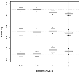
$\nu=1.61$	$\nu=\infty$

Figure 2: Boxplots of estimated baseline survivor probabilities evaluated at the true 90th, 50th, and 10th percentile times, respectively (such that the true probabilities are 0.1, 0.5, and 0.9), vertically stacked for each of four fitted models indicated by the $x$-axis labels.

We now consider model fit by inspecting the estimated baseline survivor curves, i.e., the survivor curve for an individual with $X=0$ which we denote by $S_{0}(t)$. In particular, we focus on this estimated baseline survivor function evaluated at three true quantiles, namely, $Q_{0}(u)$, $u=0.1,0.5,0.9$, since $\hat{S}_{0}(Q_{0}(u))$ is an estimate of the probability $1-u$. Boxplots of these estimates over simulation replicates arising from the true model, $M(\tau,\alpha)$, and the misspecified model, $M(\beta,\alpha)$, are shown in Figure 2. We also display the estimates from two simpler (misspecified) models, $M(\tau)$ and $M(\beta)$, wherein $X$ has been dropped from the $\alpha$ component (specifically, $\alpha_{1}$ is set to zero in these simpler models). Clearly both $M(\tau,\alpha)$ and $M(\beta,\alpha)$ fit the data very well (apart from a little bias in $M(\beta,\alpha)$ when $\nu=\infty$), i.e., the choice of using a $\tau$ or $\beta$ regression component does not alter the model fit much (again mirroring the findings of Section 4.1). On the other hand, when the $\alpha$ regression is dropped, the quality of the model fit decreases considerably as this represents a model misspecification in a much stronger sense than switching from $M(\tau,\alpha)$ to $M(\beta,\alpha)$.

5 Data Analysis

5.1 Lung Cancer

We now consider our modelling framework in the context of a lung cancer study which was the subject of a 1995 Queen’s University Belfast PhD thesis by P. Wilkinson (see Burke and MacKenzie, (2017)). This study concerns 855 individuals who were diagnosed with lung cancer between 1st October 1991 and 30th September 30 1992, who were then followed up until 30th May 1993 (approximately 20% of survival times were right-censored). The main aim of this study was to investigate differences between the following treatment groups: palliative care, surgery, chemotherapy, radiotherapy, and a combined treatment of chemotherapy and radiotherapy. In our analysis we take palliative care (which is a non-curative treatment providing pain relief) as the reference category. Note that, while various other covariates were captured for each individual, our main aim here is to explore the flexibility of our general modelling scheme in the context of the treatment variable.

As discussed in Section 3, we advocate the use of $M(\beta,\alpha)$ and $M(\tau,\alpha)$ since they offer a flexible extension of the popular PH and AFT models (i.e., $M(\beta)$ and $M(\tau)$, respectively) in which the $\alpha$ coefficients indicate non-PH/non-AFT effects (see Section 3.2), and where the baseline distribution is selected via the parameter $\nu_{0}=\log(\kappa+1)$. Thus, we fitted these two models, and their simpler PH and AFT counterparts, to the lung cancer data. We also fitted $M(\beta,\nu)$ and $M(\tau,\nu)$ for comparison, albeit we have argued in Section 3.2 that these are perhaps somewhat less natural. These six fitted models are summarised in Table 5.

We immediately see that the largest AIC/BIC values are associated with the simpler single component (i.e., $\tau$ and $\beta$ only) models which suggests that these models are not sufficiently flexible to capture the more complex non-PH/non-AFT effects observed here. Although, in this particular application, the AFT ($\tau$ only) model has lower AIC/BIC values than that of the PH ($\beta$ only) model, the fit can be greatly improved by modelling shape (either $\alpha$ or $\nu$) in addition to scale. Although the best-fitting model here is $M(\beta,\nu)$, the difference is negligible compared with the models we favour, $M(\beta,\alpha)$ and $M(\tau,\alpha)$. Interestingly, these latter two models have very close AIC/BIC values, indicating that the choice of $\tau$ or $\beta$ component is not at all important here (in line with the findings of Section 4.2). The use of more than two regression components did not yield further improvements in fit (models not shown), and, moreover, estimation of such models tends to be unstable — particularly, of course, those with two scale regression components (see also Section 4). Note that we have also avoided shape-only regression models, i.e., $M(\alpha)$, $M(\nu)$, and $M(\alpha,\nu)$, as, typically, models without scale components are not of interest, and, as we would expect, these models fit the current data very poorly indeed (with $\Delta_{\text{AIC}}>600$).

Table 5: Summary of models fitted to lung cancer data

Model	$M(\beta)$	$M(\tau)$	$M(\beta,\alpha)$	$M(\tau,\alpha)$	$M(\beta,\nu)$	$M(\tau,\nu)$
$\dim(\theta)$	7	7	11	11	11	11
$\ell(\hat{\theta})$	-1956.5	-1943.5	-1927.0	-1926.6	-1925.9	-1930.3
$\Delta_{\text{AIC}}$	53.1	27.2	2.2	1.5	0.0	8.9
$\Delta_{\text{BIC}}$	34.1	8.2	2.2	1.5	0.0	8.9
$\ell(\hat{\theta})$, the value of the log-likelihood; $\dim(\theta)$, the dimension of the model, i.e., number of parameters; $\Delta_{\text{AIC}}$, the AIC values for each model minus AIC${}_{M(\beta,\nu)}=3873.8$ (the lowest AIC in the set); $\Delta_{\text{BIC}}$, analogous to $\Delta_{\text{AIC}}$ where the lowest BIC is BIC${}_{M(\beta,\nu)}=3926.1$.

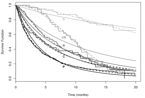
Figure 3: Kaplan-Meier survivor curves (step, solid) for lung cancer treatment groups (P = palliative, C = chemotherapy, R = radiotherapy, CR = chemotherapy and radiotherapy, and S = surgery) with fitted curves overlayed for $M(\beta)$ (solid), $M(\beta,\alpha)$ (dashed), and $M(\beta,\nu)$ (dotted).

We now consider the PH-APGW model, $M(\beta)$, and the two associated shape-regression extensions, $M(\beta,\alpha)$ and $M(\beta,\nu)$, in more detail. The advantage, in terms of model fit, of shape regression components is clear from Figure 3, while the $M(\beta,\alpha)$ and $M(\beta,\nu)$ models themselves are virtually indistinguishable. Table 6 displays the estimated regression coefficients. We can see that both $M(\beta)$ and $M(\beta,\alpha)$ suggest a baseline distribution which is between a log-logistic ($\nu=0$) and a Weibull ($\nu=0.69$), while $M(\beta,\nu)$ assumes a separate baseline distribution for each treatment group. Interestingly, in all three models, all shape parameters ($\nu$ and $\alpha$) are positive which indicates that the hazards are increasing with time in each treatment group (Table 1). While all three models are in agreement when it comes to the overall effectiveness of each treatment as viewed in terms of the scale coefficients (albeit the chemotherapy effect is only statistically significant in $M(\beta)$), the positive shape coefficients in $M(\beta,\alpha)$ suggest that the effectiveness of each treatment reduces to some extent over time (see Section 3.2) – especially in the case of the combined treatment of chemotherapy and radiotherapy.

Table 6: Selected lung cancer models

	Model$(\beta)$		Model$(\beta,\alpha)$				Model$(\beta,\nu)$
	Scale		Scale		Shape		Scale		Shape
Intercept	-1.40	(0.08)	-1.13	(0.09)	0.12	(0.07)	-1.04	(0.10)	0.21	(0.06)
Palliative	0.00	—	0.00	—	0.00	—	0.00	—	0.00	—
Surgery	-2.18	(0.23)	-4.77	(0.97)	1.06	(0.28)	-3.96	(0.66)	0.55	(0.15)
Chemo	-0.38	(0.17)	-0.55	(0.33)	0.13	(0.18)	-0.60	(0.36)	0.11	(0.13)
Radio	-0.56	(0.09)	-1.46	(0.21)	0.52	(0.11)	-1.48	(0.19)	0.36	(0.06)
C$+$R	-0.86	(0.20)	-5.13	(0.96)	1.50	(0.22)	-3.57	(0.60)	0.82	(0.13)
$\hat{\alpha}_{0}$	0.15	(0.08)	$\ast$				0.27  (0.07)
$\hat{\nu}_{0}$	0.46	(0.06)	0.35  (0.05)				$\ast$
The $\ast$ symbol indicates that the shape parameter already appears as the intercept in the shape regression component.

The hazard ratios for the models in Table 6 are shown in Figure 4 where those of $M(\beta,\alpha)$ and $M(\beta,\nu)$ are quite similar. They suggest that while the various treatments reduce the hazard in the first few months, their effect is weakened over time and, perhaps, even become inferior to palliative care in the longer term (however, note that very few individuals remain in the sample beyond 15 months). Clearly SPR models, such as $M(\beta)$, cannot account for covariate effects of this sort.

It is worth highlighting the fact that the basic findings here are qualitatively similar to those of Burke and MacKenzie, (2017) who analysed this lung cancer dataset using $M_{\kappa=1}(\beta,\alpha)$, i.e., a Weibull MPR model. However, the framework of the current paper permits us to consider a much wider range of model structures and distributions in which $M_{\kappa=1}(\beta,\alpha)$ appears as a special case. In particular, $M(\beta,\alpha)$ from Table 6 yields a 95% confidence interval for $\kappa$, $[0.28,0.57]$, which does not support the Weibull ($\kappa=1$) baseline distribution. Furthermore, $\text{AIC}_{M_{\kappa=1}(\beta,\alpha)}-\text{AIC}_{M(\beta,\alpha)}=57.6$, and we can confirm that the improvement in quality of fit is most evident in the palliative care group (which $M_{\kappa=1}(\beta,\alpha)$ does not capture so well). Thus, although the basic findings are unaltered in this particular application, the APGW MPR approach yields a better solution in which uncertainty in selecting the baseline distribution is accounted for. Of course, the APGW MPR model will readily adapt to other applications which might differ significantly (both qualitatively and quantitatively) from $M_{\kappa=1}(\beta,\alpha)$.

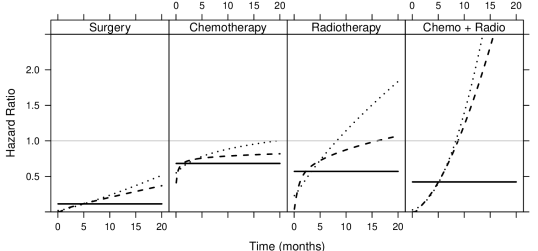
Figure 4: Hazard ratios for each lung cancer treatment relative to palliative care for $M(\beta)$ (solid), $M(\beta,\alpha)$ (dashed), and $M(\beta,\nu)$ (dotted). Line of equality (grey) also shown.

5.2 Melanoma

The Eastern Cooperative Oncology Group (ECOG) trial “EST 1684” was a randomized controlled trial to investigate the adjuvant (i.e., post-surgery) chemotherapy drug “IFN$\alpha$-2b” in treating melanoma (Kirkwood et al.,, 1996). The outcome variable was relapse-free survival, i.e., time from randomization until the earlier of cancer relapse or death. Patients were recruited to the study between 1984 and 1990, and the study ended in 1993. In total, 284 patients were recruited of which 140 were assigned to the control group, and 144 were assigned to the treatment group. This dataset is available in the R package smcure (Chao et al.,, 2012), and variations of it have appeared in the cure model literature (Chen et al.,, 1999; Ibrahim et al.,, 2001).

As in Section 5.1, we fitted the following models: $M(\beta)$, $M(\tau)$, $M(\beta,\alpha)$, $M(\tau,\alpha)$, $M(\beta,\nu)$, and $M(\tau,\nu)$; the results are summarised in Table 7. In this case, the two-component models do not provide a large improvement over the one-component models, and $M(\tau)$ has the lowest AIC and the second-lowest BIC ($M(\tau,\nu)$ has the lowest BIC); the AIC and BIC values for $M(\beta)$ are not much larger than for $M(\tau)$. The models $M(\beta)$, $M(\tau)$, and $M(\tau,\nu)$ are compared to the Kaplan-Meier (KM) curves in Figure 5. The fitted $M(\beta)$ and $M(\tau,\nu)$ curves are similar, and are close to the KM curves. The fitted $M(\tau)$ curves converge later in time, which, visually, look worse compared to the KM curves. However, note that there is very little data in the right tail so that converging curves are plausible when viewed with the level of uncertainty in the tail.

Table 7: Summary of models fitted to melanoma data

Model	$M(\beta)$	$M(\tau)$	$M(\beta,\alpha)$	$M(\tau,\alpha)$	$M(\beta,\nu)$	$M(\tau,\nu)$
$\dim(\theta)$	4	4	5	5	5	5
$\ell(\hat{\theta})$	-368.8	-368.0	-367.7	-367.9	-368.2	-366.6
$\Delta_{\text{AIC}}$	2.4	0.8	2.1	2.6	3.2	0.0
$\Delta_{\text{BIC}}$	1.6	0.0	5.0	5.5	6.1	2.9
$\ell(\hat{\theta})$, the value of the log-likelihood; $\dim(\theta)$, the dimension of the model, i.e., number of parameters; $\Delta_{\text{AIC}}$, the AIC values for each model minus AIC${}_{M(\tau,\nu)}=743.2$ (the lowest AIC in the set); $\Delta_{\text{BIC}}$, analogous to $\Delta_{\text{AIC}}$ where the lowest BIC is BIC${}_{M(\tau)}=758.6$.

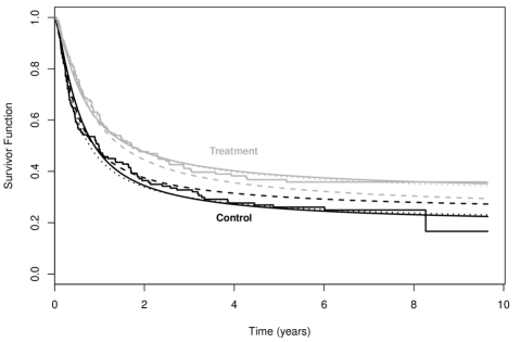
Figure 5: Kaplan-Meier survivor curves (step, solid) for melanoma control and treatment groups with fitted curves overlayed for $M(\beta)$ (solid), $M(\tau)$ (dashed), and $M(\tau,\nu)$ (dotted).

The parameter estimates for $M(\beta)$, $M(\tau)$, and $M(\tau,\nu)$ are shown in Table 8. Firstly note that the scale coefficient of treatment is negative which indicates that treatment improves survival. Furthermore, for $M(\beta)$ and $M(\tau)$, note that the parameter $\kappa=\exp(\nu_{0})-1$ is negative, and, similarly, for $M(\tau,\nu)$, the estimated $\kappa$ is negative in each treatment group. Thus, all three models point towards a cure proportion. The fact that the power shape parameter, $\gamma=\exp(\alpha)$, is greater than one for all three models means that the hazard function has an up-then-down shape. This type of hazard function is commonly observed in the cure literature since the population becomes increasingly composed of cured individuals (i.e., zero hazard) over time.

Table 8: Selected melanoma models

	Model$(\beta)$		Model$(\tau)$		Model$(\tau,\nu)$
	Scale		Scale		Scale		Shape
Intercept	0.60	(0.16)	0.65	(0.14)	0.67	(0.15)	-0.45	(0.05)
Control	0.00	—	0.00	—	0.00	—	0.00	—
Treatment	-0.36	(0.14)	-0.52	(0.20)	-0.53	(0.19)	-0.14	(0.08)
$\hat{\alpha}_{0}$	0.36	(0.07)	0.44	(0.08)	0.45  (0.08)
$\hat{\nu}_{0}$	-0.73	(0.11)	-0.51	(0.05)	$\ast$
The $\ast$ symbol indicates that the shape parameter already appears as the intercept in the shape regression component.

Table 9: Estimated melanoma cure proportions with 95% confidence intervals

Model	Treatment	Control	Difference
$M(\beta)$	0.30 (0.21,0.39)	0.18 (0.10,0.26)	0.12 (0.03,0.21)
$M(\tau)$	0.22 (0.15,0.30)	$=$ Treatment	—
$M(\tau,\nu)$	0.24 (0.18,0.39)	0.11 (0.09,0.27)	0.12 (-0.02,0.23)
$p_{\text{Difference}}=p_{\text{Treatment}}-p_{\text{control}}$.

When $-1<\kappa<0$, the APGW-MPR cure proportion is given by$\exp\{\lambda(\kappa+1)/\kappa\}>0$, i.e., the cure proportion depends on $\kappa$ and $\lambda$. Therefore, $M(\beta)$ and $M(\tau,\nu)$ suggest that the cure proportion depends on treatment, while $M(\tau)$ suggests that it does not. The estimated cure proportions, along with 95% confidence intervals, are shown in Table 9. Had we fixed to a log-logistic baseline (i.e., $\kappa=0$), the resulting $M_{\kappa=0}(\beta)$ and $M_{\kappa=0}(\tau)$ models (not shown) provide an extremely poor fit to the data. This is noteworthy as even the heaviest-tail non-cure APGW model is not supported by the data (and, of course, a Weibull baseline is worse still). The heaviness of tail here can only be supported within the APGW family by a cure model.

6 Discussion

Our proposed APGW-MPR modelling framework is highly flexible and can adapt readily to a wide variety of applications in survival analysis and reliability. In particular, this framework includes the practically important AFT and PH models, and generalises them through shape regression components. Furthermore, the APGW baseline model covers the primary shapes of hazard function (constant, increasing, decreasing, up-then-down, down-then-up) within some of the most popular survival distributions (log-logistic, Burr type XII, Weibull, Gompertz) using only two shape parameters.

In practice, the full four-component APGW-MPR model is likely to be more flexible than is required for most purposes. In fact, we suggest that covariates should appear via just one scale-type component ($\tau$ or $\beta$), along with the $\alpha$ shape component which permits survivor functions with differing shapes and indicates departures from more basic AFT or PH effects, while $\nu=\log(\kappa+1)$ is a covariate-independent parameter which allows us to choose among distributions within one unified framework. We have found that the scale-type parameters ($\tau$ and $\beta$) are highly intertwined in the sense that they cannot be estimated simultaneously within the same model reliably, and are highly correlated. This is true across the full range of distributions (varying $\nu$), going well beyond the well-known Weibull case in which the two scale components are equivalent. The implication of this is that, in terms of performance gain, the movement from AFT to PH modelling (or vice versa) might not be very large, whereas we have found that modelling the shape is a more fruitful alteration to the regression specification.

Finally, the perspective of this paper has been to investigate survival modelling generally, to cover some of the most popular models, and to discover some of the better modelling choices that can be made within this framework. Although we have developed these ideas in a fully parametric context, non-parametric equivalents, while possible, are beyond the scope of the present paper (but are investigated in a separate line of work (Burke et al.,, 2018)). However, it is worth highlighting that perhaps too much emphasis is placed on non-/semi-parametric approaches in survival analysis whereby undue weight is attached to the flexibility of the baseline distribution in comparison to the flexibility of its regression structure. Our general approach to survival modelling provides a framework within which one can consider the most important components of survival modelling (including which might potentially be modelled non-parametrically), and we believe that this insight can lead to better modelling practice in general.

Appendix

Appendix A The (A)PGW Distribution as a Transformation Model

Linear transformation models (c.f. Kalbfleisch and Prentice, (2002, sec. 7.5); Zeng and Lin, (2007)) are concerned with c.h.f.’s of the form

$$H_{T}(t)=w(\theta H_{0}(t))$$ (A:1)

where $\theta>0$ depends log-linearly on covariates and both the transformation function $w$ and baseline function $H_{0}$ are c.h.f.’s. It is easy to see that the (A)PGW c.h.f.’s $H_{N}$ and $H_{A}$ are of the form (A:1). Either is a transformation model with $H_{0}$ the Weibull c.h.f. $t^{\gamma}$; in terms of the overall model, whenever the Weibull is used as baseline, $\theta^{-1/\gamma}$ is the horizontal scale parameter so that when covariates are included only in it, the transformation model is an accelerated failure time model. The transformation $w$ is a version of the Box-Cox transformation given, in the simpler case of $H_{N}$, by $w(y)=(1+y)^{\kappa}-1$ (Box and Cox,, 1964; Yeo and Johnson,, 2000).

If $Y$ is the lifetime random variable following the transformation model with, for simplicity, c.h.f. $H_{N}$, then the model can also be written in the form $\gamma\log Y=-\log\theta+\log E$ where $E$ follows the distribution with c.h.f.  $(1+y)^{\kappa}-1$.

Appendix B Simulation Studies with Smaller Samples

This section displays analogous results to those of Table 4 from the main paper but for $n=500$ and $n=100$ respectively.

Table 10: Median and standard error (in brackets) of estimates when $n=500$

	Model$(\tau,\beta,\alpha)$
$\nu$	$\hat{\tau}_{0}$		$\hat{\tau}_{1}$		$\hat{\beta}_{0}$		$\hat{\beta}_{1}$		$\hat{\alpha}_{0}$		$\hat{\alpha}_{1}$		$\hat{\nu}_{0}$
0.00	1.06	(1.57)	0.57	(1.63)	-0.25	(1.73)	0.01	(1.13)	0.23	(0.21)	-0.49	(0.32)	0.07	(1.02)
0.22	1.30	(1.62)	0.45	(2.66)	-0.52	(1.95)	0.21	(2.13)	0.27	(0.24)	-0.53	(0.37)	0.27	(0.73)
0.41	1.05	(1.73)	0.81	(3.17)	-0.19	(2.11)	-0.03	(2.72)	0.27	(0.24)	-0.50	(0.34)	0.35	(0.78)
0.69	0.88	(2.12)	0.45	(4.19)	-0.15	(2.60)	0.19	(3.70)	0.21	(0.26)	-0.51	(0.28)	0.65	(4.26)
1.10	0.43	(1.51)	0.26	(2.93)	0.33	(1.91)	0.04	(2.72)	0.15	(0.16)	-0.49	(0.23)	1.53	(7.11)
1.61	0.53	(1.09)	0.40	(1.98)	0.25	(1.47)	-0.01	(2.03)	0.19	(0.16)	-0.50	(0.24)	14.75	(7.06)
$\infty$	0.91	(0.72)	0.68	(1.26)	-0.15	(1.07)	-0.02	(1.41)	0.19	(0.16)	-0.51	(0.24)	15.43	(6.48)
	Model$(\tau,\alpha)$
$\nu$	$\hat{\tau}_{0}$		$\hat{\tau}_{1}$		$\hat{\beta}_{0}$		$\hat{\beta}_{1}$		$\hat{\alpha}_{0}$		$\hat{\alpha}_{1}$		$\hat{\nu}_{0}$
0.00	0.79	(0.13)	0.60	(0.19)	0.00	—	0.00	—	0.20	(0.09)	-0.50	(0.09)	0.00	(0.09)
0.22	0.80	(0.12)	0.59	(0.16)	0.00	—	0.00	—	0.20	(0.09)	-0.50	(0.09)	0.22	(0.13)
0.41	0.79	(0.12)	0.58	(0.15)	0.00	—	0.00	—	0.20	(0.09)	-0.50	(0.08)	0.42	(0.18)
0.69	0.80	(0.13)	0.58	(0.14)	0.00	—	0.00	—	0.20	(0.09)	-0.50	(0.08)	0.72	(0.30)
1.10	0.79	(0.13)	0.60	(0.12)	0.00	—	0.00	—	0.20	(0.09)	-0.51	(0.09)	1.13	(1.73)
1.61	0.80	(0.11)	0.60	(0.11)	0.00	—	0.00	—	0.20	(0.09)	-0.50	(0.09)	1.62	(4.26)
$\infty$	0.84	(0.07)	0.62	(0.08)	0.00	—	0.00	—	0.24	(0.08)	-0.51	(0.09)	13.84	(6.97)
	Model$(\beta,\alpha)$
$\nu$	$\hat{\tau}_{0}$		$\hat{\tau}_{1}$		$\hat{\beta}_{0}$		$\hat{\beta}_{1}$		$\hat{\alpha}_{0}$		$\hat{\alpha}_{1}$		$\hat{\nu}_{0}$
0.00	0.00	—	0.00	—	0.88	(0.16)	0.03	(0.12)	0.17	(0.08)	-0.51	(0.08)	-0.35	(0.18)
0.22	0.00	—	0.00	—	0.91	(0.17)	0.04	(0.11)	0.19	(0.08)	-0.51	(0.08)	-0.07	(0.23)
0.41	0.00	—	0.00	—	0.94	(0.18)	0.04	(0.12)	0.19	(0.08)	-0.51	(0.08)	0.22	(0.30)
0.69	0.00	—	0.00	—	0.98	(0.20)	0.07	(0.14)	0.20	(0.09)	-0.50	(0.09)	0.72	(0.94)
1.10	0.00	—	0.00	—	1.04	(0.17)	0.08	(0.15)	0.22	(0.08)	-0.50	(0.09)	1.74	(5.10)
1.61	0.00	—	0.00	—	1.20	(0.15)	0.09	(0.17)	0.27	(0.07)	-0.49	(0.10)	14.00	(7.03)
$\infty$	0.00	—	0.00	—	1.54	(0.15)	0.12	(0.20)	0.37	(0.08)	-0.49	(0.10)	16.85	(1.76)
All numbers are rounded to two decimal places. For the models with fixed parameters, the “estimated” value shown is the value at which the parameter is fixed, and its standard error is then indicated by “—”.

Table 11: Median and standard error (in brackets) of estimates when $n=100$

	Model$(\tau,\beta,\alpha)$
$\nu$	$\hat{\tau}_{0}$		$\hat{\tau}_{1}$		$\hat{\beta}_{0}$		$\hat{\beta}_{1}$		$\hat{\alpha}_{0}$		$\hat{\alpha}_{1}$		$\hat{\nu}_{0}$
0.00	1.32	(2.72)	0.88	(2.91)	-0.49	(3.18)	-0.01	(1.97)	0.39	(0.43)	-0.52	(0.63)	0.08	(2.53)
0.22	1.29	(2.21)	0.85	(3.20)	-0.39	(2.74)	0.01	(2.39)	0.38	(0.42)	-0.49	(0.56)	0.17	(3.18)
0.41	1.10	(1.85)	0.83	(3.21)	-0.22	(2.24)	0.02	(2.73)	0.35	(0.44)	-0.51	(0.52)	0.24	(3.41)
0.69	0.87	(1.94)	0.67	(3.47)	-0.14	(2.48)	-0.03	(3.12)	0.21	(0.45)	-0.49	(0.46)	0.87	(6.34)
1.10	0.61	(1.52)	0.50	(2.84)	0.05	(1.96)	-0.02	(2.69)	0.17	(0.33)	-0.52	(0.37)	12.66	(7.62)
1.61	0.70	(1.22)	0.57	(2.46)	0.05	(1.72)	0.05	(2.52)	0.17	(0.28)	-0.52	(0.37)	15.31	(7.02)
$\infty$	0.89	(0.89)	0.75	(1.81)	-0.16	(1.44)	-0.14	(2.05)	0.23	(0.26)	-0.53	(0.34)	15.95	(6.12)
	Model$(\tau,\alpha)$
$\nu$	$\hat{\tau}_{0}$		$\hat{\tau}_{1}$		$\hat{\beta}_{0}$		$\hat{\beta}_{1}$		$\hat{\alpha}_{0}$		$\hat{\alpha}_{1}$		$\hat{\nu}_{0}$
0.00	0.79	(0.29)	0.59	(0.44)	0.00	—	0.00	—	0.24	(0.20)	-0.50	(0.20)	-0.02	(0.27)
0.22	0.79	(0.28)	0.58	(0.39)	0.00	—	0.00	—	0.21	(0.20)	-0.50	(0.21)	0.22	(1.47)
0.41	0.76	(0.27)	0.58	(0.35)	0.00	—	0.00	—	0.21	(0.20)	-0.51	(0.20)	0.45	(1.93)
0.69	0.79	(0.26)	0.58	(0.31)	0.00	—	0.00	—	0.22	(0.20)	-0.51	(0.20)	0.72	(3.68)
1.10	0.82	(0.24)	0.59	(0.25)	0.00	—	0.00	—	0.24	(0.20)	-0.51	(0.20)	1.07	(5.51)
1.61	0.83	(0.20)	0.63	(0.24)	0.00	—	0.00	—	0.26	(0.19)	-0.52	(0.19)	1.54	(6.86)
$\infty$	0.89	(0.16)	0.66	(0.19)	0.00	—	0.00	—	0.30	(0.18)	-0.50	(0.21)	4.00	(7.52)
	Model$(\beta,\alpha)$
$\nu$	$\hat{\tau}_{0}$		$\hat{\tau}_{1}$		$\hat{\beta}_{0}$		$\hat{\beta}_{1}$		$\hat{\alpha}_{0}$		$\hat{\alpha}_{1}$		$\hat{\nu}_{0}$
0.00	0.00	—	0.00	—	0.89	(0.36)	0.04	(0.25)	0.19	(0.17)	-0.51	(0.17)	-0.34	(0.44)
0.22	0.00	—	0.00	—	0.89	(0.38)	0.07	(0.28)	0.19	(0.18)	-0.50	(0.18)	0.01	(0.79)
0.41	0.00	—	0.00	—	0.92	(0.38)	0.03	(0.30)	0.19	(0.19)	-0.51	(0.19)	0.24	(1.99)
0.69	0.00	—	0.00	—	1.04	(0.38)	0.06	(0.33)	0.23	(0.17)	-0.51	(0.19)	0.70	(3.81)
1.10	0.00	—	0.00	—	1.21	(0.35)	0.07	(0.33)	0.29	(0.16)	-0.50	(0.20)	1.27	(5.92)
1.61	0.00	—	0.00	—	1.35	(0.36)	0.09	(0.38)	0.34	(0.17)	-0.50	(0.21)	2.32	(7.23)
$\infty$	0.00	—	0.00	—	1.66	(0.36)	0.13	(0.43)	0.42	(0.17)	-0.50	(0.22)	15.98	(6.32)
All numbers are rounded to two decimal places. For the models with fixed parameters, the “estimated” value shown is the value at which the parameter is fixed, and its standard error is then indicated by “—”.

References

- Bagdonaviçius and Nikulin, (2002) Bagdonaviçius, V. and Nikulin, M. (2002). Accelerated Life Model; Modeling and Statistical Analysis. Chapman & Hall/CRC, Boca Raton, FL.
- Box and Cox, (1964) Box, G. and Cox, D. (1964). An analysis of transformations (with discussion). Journal of the Royal Statistical Society Series B, 26:211–252.
- Burke et al., (2018) Burke, K., Eriksson, F., and Pipper, C. B. (2018). Semiparametric multi-parameter regression survival modelling. Submitted.
- Burke and MacKenzie, (2017) Burke, K. and MacKenzie, G. (2017). Multi-parameter regression survival modelling: An alternative to proportional hazards. Biometrics, 73:678–686.
- Chao et al., (2012) Chao, C., Yubo, Z., Yingwei, P., and Jiajia, Z. (2012). smcure: fit semiparametric mixture cure models. R package version 2.0.
- Chen et al., (1999) Chen, M., Ibrahim, J., and Sinha, D. (1999). A new Bayesian model for survival data with a surviving fraction. J. Am. Statist. Ass., 94:909–919.
- Chen and Jewell, (2001) Chen, Y. and Jewell, N. (2001). On a general class of semiparametric hazards regression models. Biometrika, 88:687–702.
- Chen, (2000) Chen, Z. (2000). A new two-parameter lifetime distribution with bathtub shape or increasing failure rate function. Statistical Probability Letters, 49:155–161.
- Cox and Matheson, (2014) Cox, C. and Matheson, M. (2014). A comparison of the generalized gamma and exponentiated Weibull distributions. Statistics in Medicine, 33:3772–3780.
- Dimitrakopoulou et al., (2007) Dimitrakopoulou, T., Adamidis, K., and Loukas, S. (2007). A lifetime distribution with an upside-down bathtub-shaped hazard function. IEEE Transactions on Reliability, 56:308–311.
- Ibrahim et al., (2001) Ibrahim, J., Chen, M., and Sinha, D. (2001). Bayesian semiparametric models for survival data with a cure fraction. Biometrics, 57:383–388.
- Jones and Noufaily, (2015) Jones, M. and Noufaily, A. (2015). Log-location-scale-log-concave distributions for survival and reliability analysis. Electronic Journal of Statistics, 9:2732–2750.
- Jones et al., (2018) Jones, M., Noufaily, A., and Burke, K. (2018). A bivariate power generalized Weibull distribution: a flexible parametric model for survival analysis. Submitted.
- Kalbfleisch and Prentice, (2002) Kalbfleisch, J. and Prentice, R. (2002). The Statistical Analysis of Failure Time Data. Wiley, Hoboken, NJ., 2 edition.
- Kirkwood et al., (1996) Kirkwood, J., Strawderman, M., Ernstoff, M., Smith, T., Borden, E., and Blum, R. (1996). Interferon alfa-2b adjuvant therapy of high-risk resected cutaneous melanoma: the Eastern Cooperative Oncology Group Trial EST 1684. J. Clinical Oncology, 14:7–17.
- Matheson et al., (2017) Matheson, M., Muñoz, A., and Cox, C. (2017). Describing the flexibility of the generalized gamma and related distributions. Journal of Statistical Distributions and Applications, 4:Article 15.
- Nadarajah and Haghighi, (2011) Nadarajah, S. and Haghighi, F. (2011). An extension of the exponential distribution. Statistics, 45:543–558.
- Nikulin and Haghighi, (2009) Nikulin, M. and Haghighi, F. (2009). On the power generalized Weibull family: model for cancer censored data. Metron, 67:75–86.
- Tsodikov et al., (2003) Tsodikov, A., Ibrahim, J., and Yakovlev, A. (2003). Estimating cure rates from survival data: an alternative to two-component mixture models. Journal of the American Statistical Association, 98:1063–1078.
- Xie et al., (2002) Xie, M., Tang, Y., and Goh, T. (2002). A modified Weibull extension with bathtub-shaped failure rate function. Reliability Engineering and System Safety, 73:279–285.
- Yeo and Johnson, (2000) Yeo, I. and Johnson, R. (2000). A new family of power transformations to improve normality or symmetry. Biometrika, 87:954–959.
- Zeng and Lin, (2007) Zeng, Z. and Lin, D. (2007). Maximum likelihood estimation in semiparametric regression models with censored data (with discussion). Journal of the Royal Statistical Society Series B, 69:507–564.