Abstract

We are concerned with the flexible parametric analysis of bivariate survival data. Elsewhere, we have extolled the virtues of the “power generalized Weibull” (PGW) distribution as an attractive vehicle for univariate parametric survival analysis: it is a tractable, parsimonious, model which interpretably allows for a wide variety of hazard shapes and, when adapted (to give an adapted PGW, or APGW, distribution), covers a wide variety of important special/limiting cases. Here, we additionally observe a frailty relationship between a PGW distribution with one value of the parameter which controls distributional choice within the family and a PGW distribution with a smaller value of the same parameter. We exploit this frailty relationship to propose a bivariate shared frailty model with PGW marginal distributions: these marginals turn out to be linked by the so-called BB9 or “power variance function” copula. This particular choice of copula is, therefore, a natural one in the current context. We then adapt the bivariate PGW distribution, in turn, to accommodate APGW marginals. We provide a number of theoretical properties of the bivariate PGW and APGW models and show the potential of the latter for practical work via an illustrative example involving a well-known retinopathy dataset, for which the analysis proves to be straightforward to implement and informative in its outcomes. The novelty in this article is in the appropriate combination of specific ingredients into a coherent and successful whole.

Keywords: BB9 copula; Gompertz; log-logistic; power variance frailty; shared frailty.

1. Introduction

In this article, we are concerned with the flexible parametric analysis of paired survival data. Such data arise frequently in medicine, for example, when comparing treatment and control on pairs of related sampling units such as an individual’s eyes or limbs, or when measurements are made pre- and post-intervention of some kind, or when familial data such as observations made on twins or on a parent and child are of interest, and so on. Here, our concern is with providing a flexible parametric model for the entire, correlated, bivariate distribution of the pairs of outcomes. To do so, we reason for specific elements and combine them into a new overall model in a coherent and successful way.

In Burke, Jones & Noufaily (2018; henceforth BJN), we argued, in the univariate case, in favour of flexible parametric survival analysis in general and for the use of an adapted form of an existing flexible parametric model called the “power generalized Weibull” (PGW) distribution in particular. Advantages of the latter include that its two shape parameters control key shapes of the hazard function (constant, increasing, decreasing, up-then-down, down-then-up, and no others) and that, when adapted, several common and important survival distributions are special/limiting cases of it (log-logistic, Weibull, Gompertz and others). The PGW distribution is one of only a very few to parsimoniously and interpretably control hazard shapes as just described — others include the generalized gamma (GG) and exponentiated Weibull (EW) distributions — but it is preferred by us because of its extra tractability and its greater breadth of particular cases.

In this article, we also take advantage of a further feature of the PGW distribution not shared with GG or EW distributions. Inter alia, in Section 2.1, we obtain a frailty relationship between a PGW distribution with one value of the parameter $\kappa$ which controls specific distributional choice within the PGW family and a smaller value of the same parameter. We then exploit this frailty relationship and first pursue — in Section 3 — a natural extension of the PGW distribution, to the multivariate case in principle, but more specifically, for convenience and many practical applications, to the bivariate case, through the shared frailty route. In Section 4, we build on the work of Section 3 to provide a closely related bivariate distribution with adapted PGW (APGW) marginals, which is the version that we suggest for practical work, as exemplified in Section 5. The distribution has eight basic parameters, and these can be extended in natural ways to accommodate covariates. Even so, the model proves to be straightforward to implement using maximum likelihood techniques, and to provide interpretable and insightful analysis of the example on which we illustrate the methodology.

In more detail, we first provide the relevant univariate background in Section 2, including the univariate frailty result that drives the remainder of the paper in Section 2.1. The bivariate PGW distribution of interest in this article is then developed in Section 3.1: its conditional hazard functions are considered in Section 3.2, its cross ratio dependence function in Section 3.3, and its copula representation, and properties ensuing therefrom, in Section 3.4. After explaining why we cannot follow the same shared frailty approach for the APGW distribution as we do for the PGW distribution, we propose a bivariate APGW distribution by transforming PGW marginal distributions to APGW marginal distributions, retaining the same copula; see Section 4.1. Properties other than those solely dependent on the copula, which are the same for both bivariate PGW and APGW distributions, are considered in Section 4.2. We provide an illustrative example of the application of the APGW distribution to a standard, retinopathy, dataset in Section 5, first without its covariate (Section 5.1) and then with the inclusion of the covariate (Section 5.2). In particular, we observe how much the choice of marginal distributions impacts on the degree of dependence of the bivariate failure model. We conclude the article with brief further discussion in Section 6.

As the reader will observe, the distributions of interest in this article retain the high degree of tractability of their univariate counterparts.

2. Univariate background

Write PGW$(\gamma,\kappa,\lambda)$ for the PGW distribution with power parameter $\gamma>0$, distribution-choosing parameter $\kappa>0$ and vertical scale/proportional hazards (PH) parameter $\lambda>0$. That is, it has cumulative hazard function (c.h.f.)

$$\lambda\,H_{N}(t;\gamma,\kappa)=\lambda\left\{(1+t^{\gamma})^{\kappa}-1\right\}.$$

In practice, it is also important to consider a horizontal scale/accelerated failure time (AFT) parameter $\phi>0$ which enters the c.h.f. via $\lambda H_{N}(\phi t;\gamma,\kappa)$; for theoretical purposes, we can set $\phi=1$ without loss of generality. The PGW distribution was first introduced by Bagdonaviçius & Nikulin (2002) (see also Nikulin & Haghighi, 2009), independently re-introduced by Dimitrakopoulou, Adamidis & Loukas (2007), and recognised as an interesting competitor to the GG and EW distributions in Jones & Noufaily (2015).

The shape parameters $\gamma$ and $\kappa$ control the ‘head’ (values near zero) and tail of the distribution in the sense that the hazard function $h_{N}(t;\gamma,\kappa)=H^{\prime}_{N}(t;\gamma,\kappa)$ behaves as $t^{\gamma-1}$ as $t\to 0$ and as $t^{\gamma\kappa-1}$ as $t\to\infty$. This allows a hazard function with a zero, finite or infinite value at its head and likewise, independently, at its tail. What is more, the hazard function joins head to tail in a smooth manner which yields a decreasing hazard when $\gamma\leq 1$ and $\kappa\gamma\leq 1$, an increasing hazard when $\gamma\geq 1$ and $\kappa\gamma\geq 1$, an up-then-down (often called ‘bathtub’) hazard when $\gamma\geq 1$ and $\kappa\gamma\leq 1$, and a down-then-up (sometimes called ‘upside-down bathtub’) hazard when $\gamma\leq 1$ and $\kappa\gamma\geq 1$. If $\gamma=\kappa=1$, the hazard function is constant (the PGW distribution is then the exponential distribution).

BJN principally work with an adapted form of the PGW distribution, written APGW$(\gamma,\kappa,\lambda)$; this has as its c.h.f. a horizontally and vertically rescaled form of the basic PGW c.h.f.:

$$\lambda\,H_{A}(t;\gamma,\kappa)=\lambda\,\left(\frac{\kappa+1}{\kappa}\right)\left\{\left(1+\frac{t^{\gamma}}{\kappa+1}\right)^{\kappa}-1\right\}.$$

Here, $\gamma,\lambda>0$ and $\phi=1$ as before, but the domain of $\kappa$ can be extended (if desired) from $\kappa>0$ to $\kappa>-1$; this affords a cure model when $-1<\kappa<0$, in which the ‘improper’ survival function tends to $\exp\{\lambda(\kappa+1)/\kappa\}$ as $t\to\infty$. Of course, when $\kappa>0$, hazard function shapes, as described above for $h_{N}$, are unaffected.

When $\kappa=1$, (A)PGW distributions are Weibull distributions; when $\kappa=2,$$\gamma=1$, they are linear hazard distributions. The reason for switching from $H_{N}$ to $H_{A}$ is that $H_{A}$ readily accommodates limiting cases, which also turn out to be important and popular survival models: $\kappa=0$ corresponds to the Burr Type XII distribution which incorporates the log-logistic distribution when $\lambda=1$; and when $\kappa\to\infty$, the PGW distribution tends to a form sometimes called the ‘Weibull extension’ model which, for $\gamma=1$, is the Gompertz distribution. The APGW distribution therefore affords, by choice of $\kappa$, a wide range of popular survival models, from light-tailed Gompertz, through the ubiquitous Weibull, to the heavy-tailed log-logistic, and ‘beyond’ to certain cure models.

2.1 Frailty links

Frailty is usually introduced into survival models by mixing over the distribution of the proportionality parameter $B$ say (Hougaard, 2000, Duchateau & Janssen, 2008, Wienke, 2011). A given survival distribution can be produced from another given survival distribution by such frailty mixing if the ratio of their hazard functions is decreasing (Gupta & Gupta, 1996). Thus, when PGW$({\color[rgb]{0,0,0}\gamma,\,\kappa,\,B})$ is mixed with a certain frailty distribution, PGW$({\color[rgb]{0,0,0}\gamma,\,\omega\kappa,\,\lambda})$ for $0\leq\omega\leq 1$ and appropriate $\lambda>0$ results. Notice that the frailty mixing ‘moves us down’ from a PGW distribution with parameter $\kappa$ to a PGW distribution with (the same value of $\gamma$ and) smaller parameter $\omega\kappa$. The following result identifies the mixing distribution. It is a tempered stable (TS), or power variance distribution (Tweedie, 1984, Hougaard, 1986, 2000, Fischer & Jakob, 2016). This distribution has three parameters, $0\leq\omega\leq 1$, $\xi>0$ and $\theta\geq 0$. However, we will take $\theta=1$ throughout and refer to the corresponding distribution as $TS(\omega,\xi)$. It is defined through its Laplace transform given by

$${\cal L}_{\omega,\xi}(s)=\exp\left[{\color[rgb]{0,0,0}\xi\left\{1-(1+s)^{\omega}\right\}/\omega}\right].$$

Result 1. Let $T|B=b\sim\textrm{PGW}({\color[rgb]{0,0,0}\gamma,\,}\kappa,b)$ and let $B\sim\textrm{TS}(\omega,{\color[rgb]{0,0,0}\omega\lambda}).$ Then, $T\sim\textrm{PGW}({\color[rgb]{0,0,0}\gamma,\,\omega\kappa,\,\lambda})$.

Proof. Denote by $g_{\omega,\xi}$ the density of TS$(\omega,{\color[rgb]{0,0,0}\omega\lambda})$. Then,

$$P(T\geq t) = \int_{0}^{\infty}\exp\{-b\,H_{N}(t^{\gamma};\kappa)\}g_{\omega,{\color[rgb]{0,0,0}\omega\lambda}}(b)\,db={\cal L}_{\omega,{\color[rgb]{0,0,0}\omega\lambda}}\{H_{N}(t^{\gamma};\kappa)\}$$

$$= \exp\left({\color[rgb]{0,0,0}\lambda}\left[{\color[rgb]{0,0,0}1-(1+t^{\gamma})^{\kappa\omega}}\right]\right)=\exp\left\{-{\color[rgb]{0,0,0}\lambda}H_{N}(t^{\gamma};\omega\kappa)\right\}.\,\,\,\,\,\,\,\Box$$

Some interesting special cases of Result 1 are that:

• $\omega=1/2$: if $T|B=b\sim\textrm{PGW}({\color[rgb]{0,0,0}\gamma,\,}\kappa,b)$ and $B$ follows the inverse Gaussian distribution with parameters $(1/2,1/2)$, then $T\sim\textrm{PGW}({\color[rgb]{0,0,0}\gamma,\,}\kappa/2,1)$;

• $\omega=0$: if $T|B=b\sim\textrm{PGW}({\color[rgb]{0,0,0}\gamma,\,}\kappa,b)$ and $B$ follows the unit-scale gamma distribution with shape parameter $\xi$, then $T$ follows the Burr Type XII distribution with power parameter $\gamma$ and proportionality parameter $\xi\kappa$. (When $\kappa=1$, this is the well known result that a Weibull distribution with gamma frailty results in the Burr Type XII distribution.)

A related frailty link between the $\kappa=\infty$ and $\kappa=1$ adapted PGW distributions is:

• if $T|B=b$ has c.h.f. $b(e^{t^{\gamma}}-1)$ and $B$ follows the exponential distribution with parameter 1, then $T$ follows the Weibull distribution.

There is a similar, if more complicated, frailty mixing result for the APGW distribution but, because the mixing distribution then depends on $\kappa$, this proves not to be so convenient for extension to the bivariate case. (It is included in Appendix A for completeness.) Instead, we make our bivariate extension based on the original PGW distribution and then change the marginals to APGW distributions, retaining the dependence structure associated with the PGW-based extension.

3. The bivariate shared frailty PGW model

3.1 The model

In the bivariate case, suppose that, for $i=1,2$, $T_{i}|B=b\sim{\rm PGW}(\gamma_{i},\kappa_{i},b)$ independently and $B\sim{\rm TS}(\omega,\omega\lambda)$ with $\lambda>0$ and $0\leq\omega\leq 1$. This is a shared frailty model: given the single, shared, frailty random variable $B=b$, the survival times are (conditionally) independent; the shared frailty introduces the dependence, and this dependence is necessarily positive except for the special case of independence (Hougaard, 2000, Duchateau & Janssen, 2008, Wienke, 2011). In this case, $T_{1}$ and $T_{2}$ are (marginally) independent when $\omega=1$, because then $TS(1,\lambda)$ reduces to a point mass at $\lambda$.

The bivariate survival function can be obtained through an extension of the proof of Result 1. Denote by $g_{\omega,\omega\lambda}$ the density of TS$(\omega,\omega\lambda)$. Then,

$$S_{N}(t_{1},t_{2}) \equiv P(T_{1}\geq t_{1},T_{2}\geq t_{2})$$

$$= \int_{0}^{\infty}P(T_{1}\geq t_{1};\gamma_{1},\kappa_{1},b)\,P(T_{2}\geq t_{2};\gamma_{2},\kappa_{2},b)\,g_{\omega,\omega\lambda}(b)\,db$$

$$= \int_{0}^{\infty}\exp\left[-b\left\{H_{N}(t_{1};\gamma_{1},\kappa_{1})+b\,H_{N}(t_{2};\gamma_{2},\kappa_{2})\right\}\right]\,g_{\omega,\omega\lambda}(b)\,db$$

$$= {\cal L}_{\omega,\omega\lambda}\left\{H_{N}(t_{1};\gamma_{1},\kappa_{1})+H_{N}(t_{2};\gamma_{2},\kappa_{2})\right\}$$

$$= \exp\left(\lambda\left[1-\left\{(1+t_{1}^{\gamma_{1}})^{\kappa_{1}}+(1+t_{2}^{\gamma_{2}})^{\kappa_{2}}-1\right\}^{\omega}\right]\right).$$

The univariate marginals are, of course, $T_{1}\sim{\rm PGW}(\gamma_{1},\omega\kappa_{1},\lambda)$ and $T_{2}\sim\linebreak{\rm PGW}(\gamma_{2},\omega\kappa_{2},\lambda)$, by construction. This suggests reparametrising by $\tau_{i}=\omega\kappa_{i}$, $i=1,2$, in which case

$$S_{N}(t_{1},t_{2})=\exp\left[\lambda\left\{1-L_{N}^{\omega}(t_{1},t_{2})\right\}\right]$$ (1)

where

$$L_{N}(t_{1},t_{2})\equiv(1+t_{1}^{\gamma_{1}})^{\tau_{1}/\omega}+(1+t_{2}^{\gamma_{2}})^{\tau_{2}/\omega}-1,$$ (2)

so that $T_{1}\sim{\rm PGW}(\gamma_{1},\tau_{1},\lambda)$, $T_{2}\sim{\rm PGW}(\gamma_{2},\tau_{2},\lambda)$ and $\omega$ and $\lambda$ control the dependence between $T_{1}$ and $T_{2}$. This is the bivariate model with PGW marginals of interest in this article.

Just once, we mention the multivariate analogue of a result, namely

$$P(T_{1}\geq t_{1},...,T_{p}\geq t_{p})=\exp\left(\lambda\left[1-\left\{\sum_{i=1}^{p}(1+t_{i}^{\gamma_{i}})^{\tau_{i}/\omega}-(p-1)\right\}^{\omega}\right]\right).$$

in order to remind the reader that a multivariate version of our bivariate development is possible, if desired. Indeed, if $\tau_{1}=\tau_{2}=\omega$ in (1), this is a special case (his $\kappa=1$) of the “multivariate distribution with Weibull connections” of Crowder (1989). Its bivariate form is $S_{N;C}(t_{1},t_{2})=\exp\left[\lambda\left\{1-L_{N;C}^{\omega}(t_{1},t_{2})\right\}\right]$ where $L_{N;C}(t_{1},t_{2})\equiv t_{1}^{\gamma_{1}}+t_{2}^{\gamma_{2}}+1.$

3.2 Conditional hazard functions

Returning to the bivariate case, all joint and conditional density, survival and hazard functions are available in closed form. We will explicitly look at two conditional distributions. For ease of notation, write $K(t_{2})=(1+t_{2}^{\gamma_{2}})^{\tau_{2}}.$ Then, it is immediate from (1) that a first conditional survival function is

$$P(T_{1}\geq t_{1}|T_{2}\geq t_{2})=e^{\lambda K(t_{2})}\,\exp\left\{-\lambda L_{N}^{\omega}(t_{1},t_{2})\right\}$$

and the associated conditional c.h.f. is $H(t_{1}|T_{2}\geq t_{2})=\lambda\left\{L_{N}^{\omega}(t_{1},t_{2})-K(t_{2})\right\}.$ Writing

$$L_{N}^{10}(t_{1},t_{2})=\partial L_{N}(t_{1},t_{2})/\partial t_{1}=\gamma_{1}\tau_{1}t_{1}^{\gamma_{1}-1}(1+t_{1}^{\gamma_{1}})^{(\tau_{1}/\omega)-1}/\omega,$$

the conditional hazard function

$$h(t_{1}|T_{2}\geq t_{2})=\lambda\omega L_{N}^{\omega-1}(t_{1},t_{2})\,L_{N}^{10}(t_{1},t_{2})$$ (3)

is seen to behave as $t_{1}^{\gamma_{1}-1}$ as $t_{1}\to 0$ and as $t_{1}^{\gamma_{1}\tau_{1}-1}$ as $t_{1}\to\infty$, a property shared with the marginal hazard function to which $h(t_{1}|T_{2}\geq t_{2})$ corresponds when $t_{2}=0$. Now,

$$h^{\prime}(t_{1}|T_{2}\geq t_{2})=\lambda\omega L_{N}^{\omega-2}(t_{1},t_{2})\left[(\omega-1)\{L_{N}^{10}(t_{1},t_{2})\}^{2}+L_{N}(t_{1},t_{2})\,L_{N}^{20}(t_{1},t_{2})\right]$$ (4)

where

$$L_{N}^{20}(t_{1},t_{2}) = \partial^{2}L_{N}(t_{1},t_{2})/\partial t_{1}\partial t_{2}$$

$$= {\gamma_{1}\tau_{1}}t_{1}^{\gamma_{1}-2}(1+t_{1}^{\gamma_{1}})^{(\tau_{1}/\omega)-2}\left\{\gamma_{1}-1+\left(\frac{\gamma_{1}\tau_{1}}{\omega}-1\right)t_{1}^{\gamma_{1}}\right\}/{\omega}.$$

It then follows that $h^{\prime}(t_{1}|T_{2}\geq t_{2})$ is equal to positive terms times

$$\left\{(1+t_{2}^{\gamma_{2}})^{\tau_{2}/\omega}-1\right\}\left\{\gamma_{1}-1+\left(\frac{\gamma_{1}\tau_{1}}{\omega}-1\right)t_{1}^{\gamma_{1}}\right\}$$

$$~{}~{}~{}~{}~{}~{}~{}~{}~{}~{}~{}~{}~{}~{}~{}~{}~{}~{}+(1+t_{1}^{\gamma_{1}})^{\tau_{1}/\omega}\left\{\gamma_{1}-1+\left({\gamma_{1}\tau_{1}}-1\right)t_{1}^{\gamma_{1}}\right\}.$$

When $t_{2}>0$, all we can guarantee is that

$${\rm if}~{}~{}\gamma_{1}\geq 1~{}~{}{\rm and}~{}~{}\gamma_{1}\tau_{1}\geq 1~{}~{}{\rm then}~{}~{}h(t_{1}|T_{2}\geq t_{2})~{}~{}\textrm{is increasing},$$

corresponding to the $t_{2}=0$ case, and

$${\rm if}~{}~{}\gamma_{1}\leq 1~{}~{}{\rm and}~{}~{}\gamma_{1}\tau_{1}\leq\omega~{}~{}{\rm then}~{}~{}h(t_{1}|T_{2}\geq t_{2})~{}~{}\textrm{is decreasing},$$

a more restricted parameter range than in the marginal case. Otherwise, we cannot guarantee no more complicated shapes than in the $t_{2}=0$ case even though the hazards start and end up with the same behaviour whatever the value of $t_{2}$.

Another conditional survival function is

$$P(T_{1}\geq t_{1}|T_{2}=t_{2}) = K^{(1/\omega)-1}(t_{2})\,e^{\lambda K(t_{2})}\,L_{N}^{\omega-1}(t_{1},t_{2})\,\exp\left\{-\lambda L_{N}^{\omega}(t_{1},t_{2})\right\}$$

$$= K^{(1/\omega)-1}(t_{2})\,L_{N}^{\omega-1}(t_{1},t_{2})\,P(T_{1}\geq t_{1}|T_{2}\geq t_{2}).$$

It follows that

$$h(t_{1}|T_{2}=t_{2})=h(t_{1}|T_{2}\geq t_{2})+(1-\omega)L_{N}^{10}(t_{1},t_{2})/L_{N}(t_{1},t_{2}),$$ (5)

which has the same limiting behaviour as $h(t_{1}|T_{2}\geq t_{2})$ given by (3). Also,

$$h^{\prime}(t_{1}|T_{2}=t_{2}) = h^{\prime}(t_{1}|T_{2}\geq t_{2})+(1-\omega)\{L_{N}(t_{1},t_{2})\}^{-2}$$ (6)

$$~{}~{}~{}~{}~{}~{}~{}\times\left[L_{N}(t_{1},t_{2})\,L_{N}^{20}(t_{1},t_{2})-\{L_{N}^{10}(t_{1},t_{2})\}^{2}\right].$$

The term in square brackets is equal to positive terms times

$$\left\{(1+t_{2}^{\gamma_{2}})^{\tau_{2}/\omega}-1\right\}\left\{\gamma_{1}-1+\left(\frac{\gamma_{1}\tau_{1}}{\omega}-1\right)t_{1}^{\gamma_{1}}\right\}+(1+t_{1}^{\gamma_{1}})^{\tau_{1}/\omega}\left(\gamma_{1}-1-t_{1}^{\gamma_{1}}\right).$$

When $t_{2}>0$, we can only be sure that, just as for the other conditional hazard function,

$${\rm if}~{}~{}\gamma_{1}\leq 1~{}~{}{\rm and}~{}~{}\gamma_{1}\tau_{1}\leq\omega~{}~{}{\rm then}~{}~{}h(t_{1}|T_{2}=t_{2})~{}~{}\textrm{is decreasing}.$$

There is, however, no simple guarantee of increasingness.

3.3 Clayton’s cross ratio dependence function

Arguably the most important measure of pointwise dependence for bivariate survival distributions is the Clayton (1978) cross ratio dependence function, one of whose formulations is

$$\theta(t_{1},t_{2})=\frac{h(t_{1}|T_{2}=t_{2})}{h(t_{1}|T_{2}\geq t_{2})}$$

(see also Oakes, 1989, Hougaard, 2000, Duchateau & Janssen, 2008). Recall that, loosely speaking, positive (pointwise) dependence corresponds to values of $\theta(t_{1},t_{2})>1$. Then, from formulae in Section 3.2,

$$\theta_{N}(t_{1},t_{2})=1+\frac{1-\omega}{\lambda\omega}\,\frac{1}{\{L_{N}(t_{1},t_{2})\}^{\omega}}=1+\frac{1-\omega}{\omega}\,\frac{1}{\lambda-\log S_{N}(t_{1},t_{2})}.$$ (7)

For each $t_{1}$ and $t_{2}$, as $\lambda$ increases, $\theta_{N}(t_{1},t_{2})$ decreases through values greater than 1, with $\lim_{\lambda\to\infty}\theta_{N}(t_{1},t_{2})=1$; the latter corresponds to an uninteresting degenerate independence case. Clearly, in the non-degenerate independence case when $\omega=1$ (with proper PGW marginals), we have $\theta_{N}(t_{1},t_{2})=1$. It can also be proved that $\theta_{N}(t_{1},t_{2})$ decreases with $\omega\in(0,1)$, again through values greater than 1. To this end, write $r_{i}=(1+t_{i}^{\gamma_{i}})^{\tau_{i}}$, $i=1,2$, so that $L_{N}(t_{1},t_{2})=r_{1}^{1/\omega}+r_{2}^{1/\omega}-1$. Then we need the derivative with respect to $\omega$ of $(1-\omega)/[\omega\{L_{N}(t_{1},t_{2})\}^{\omega}]$ which is a positive quantity times

$$-1-\omega(1-\omega)\left\{\log(r_{1}^{1/\omega}+r_{2}^{1/\omega}-1)-\frac{(r_{1}^{1/\omega}\log r_{1}+r_{2}^{1/\omega}\log r_{2})}{\omega(r_{1}^{1/\omega}+r_{2}^{1/\omega}-1)}\right\}.$$

The term in curly brackets can be seen to be positive by consideration of the function $(a_{1}+a_{2}-1)\log(a_{1}+a_{2}-1)-a_{1}\log a_{1}-a_{2}\log a_{2}$ to which the term is proportional when $a_{i}=r_{i}^{1/\omega}$, $i=1,2$. But $\min\{a_{1},a_{2}\}>1$ and, by differentiation, the function is increasing in $a_{1}$ and $a_{2}$. It therefore tends to its infimum value when $a=b=1$, and this infimum value is zero. The derivative is therefore negative, and the Clayton cross ratio dependence function decreases in $\omega$ for all $t_{1},t_{2}$, as suggested.

3.4 The survival copula

Dependence in the bivariate PGW distribution can also be understood through its survival copula. This is the cumulative distribution function (c.d.f.) defined by

$$\widehat{C}(u,v)=S_{N}(S_{1,N}^{-1}(u),S_{2,N}^{-1}(v)),~{}~{}~{}0<u,v<1,$$

with uniformly distributed marginals; here, $S_{i,N}$ is the $i$th marginal survival function, $i=1,2.$ It is easily seen that in this case

$$\widehat{C}(u,v)=\exp\left[\lambda-\left\{(\lambda-\log u)^{1/\omega}+(\lambda-\log v)^{1/\omega}-\lambda^{1/\omega}\right\}^{\omega}\right].$$ (8)

(Survival function (1) is reconstructed from (8) as $\widehat{C}(S_{1,N}(t_{1}),S_{2,N}(t_{2}))$.)

This is a well known, Archimedean, copula. It is the BB9 copula of Joe (1997, 2015), also known as the PVF (power variance function) copula (Hougaard, 2000, Duchateau & Janssen, 2008, Romeo, Meyer & Gallardo, 2018). Of course, $\omega=1$ corresponds to the case of independence $(\widehat{C}(u,v)=uv$) while as $\omega\to 0$, $\widehat{C}(u,v)\to\min(u,v)$, the Fréchet upper bound (equivalent to $T_{1}=T_{2}$). We also have independence as $\lambda\to\infty$. When $\lambda=1$, the BB9/PVF copula reduces to copula (4.2.13) of Nelsen (2006) while, as $\lambda\to 0$, it tends to the Gumbel copula

$$\widehat{C}_{G}(u,v)=\exp\left[-\left\{(-\log u)^{1/\omega}+(-\log v)^{1/\omega}\right\}^{\omega}\right].$$

The novelty in this article is that we naturally use the BB9/PVF copula — as opposed to any other arbitrarily chosen copula — in conjunction with PGW marginal distributions — as opposed to any other arbitrarily chosen marginals — because univariate PGW distributions are closed under tempered stable/power variance frailty distributions.

Concordance, or positive quadrat dependence, is a strong positive dependence property that implies many others (for instance, if concordance increases, so do Kendall’s tau, Spearman’s rho, and tail dependence). Joe (2014) shows that, for the BB9/PVF copula, concordance increases as either $\omega$ or $\lambda$ decreases. We will briefly investigate some more specifics of the behaviour of Kendall’s tau, $K$ say, and Spearman’s rho, $S$ say, as functions of $\omega$ and $\lambda$.

A bivariate Archimedean copula is of the form $\phi\{\phi^{-1}(u)+\phi^{-1}(v)\}$ where $\phi$ is a survival function on $\mathbb{R}^{+}$ associated with a decreasing density. For BB9/PVF, $\phi(s)=\exp\left[\lambda\left\{1-(1+s)^{\omega}\right\}\right]$ and

$$K = 1-4\int_{0}^{\infty}s\{\phi^{\prime}(s)\}^{2}ds$$

$$= 1-\omega\left\{1+2\lambda-(2\lambda)^{1/\omega}e^{2\lambda}\,\Gamma(2-(1/\omega),2\lambda)\right\}$$

where $\Gamma(a,z)=\int_{z}^{\infty}x^{a-1}e^{-x}\,dx$ is an incomplete gamma function (for alternative versions of this formula, see (7.58) of Hougaard (2000) and (4.87) of Duchateau & Janssen, 2008). $K$ decreases from 1 (Fréchet copula) towards 0 (independence) as $\omega$ increases from 0 to 1 and from $1-\omega$ (Gumbel copula) towards 0 (independence) as $\lambda$ increases from 0 without bound. (It is easy to confirm that $K\leq 1-\omega$ for all $\lambda>0,0\leq\omega\leq 1$ using a standard inequality for the incomplete gamma function which is a simple consequence of integration by parts.) The behaviour of $K$ is confirmed in Figure 1 which is a contour plot of $K$ as a function of $\omega$ (horizontal axis) and $\lambda$ (vertical axis).

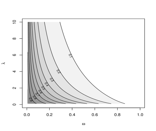
Figure 1: Kendall’s tau plotted as a function of $0\leq\omega\leq 1$ and $\lambda>0$ (curtailed at $\lambda=10$) for the BB9/PVF copula.

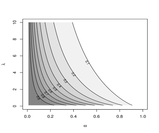
Figure 2: Spearman’s rho plotted as a function of $0\leq\omega\leq 1$ and $\lambda>0$ (curtailed at $\lambda=10$) for the BB9/PVF copula.

There is no such similar explicit form for Spearman’s rho for Archimedean copulas in general or the BB9/PVF copula in particular, but a numerically-derived graphical representation of it for BB9/PVF as a function of $\omega$ and $\lambda$ is also of interest; see Figure 2. The qualitative features of Figure 2 are very similar to those of Figure 1: $S$ too decreases from 1 (Fréchet copula) towards 0 (independence) as $\omega$ increases from 0 to 1 and from a positive value (Gumbel copula) towards 0 (independence) as $\lambda$ increases from 0 without bound. It is also suggested that $S\geq K$ for the BB9/PVF copula, but we have no proof. An upper bound for $S$ for the Gumbel copula, and hence for the BB9/PVF copula, is

$$S\leq\min\left[3\left\{\frac{2^{2(2-\omega)}}{(1+2^{1-\omega})^{2}}-1\right\},1\right].$$ (9)

The bound is non-trivial for $\omega>1+\log_{2}(\sqrt{3}-1)\simeq 0.55.$ See Appendix B for proof of this.

4. The bivariate APGW model

4.1 The model

We cannot simply replace the steps taken for the original PGW distribution for the adapted PGW distribution despite the existence of a parallel frailty result for APGW distributions in Result A1 in Appendix A: in Result A1, the TS distribution depends on $\kappa$, so the frailty distribution involved is not a single one to be shared by each failure time.

There is, however, a (still tractable) alternative which is to transform each marginal random variable, $T_{i}$, currently following an ordinary ${\rm PGW}(\gamma_{i},\tau_{i},\lambda)$ distribution to one, $Z_{i}$ say, following an ${\rm APGW}(\gamma_{i},\tau_{i},\lambda)$ distribution, using

$$Z_{i}=\left[(\tau+1)^{1-(1/\tau)}\left\{1+{\tau}(1+t^{\gamma})^{\tau}\right\}^{1/\tau}-(\tau+1)\right]^{1/\gamma},$$

$i=1,2.$ The resulting bivariate APGW distribution has survival function

$$S_{A}(z_{1},z_{2})=\exp\left[\lambda\left\{1-L_{A}^{\omega}(z_{1},z_{2})\right\}\right]$$ (10)

where

$$L_{A}(z_{1},z_{2}) = \left\{\frac{(\tau_{1}+1)}{\tau_{1}}\left(1+\frac{z_{1}^{\gamma_{1}}}{\tau_{1}+1}\right)^{\tau_{1}}-\frac{1}{\tau_{1}}\right\}^{1/\omega}$$ (11)

$$~{}~{}~{}~{}~{}~{}~{}~{}+\left\{\frac{(\tau_{2}+1)}{\tau_{2}}\left(1+\frac{z_{2}^{\gamma_{2}}}{\tau_{2}+1}\right)^{\tau_{2}}-\frac{1}{\tau_{2}}\right\}^{1/\omega}-1.$$

Of course, this is nothing other than introducing APGW marginals instead of PGW marginals into the BB9/PVF copula (8). (Survival function (10) is $\widehat{C}(S_{1,A}(z_{1}),S_{2,A}(z_{2}))$ where $S_{i,A}$ is the $i$th marginal APGW survival function, $i=1,2.$)

Special and limiting cases include bivariate Weibull ($(\tau_{1},\tau_{2})=(1,1)$), log-logistic/Burr Type XII ($(\tau_{1},\tau_{2})\to(0,0)$) and Gompertz distributions ($(\tau_{1},\tau_{2})$$\to(\infty,\infty)$). Their survival functions are all of the form (10) with $L_{A}$ functions given by

$$L_{A;W}(z_{1},z_{2})=(1+z_{1}^{\gamma_{1}})^{1/\omega}+(1+z_{2}^{\gamma_{2}})^{1/\omega}-1,$$

$$L_{A;B}(z_{1},z_{2})=\left\{1+\log(1+z_{1}^{\gamma_{1}})\right\}^{1/\omega}+\left\{1+\log(1+z_{2}^{\gamma_{2}})\right\}^{1/\omega}-1$$

and

$$L_{A;G}(z_{1},z_{2})=\exp(z_{1}^{\gamma_{1}}/\omega)+\exp(z_{2}^{\gamma_{2}}/\omega)-1,$$

respectively.

Because the bivariate APGW distribution of this section has the same copula as the bivariate PGW distribution of Section 2, all those aspects of dependence that are encapsulated in the copula, and explored in Section 3.4, apply to the bivariate APGW distribution in the same way as they do to the bivariate PGW distribution.

4.2 Conditional hazard functions and Clayton’s cross ratio dependence function

The investigations of Sections 3.2 and 3.3, which are not purely copula-dependent, need to be reworked for the bivariate APGW distribution. Because survival function $(\ref{SA})$ has the same form as survival function (1), the conditional hazard functions and Clayton’s cross ratio dependence function have the same form as before (3), (5) and (7), respectively, but with $L_{A}$ given by (11) replacing $L_{N}$ given by (2).

The claims made for the bivariate APGW distribution in the remainder of this section are based on formulae given in Appendix C. We find that for $h(z_{1}|Z_{2}\geq z_{2})$ we have:

$${\rm if}~{}~{}\gamma_{1}\geq 1~{}~{}{\rm and}~{}~{}\gamma_{1}\tau_{1}\geq 1~{}~{}{\rm then}~{}~{}h(z_{1}|Z_{2}\geq Z_{2})~{}~{}\textrm{is increasing},$$

corresponding to the $z_{2}=0$ case, and

$${\rm if}~{}~{}\gamma_{1}\leq 1~{}~{}{\rm and}~{}~{}\gamma_{1}\leq\frac{\omega}{1-\omega+\tau_{1}}~{}~{}{\rm then}~{}~{}h(z_{1}|Z_{2}\geq z_{2})~{}~{}\textrm{is decreasing},$$

which is a little more restricted than in the bivariate PGW case. And also, in the APGW case, we can only be sure that

$${\rm if}~{}~{}\gamma_{1}\leq 1~{}~{}{\rm and}~{}~{}\gamma_{1}\leq\frac{\omega}{1-\omega+\tau_{1}}~{}~{}{\rm then}~{}~{}h(x|Y=y)~{}~{}\textrm{is decreasing}$$

but, as in the bivariate PGW case, there is no simple guarantee of positivity.

As trailed above, the cross ratio dependence function is now

$$\theta_{A}(z_{1},z_{2})=1+\frac{1}{\lambda}\,\left(\frac{1}{\omega}-1\right)\,\frac{1}{\{L_{A}(z_{1},z_{2})\}^{\omega}}.$$

Its monotonicity properties — decreasingness in $\lambda$ and $\omega$ — remain as in the PGW case. The latter now follows by the same argument as in Section 3.3 except with $r_{i}=[(\tau_{i}+1)\{1+z_{i}^{\gamma_{1}}/(\tau_{i}+1)\}^{\tau_{i}}-1]/\tau_{i}$, $i=1,2.$

5. Application

The well-known retinopathy dataset of Huster, Brookmeyer, and Self (1989; henceforth HBS) (available in the survival package in R) consists of measurements of the time to blindness in each of their eyes for 197 individuals. For each individual, one eye was randomised to a laser treatment with the other eye acting as a control and, hence, survival times are naturally paired within individuals. The main focus of this study was to evaluate the effectiveness of the treatment, that is, to compare aspects of the marginal survival distributions (in the presence of dependence). However, a covariate indicating the diabetes type (juvenile or adult at age of onset) was also of interest.

We use the bivariate APGW distribution to analyse these data, first without the covariate (Section 5.1) and then with the addition of the covariate (Section 5.2). The ‘full’ bivariate APGW distribution that we consider is that of Section 4 with horizontal scale/AFT parameters added into each marginal, that is, the model with survival function $S_{A}(\phi_{1}z_{1},\phi_{2}z_{2})$ where $S_{A}$ is given by (10) and (11). This model has eight parameters:

$$(Z_{1},Z_{2})\sim\text{bivariate~{}APGW}(\underbrace{\lambda,\omega,}_{\text{dependence}}~{}\underbrace{\phi_{1},\gamma_{1},\tau_{1}}_{Z_{1}~{}\text{marginal}},~{}\underbrace{\phi_{2},\gamma_{2},\tau_{2}}_{Z_{2}~{}\text{marginal}}~{}).$$ (12)

However, for ease of optimisation in fitting models using maximum likelihood estimation, we will prefer to work in terms of the vector of unconstrained parameters, $\theta=(\theta_{\lambda},\theta_{\omega},\theta_{\phi_{1}},\theta_{\gamma_{1}},\theta_{\tau_{1}},\theta_{\phi_{2}},\theta_{\gamma_{2}},\theta_{\tau_{2}})^{T}$ where

$$\theta_{\lambda} = \log\lambda,\qquad\theta_{\omega}=\log\{\omega/(1-\omega)\},\qquad\theta_{\phi_{j}}=\log\phi_{j},$$

$$\theta_{\gamma_{j}} = \log\gamma_{j},\qquad\quad\theta_{\tau_{j}}=\log(\tau_{j}+1),$$

$j=1,2$. In the context of the retinopathy dataset, the index ‘1’ corresponds to treatment and the index ‘2’ to control.

5.1 Treatment effect (no covariate)

In this subsection, we consider a series of submodels of (12) investigating the treatment effect (without including the diabetes covariate). Table 1 compares the eight models arising from all combinations of the following constraints:

1. common scale $\phi_{1}=\phi_{2}=\phi$,

2. common power $\gamma_{1}=\gamma_{2}=\gamma$, and

3. common distribution $\tau_{1}=\tau_{2}=\tau$,

together with, as the first model, the unconstrained model. Each model has been fitted to the data using maximum likelihood, implemented using a Newton procedure via the standard nlm optimiser in R.

Table 1: Comparison of treatment models

Model	Common	dim$(\theta)$	$\ell(\theta)$	AIC	BIC	$\Delta_{\text{AIC}}$	$\Delta_{\text{BIC}}$	$K$
1	—	8	-824.24	1664.48	1690.74	2.36	8.93	0.24
2	$\phi$	7	-824.62	1663.25	1686.23	1.13	4.41	0.28
3	$\gamma$	7	-824.64	1663.28	1686.27	1.17	4.45	0.24
4	$\tau$	7	-824.71	1663.42	1686.40	1.30	4.59	0.18
5	$\phi,\gamma$	6	-826.45	1664.91	1684.61	2.79	2.79	0.18
6	$\phi,\tau$	6	-826.01	1664.02	1683.72	1.90	1.90	0.19
7	$\gamma,\tau$	6	-825.06	1662.12	1681.81	0.00	0.00	0.18
8	$\phi,\tau,\gamma$	5	-839.59	1689.19	1705.60	27.07	23.79	0.16

“Common” indicates which parameters (“pars”) are constrained to be equal,
$\ell(\theta)$ is the log-likelihood value, $\Delta_{\text{AIC}}=\text{AIC}-\min(\text{AIC})$, $\Delta_{\text{BIC}}=\text{BIC}-\min(\text{BIC})$,
$K$ is Kendall’s tau.

We see that both the AIC and BIC are considerably larger for Model 8 than for any of the other fitted models. Model 8 is the model with equal distributions for the treated and untreated groups; hence, there certainly appears to be a difference between these groups. On the other hand, the full flexibility of Model 1 with unconstrained parameters appears not to be required here. The model with both the lowest AIC and BIC is Model 7 which has common shape parameters, but different scales, that is, the basic distribution and shape of hazard is the same for these two treatment groups, but they have different scales; Figure 3 reveals that the fit to the data is excellent.

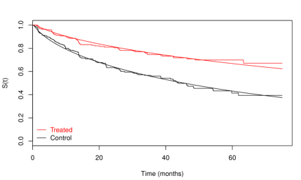
Figure 3: Kaplan–Meier (step) curves with model-based curves (smooth) overlaid for Model 7 of Table 1.

Table 2 displays parameter estimates for Model 7. As the two treatment groups here differ only with respect to their horizontal scale, we have the AFT property across groups. Thus, the quantile ratio is given by $\psi=\exp(\theta_{\phi_{2}}-\theta_{\phi_{1}})$ which is estimated as $\hat{\psi}=2.84$, that is, time to blindness is almost 3 times longer in eyes that receive laser treatment than in those that do not; the corresponding 95% confidence interval is $(1.64,4.92)$ (calculated using the delta method).

Table 2: Parameter estimates using Model 7

Parameter	$\theta_{\lambda}$	$\theta_{\omega}$	$\theta_{\gamma}$	$\theta_{\tau}$	$\theta_{\phi_{1}}$	$\theta_{\phi_{2}}$
Estimate	$-5.57$	1.52	1.52	0.14	$-0.07$	0.98
(S.E.)	(2.02)	(0.40)	(1.78)	(0.23)	(0.45)	(0.62)

Parameters shown are in unconstrained form, for example, $\theta_{\lambda}=\log\lambda$.
$\phi_{1}$ and $\phi_{2}$ are the scale parameters for the treatment and control group, respectively.

Note that all models fitted in Table 1 indicate quite a low level of correlation as measured by Kendall’s tau. In practice, however, it is often the case that the marginal models are fixed, for example, to Weibull or Gompertz distributions. In contrast, our more flexible APGW marginal distribution automatically selects the marginal models via the $\tau$ parameter(s); the estimated (common) $\tau$ value in our model is 0.15, with 95% confidence interval $(-0.26,0.78)$, which does not support Weibull or Gompertz margins ($\tau=1$, $\tau=\infty$). Misspecified marginal models have the potential to bias the measure of dependence. We briefly investigate the effect of the marginal model on Kendall’s tau by starting with Model 7 (of Table 2) and profiling over the $\tau$ parameter (including key models such as log-logistic, Weibull and Gompertz). The results are shown in Table 3 where we see that it is indeed the case that the value of $K$ varies with the choice of marginal model. In particular, the maximum likelihood marginal model with $\hat{\tau}=0.15$ yields a lower $K$ value than that of other $\tau$ values. Hence, fixing $\tau$ a priori has the potential to alter our view of the level of dependence. Interestingly, a 95% confidence interval for $K$ based on Model 7 is $(0.08,0.31)$. While this covers all $K$ values in Table 3 (just!), note from the Chi-squared statistics of Table 3 that higher $K$ values in models with Weibull or Gompertz margins are not supported by the data.

Table 3: Profiling $\tau$ for Model 7

Model	$\tau$	$K$	$\ell(\theta)$	$\chi^{2}_{1}$
Log-logistic	0.00	0.27	-826.89	3.66
	0.07	0.18	-825.24	0.36
Model 7	0.15	0.18	-825.06	0.00
	0.57	0.20	-826.74	3.36
Weibull	1.00	0.24	-829.03	7.94
	1.23	0.27	-829.45	8.78
	1.72	0.31	-829.60	9.09
Gompertz	$\infty$	0.31	-829.63	9.14

$\chi^{2}_{1}$ is the chi-squared statistic given by computing $2(\ell_{\text{Model 7}}-\ell_{\tau_{0}})$ where $\ell_{\text{Model 7}}$
is the likelihood for Model 7, and $\ell_{\tau_{0}}$ is the likelihood for $\tau$ fixed at $\tau_{0}$.

Note that the best-fitting treatment model of HBS is also one in which treatment enters the scale but not the shape. Their model comprises Weibull marginals together with a Clayton copula. It too has an AFT interpretation, their estimated quantile ratio turning out to be $2.62$, which is numerically similar to our result. The AIC and BIC values for HBS’s model are, respectively, 1667.21 and 1680.34, that is, the AIC value is much higher than that of our Model 7, while the BIC is slightly lower. The value of $K$ associated with HBS’s best-fitting model is 0.30, which, in light of Table 3, may be somewhat high. This could be a result of fixing to Weibull marginals or the use of a different (one-parameter) copula. Thus, while our proposed model can adapt readily to a variety of situations through its flexible copula and margins, the general use of simpler copula and marginal components will not work well in as many cases.

5.2 Diabetes effect (added covariate)

From the previous subsection, there is clearly a difference between treatment groups which manifests via a scale change rather than a shape change. It is also of interest to discover whether or not the type of diabetes – “juvenile” (the reference group here) or “adult” – is related to survival and, indeed, whether or not the diabetes effect interacts with the treatment effect. We will investigate this by extending the best treatment model from the previous section, Model 7, as follows:

$$\theta_{\gamma}=\theta_{\gamma,0}+\theta_{\gamma,1}D,\qquad\theta_{\phi_{1}}=\theta_{\phi_{1},0}+\theta_{\phi_{1},1}D,\qquad\theta_{\phi_{2}}=\theta_{\phi_{2},0}+\theta_{\phi_{2},1}D,$$

where $D$ is the binary diabetes indicator such that $D=1$ means that the diabetes type is adult. Note that, in line with our previous work, we are keeping the distributional parameter, $\tau$, as a covariate-independent parameter. Moreover, the copula parameters will also remain independent of the covariate for the moment.

The above model set-up permits a diabetes effect which interacts with treatment and, indeed, non-AFT effects via the inclusion of $D$ into the power shape parameter. We arrive at four models of interest characterized by combinations of:

1. $D$ has a non-AFT effect ($\theta_{\gamma,1}$ is free) or $D$ has an AFT effect ($\theta_{\gamma,1}=0$);

2. $D$ interacts with treatment ($\theta_{\phi_{1},1}$ and $\theta_{\phi_{2},1}$ are free) or not ($\theta_{\phi_{1},1}=\,{\color[rgb]{0,0,0}\theta_{\phi_{2},1}}\,=0$).

These four models were fitted to the data using maximum likelihood, and the results are summarised in Table 4. Model 7(b) has the lowest AIC and BIC values. Hence, it appears that diabetes interacts with treatment, and can be described by an AFT effect, that is, diabetes does not affect the shape of the distribution. This is in line with the diabetes model considered by HBS — although they did not investigate the potential shape effect of diabetes. We can see from Figure 4 that Model 7(b) provides an excellent fit to the data.

Table 4: Comparison of treatment models with diabetes covariate

Model	Diabetes Effect	$\dim(\theta)$	$\ell(\theta)$	AIC	BIC	$\Delta_{\text{AIC}}$	$\Delta_{\text{BIC}}$	$K$
7(a)	non-AFT int.	9	-820.86	1659.73	1689.28	0.38	3.67	0.19
7(b)	AFT int.	8	-821.67	1659.35	1685.61	0.00	0.00	0.19
7(c)	non-AFT	8	-822.74	1661.47	1687.74	2.13	2.13	0.17
7(d)	AFT	7	-825.04	1664.08	1687.06	4.73	1.45	0.18

“int.” is short for “interaction”, $\ell(\theta)$ is the log-likelihood value, $\Delta_{\text{AIC}}=\text{AIC}-\min(\text{AIC})$, $\Delta_{\text{BIC}}=\text{BIC}-\min(\text{BIC})$, $K$ is Kendall’s tau.

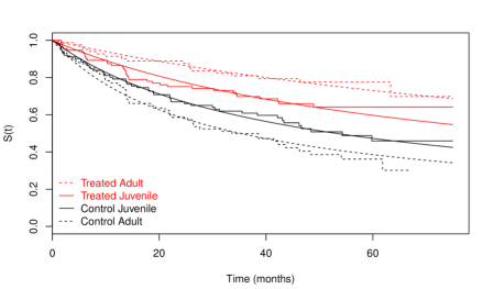
Figure 4: Kaplan–Meier (step) curves with model-based curves (smooth) overlayed for Model 7(b) of Table 4

Table 5: Parameter estimates using Model 7(b)

Parameter	$\theta_{\lambda}$	$\theta_{\omega}$	$\theta_{\gamma}$	$\theta_{\tau}$	$\theta_{\phi_{1},0}$	$\theta_{\phi_{1},1}$	$\theta_{\phi_{2},0}$	$\theta_{\phi_{2},1}$
Estimate	$-4.90$	1.40	0.99	0.22	$-0.05$	$-0.58$	0.55	0.42
(S.E.)	(0.96)	(0.37)	(0.58)	(0.11)	(0.52)	(0.35)	(0.55)	(0.28)

Parameters shown are in unconstrained form, for example, $\theta_{\lambda}=\log\lambda$.
$\phi_{1}$ and $\phi_{2}$ are the scale parameters for the treatment and control group, respectively.

An interesting finding is that, on the basis of BIC, the model without diabetes, the earlier Model 7, would be preferred to Model 7(b), whereas the improvement upon accounting for treatment was clear (compare Models 7 and 8). This reflects the fact that the difference between treatment groups is larger that the difference within treatment groups (via the diabetes type). On the other hand, based on the AIC and BIC, the models with a common diabetes effect would not be chosen over the treatment-only model (actually, Model 7(c) does have a very slightly lower AIC than Model 7 but this is not enough to warrant selection of the more complex Model 7(c)). In other words, a common diabetes effect is not plausible. This is clear from Figure 4 where the diabetes effect is reversed when comparing the treatment group to the control group. Furthermore, we see from Table 5 — which gives parameter estimates for Model 7(b) — that the diabetes effects within each group ($\theta_{\phi_{1},1}$ and $\theta_{\phi_{2},1}$, respectively) have different signs.

We can readily quantify the treatment effect for those with juvenile and adult diabetes in terms of quantile ratios. These are $\psi_{J}=\exp(\theta_{\phi_{2},0}-\theta_{\phi_{1},0})$ and $\psi_{A}=\exp\{(\theta_{\phi_{2},0}+\theta_{\phi_{2},1})-(\theta_{\phi_{1},0}+\theta_{\phi_{1},1})\}.$ Their estimates turn out to be $\hat{\psi}_{J}=1.81$, with 95% confidence interval $(1.12,2.91)$, and $\hat{\psi}_{A}=4.94$, with 95% confidence interval $(2.71,9.02)$, respectively. The conclusion is that time to blindness is almost doubled for treated individuals with juvenile diabetes, while the time to blindness is increased by a factor of almost five for treated individuals with adult diabetes. (Similar point estimates of quantile ratios arise from HBS’s model also.)

Finally, we also investigate whether or not covariate dependent copula parameters ($\lambda$ and $\omega$) might be needed. We therefore extended Model 7(b) (of Table 5) to have covariate dependent copula parameters. The resulting model (not shown) has AIC and BIC values of $1662.51$ and $1695.34$, respectively, which are both higher than those of Model 7(b). Moreover, the estimated $K$ values for $D=0$ and $D=1$ are respectively 0.19 and 0.20 which are numerically very close to each other — and indeed to that of Model 7(b). Furthermore, the fitted marginal models (not shown) are almost indistinguishable from those seen in Figure 4. Therefore, here, covariate-dependent copula parameters are not supported by the data, that is, Model 7(b) is sufficiently flexible. Of course, in other settings the level of correlation may vary with covariates, and modelling correlation on covariates in addition to the marginal distributions may avoid model misspecification (again noting the effect on Kendall’s tau of the marginal model as observed in Table 3).

6. Further remarks

In this article, we have proposed the novel combination of APGW marginal distributions and the BB9/PVF copula. We have shown that this specific unification is very natural and effective, yielding a new bivariate model whose marginals include many of the most popular survival distributions (and, indeed, whose marginals may differ in type via separate $\tau$ parameters, as shown in (12)). This flexibility, along with the variety of regression structures available, produces a very general overall modelling scheme which is useful in practice.

On the practical implementation of our model, it is worth highlighting that, based on the findings of BJN, we would not require a model with both $\lambda_{i}$ and $\phi_{i}$ (a vertical scale parameter and a horizontal scale parameter, respectively) appearing in the APGW marginal survival function $S_{i,A}(z_{i})$, $i=1,2$, simultaneously, due to their similar roles. However, here, with $\lambda_{1}=\lambda_{2}=\lambda$, where $\lambda$ also controls dependence within $\widehat{C}(u,v)$, we do not experience the issue. It is possible that estimation instability may arise within the model when $\phi_{1}=\phi_{2}=\phi$ particularly when $\omega$ is close to one as, in that case, $\lambda$ plays little role in characterising dependence and the margins then simply contain two scale parameters, $\lambda$ and $\phi$. Of course, one could contemplate models where $\lambda_{1}$ and $\lambda_{2}$ are unconstrained (that is, $\lambda_{1},\lambda_{2}\neq\lambda$) but, following BJN, we would then consider either $\text{APGW}(\lambda_{i},\phi_{i}=1,\gamma_{i},\tau_{i})$ or $\text{APGW}(\lambda_{i}=1,\phi_{i},\gamma_{i},\tau_{i})$ margins.

Shared frailty models like the ones of interest in this article are sometimes criticised on grounds of insufficient flexibility. A correlated frailty model is an attractive alternative, but in order to obtain one in the current context it is necessary to employ a defensible bivariate tempered stable/power variance distribution for the frailties. We are not aware of such a bivariate TS/PV model.

References

Bagdonaviçius, V. & Nikulin, M. (2002) Accelerated Life Model; Modeling and Statistical Analysis. Chapman & Hall/CRC.

Burke, K., Jones, M.C. & Noufaily, A. (2018) A flexible parametric modelling framework for survival analysis. Submitted.

Clayton, D.G. (1978) A model for association in bivariate life tables and its application in epidemiological studies of familial tendency in chronic disease incidence. Biometrika, 65, 141–151.

Crowder, M. (1989) A multivariate distribution with Weibull connections. J. Roy. Statist. Soc. Ser. B, 51, 93–107.

Dimitrakopoulou, T., Adamidis, K. & Loukas, S. (2007) A lifetime distribution with an upside-down bathtub-shaped hazard function. IEEE Trans. Reliab., 56, 308–311.

Duchateau, L. & Janssen, P. (2008) The Frailty Model. Springer.

Fischer, M. & Jakob, K. (2016) ptas distributions with application to risk management. J. Statist. Distributions Applic., 3, 1-18.

Gupta, P. & Gupta, R. (1996) Ageing characteristics of the Weibull mixtures. Prob. Eng. Info. Sci., 10, 591-600.

Hougaard, P. (1986) Survival models for heterogeneous populations derived from stable distributions. Biometrika, 73, 387-396.

Hougaard, P. (2000) Analysis of Multivariate Survival Data. Springer.

Huster, W.J., Brookmeyer, R. & Self, S.G. (1989) Modelling paired survival data with covariates. Biometrics, 45, 145–156.

Joe, H. (1997) Multivariate Models and Dependence Concepts. Chapman & Hall.

Joe, H. (2014) Dependence Modeling with Copulas. Chapman & Hall.

Jones, M.C. & Noufaily, A. (2015) Log-location-scale-log-concave distributions for survival and reliability analysis. Elec. J. Statist., 9, 2732–2750.

Nelsen, R.B. (2006) An Introduction to Copulas, 2nd. ed. Springer.

Nikulin, M. & Haghighi, F. (2009) On the power generalized Weibull family: model for cancer censored data. Metron, 67, 75–86.

Oakes, D. (1989) Bivariate survival models induced by frailties. J. Amer. Statist. Assoc., 84, 487–493.

Romeo, J.S., Meyer, R. & Gallardo, D.I. (2018) Bayesian bivariate survival analysis using the power variance function copula. Lifetime Data Anal., 24, 355–383.

Tweedie, M. (1984) An index which distinguishes between some important exponential families. In Ghosh, J. and Roy, J., editors, Statistics: Applications and New Directions, pp. 579–604.

Wienke, P. (2011) Frailty Models in Survival Analysis. Chapman & Hall.

Appendix A: Frailty Link for APGW Distribution

Write APGW$({\color[rgb]{0,0,0}\gamma,\,}\kappa,\lambda)$ for the adapted PGW distribution with proportionality parameter $\lambda>0$ and shape parameter $\kappa$ i.e. with c.h.f. $\lambda\,H_{A}(t^{\gamma};\kappa)$. Also, write the three-parameter version of the TS distribution as $TS(\omega,\xi,\theta)$, $0\leq\omega\leq 1$, $\xi>0,$ $\theta\geq 0$, having Laplace transform

$${\cal L}^{H}_{\omega,\xi,\theta}(s)=\exp\left[-\frac{\xi}{\omega}\left\{(\theta+s)^{\omega}-\theta^{\omega}\right\}\right]$$

and density $g^{H}_{\omega,\xi,\theta}$.

Result A1. Let $T|B=b\sim\textrm{APGW}({\color[rgb]{0,0,0}\gamma,\,}\kappa,b)$, $\kappa>0$, and let $B\sim$$\textrm{TS}\left(\omega,\frac{\kappa^{\omega-1}(\omega\kappa+1)}{(\kappa+1)^{\omega}},\frac{\kappa+1}{\kappa}\right)$. Then, $aT\sim\textrm{APGW}({\color[rgb]{0,0,0}\gamma,\,}\omega\kappa,1)$ where $a=$$\{(\kappa+1)/(\omega\kappa+1)\}^{1/\gamma}$.

Proof

$$S_{T}(t) = \int_{0}^{\infty}\exp\{-bH_{A}(t^{\gamma};\kappa)\}g^{H}_{\omega,\frac{\kappa^{\omega-1}(\omega\kappa+1)}{(\kappa+1)^{\omega}},\frac{\kappa+1}{\kappa}}(b)\,db$$

$$= {\cal L}^{H}_{\omega,\frac{\kappa^{\omega-1}(\omega\kappa+1)}{(\kappa+1)^{\omega}},\frac{\kappa+1}{\kappa}}\{H_{A}(t^{\gamma};\kappa)\}$$

$$= \exp\left[-\frac{\kappa^{\omega-1}(\omega\kappa+1)}{\omega(\kappa+1)^{\omega}}\right.$$

$$\left.~{}~{}~{}~{}~{}\times\left\{\left(\frac{\kappa+1}{\kappa}+\frac{\kappa+1}{\kappa}\left\{\left(1+\frac{t^{\gamma}}{\kappa+1}\right)^{\kappa}-1\right\}\right)^{\omega}-\left(\frac{\kappa+1}{\kappa}\right)^{\omega}\right\}\right]$$

$$= \exp\left[-\frac{(\omega\kappa+1)}{\omega\kappa}\left\{\left(1+\frac{t^{\gamma}}{\kappa+1}\right)^{\omega\kappa}-1\right\}\right]=\exp\left[-H_{A}\left\{\left(\frac{t}{a}\right)^{\gamma};\omega\kappa\right\}\right].\,\,\,\,\Box$$

Appendix B: Proof of (9)

For the Gumbel copula, $S=12\,{\cal I}-3$ where

$${\cal I} = \int_{0}^{1}\int_{0}^{1}\widehat{C}_{G}(u,v)\,dv\,du$$

$$= \int_{0}^{1}\int_{0}^{1}\exp\left[-\left\{(-\log u)^{1/\omega}+(-\log v)^{1/\omega}\right\}^{\omega}\right]\,dv\,du$$

$$= \int_{0}^{\infty}\int_{0}^{\infty}e^{-(x+y)}\exp\left\{-\left(x^{1/\omega}+y^{1/\omega}\right)^{\omega}\right\}\,dy\,dx$$

$$\leq \int_{0}^{\infty}\int_{0}^{\infty}\exp\left\{-(1+2^{\omega-1})(x+y)\right\}\,dy\,dx$$

$$= 1/(1+2^{\omega-1})^{2},$$

hence (9). Here, we have used the generalized mean inequality $(x^{1/\omega}+y^{1/\omega})^{\omega}\geq 2^{\omega-1}(x+y)$ for $0\leq\omega\leq 1$.

Appendix C: Formulae Underlying Claims in Section 4.2

From (11), we have

$$L_{A}^{10}(z_{1},z_{2})=\frac{\gamma_{1}}{\omega}z_{1}^{\gamma_{1}-1}\left(1+\frac{z_{1}^{\gamma_{1}}}{\tau_{1}+1}\right)^{\tau_{1}-1}\left\{\frac{(\tau_{1}+1)}{\tau_{1}}\left(1+\frac{z_{1}^{\gamma_{1}}}{\tau_{1}+1}\right)^{\tau_{1}}-\frac{1}{\tau_{1}}\right\}^{(1/\omega)-1}$$

and

$$L_{A}^{20}(z_{1},z_{2}) = \frac{\gamma_{1}}{\omega\,\tau_{1}}z_{1}^{\gamma_{1}-2}\left(1+\frac{z_{1}^{\gamma_{1}}}{\tau_{1}+1}\right)^{\tau_{1}-2}\left\{\frac{(\tau_{1}+1)}{\tau_{1}}\left(1+\frac{z_{1}^{\gamma_{1}}}{\tau_{1}+1}\right)^{\tau_{1}}-\frac{1}{\tau_{1}}\right\}^{(1/\omega)-2}$$

$$~{}~{}~{}~{}~{}~{}~{}~{}~{}~{}\times\left[\left\{(\gamma_{1}-1)(\tau_{1}+1)+\left(\frac{\gamma_{1}\,\tau_{1}}{\omega}-1\right)z_{1}^{\gamma_{1}}\right\}\left(1+\frac{z_{1}^{\gamma_{1}}}{\tau_{1}+1}\right)^{\tau_{1}}\right.$$

$$\left.~{}~{}~{}~{}~{}~{}~{}~{}~{}~{}~{}~{}~{}~{}~{}~{}~{}~{}~{}~{}~{}~{}~{}-\left\{\gamma_{1}-1+\frac{(\gamma_{1}\tau_{1}-1)}{\tau_{1}+1}z_{1}^{\gamma_{1}}\right\}\right].$$

Using these formulae in place of the equivalent formulae for $L_{N}$ in (4), we find that $h^{\prime}(z_{1}|Z_{2}\geq z_{2})$ is equal to positive terms times

$$\left[\left\{\frac{(\tau_{2}+1)}{\tau_{2}}\left(1+\frac{z_{2}^{\gamma_{2}}}{\tau_{2}+1}\right)^{\tau_{2}}-\frac{1}{\tau_{2}}\right\}^{1/\omega}-1\right]$$

$$~{}~{}~{}~{}~{}~{}~{}~{}~{}~{}\times\left[\left\{(\gamma_{1}-1)(\tau_{1}+1)+\left(\frac{\gamma_{1}\,\tau_{1}}{\omega}-1\right)z_{1}^{\gamma_{1}}\right\}\left(1+\frac{z_{1}^{\gamma_{1}}}{\tau_{1}+1}\right)^{\tau_{1}}\right.$$

$$\left.~{}~{}~{}~{}~{}~{}~{}~{}~{}~{}~{}~{}~{}~{}~{}~{}~{}~{}~{}~{}~{}~{}~{}-\left\{\gamma_{1}-1+\frac{(\gamma_{1}\tau_{1}-1)}{\tau_{1}+1}z_{1}^{\gamma_{1}}\right\}\right]$$ (13)

$$+\left\{\frac{(\tau_{1}+1)}{\tau_{1}}\left(1+\frac{z_{1}^{\gamma_{1}}}{\tau_{1}+1}\right)^{\tau_{1}}-\frac{1}{\tau_{1}}\right\}^{1/\omega}$$

$$~{}~{}~{}~{}~{}~{}~{}~{}~{}~{}\times\left[\left\{(\gamma_{1}-1)(\tau_{1}+1)+\left({\gamma_{1}\,\tau_{1}}-1\right)z_{1}^{\gamma_{1}}\right\}\left(1+\frac{z_{1}^{\gamma_{1}}}{\tau_{1}+1}\right)^{\tau_{1}}\right.$$

$$\left.~{}~{}~{}~{}~{}~{}~{}~{}~{}~{}~{}~{}~{}~{}~{}~{}~{}~{}~{}~{}~{}~{}~{}-\left\{\gamma_{1}-1+\frac{(\gamma_{1}\tau_{1}-1)}{\tau_{1}+1}z_{1}^{\gamma_{1}}\right\}\right]$$

from which the claims about the monotonicity properties of $h(z_{1}|Z_{2}\geq z_{2})$ in Section 4.2 follow. Similarly, the term in square brackets in the formula (6) when $L_{A}$ replaces $L_{N}$ is equal to positive terms times a formula identical to (13) except with the term ‘$\gamma_{1}\tau_{1}$’ replaced by zero in its fifth line. This sole difference is responsible for the conclusions in Section 4.2 concerning the monotonicity of $h(z_{1}|Z_{2}=z_{2})$.