First exit and Dirichlet problem for the nonisotropic tempered $\alpha$-stable processes

Abstract

This paper discusses the first exit and Dirichlet problems of the nonisotropic tempered $\alpha$-stable process $X_{t}$. The upper bounds of all moments of the first exit position $\left|X_{\tau_{D}}\right|$ and the first exit time $\tau_{D}$ are firstly obtained. It is found that the probability density function of $\left|X_{\tau_{D}}\right|$ or $\tau_{D}$ exponentially decays with the increase of $\left|X_{\tau_{D}}\right|$ or $\tau_{D}$, and $\mathrm{E}\left[\tau_{D}\right]\sim\left|\mathrm{E}\left[X_{\tau_{D}}\right]\right|$, $\mathrm{E}\left[\tau_{D}\right]\sim\mathrm{E}\left[\left|X_{\tau_{D}}-\mathrm{E}\left[X_{\tau_{D}}\right]\right|^{2}\right]$. Since $\mathrm{\Delta}^{\alpha/2,\lambda}_{m}$ is the infinitesimal generator of the anisotropic tempered stable process, we obtain the Feynman-Kac representation of the Dirichlet problem with the operator $\mathrm{\Delta}^{\alpha/2,\lambda}_{m}$. Therefore, averaging the generated trajectories of the stochastic process leads to the solution of the Dirichlet problem, which is also verified by numerical experiments.

1 Introduction

Lévy processes can effectively model the evolution processes with huge fluctuations, for example, fresh-water released by huge icebergs (Heinrich events), large fluctuations of the solar radiation steered by huge fluid outbursts on the surface of the sun. Sometimes, because of the particular bounded physical space, the extremely large oscillation should be suppressed and then the tempered Lévy processes are introduced 43 . While describing the diffusion in complex inhomogeneous media, the nonisotropic tempered $\alpha$-stable processes are natural and reasonable choice. These and the related processes have been studied more or less from different aspects in recent years. For example, according to the characteristic functions of stochastic processes, the corresponding Fokker-Planck equations are derived 1 ; 2 ; the numerical schemes are designed to solve the obtained Fokker-Planck equations 3 ; 4 ; the relationship between mean square displacement (MSD) of stochastic process and time is discussed 5 ; and there are also many discussions on the applications of the stochastic processes and the corresponding macroscopic equations 6 ; 7 ; 8 ; 9 .

The first hitting time is defined as the time when a certain condition is fulfilled by the random variable of interest for the first time 10 , which has a lot of potential applications. The example of first passage time naturally coming to our mind is the decision of an investor to buy or sell stock when its fluctuating prices reach a certain threshold 14 . Here, we focus on the time and position distribution of first exit from a sphere for the nonisotropic tempered $\alpha$-stable processes, and use the results to numerically solve the corresponding Dirichlet problem. The time and position distribution of first exit from a sphere are, respectively, defined as

$$\tau_{B(0,r)}=\inf\left\{t>0:\ X_{t}\notin B(0,r)\right\},\qquad\rho(x)=P\left[X_{\tau_{B(0,r)}}\in\mathrm{d}x,\,\tau_{B(0,r)}<\infty\right],$$

where $X_{t}\in\mathrm{R}^{d}$ is a stochastic process, and $X_{0}=x,\ \ x\in\mathrm{R}^{d}$; the notation $B(0,r)$ is a sphere centred at the origin and the radius is $r$; the random variable $\tau_{B(0,r)}$ is the first exit time and $\rho(x)$ is the probability density function (PDF) of the first exit position. For the isotropic stochastic processes, there are some results on first exit time and position distribution obtained by establishing equations. Letting $X_{0}=0$, when $X_{t}$ is the Brownian motion 10 ; 11 ; 12 ; 13 ,

$$\mathrm{E}\left[\tau_{B(0,r)}\right]=\frac{r^{2}}{2d},$$

and $\rho(x)$ is uniform distribution on the boundary of $B(0,r)$, and the trajectories of the process hit $\partial B(0,r)$ in finite time with probability 1, because of the continuity and isotropy of Brownian motion. When $X_{t}$ is the $\alpha$-stable Lévy process 14 ; 13 ; 15 ; 16 ; 17 ; 18 ; 19 ; 20 ; 21 ; 22 ; 23 ; 24 ; 25 ; 26 ; 27 ,

$$\mathrm{E}\left[\tau_{B(0,r)}\right]=\frac{\Gamma(d/2)r^{\alpha}}{2^{\alpha}\Gamma(1+\alpha/2)\Gamma(d/2+\alpha/2)};$$

due to the discontinuity of the paths of the processes, a particle starting at $X_{0}=0$, first escapes $B(0,r)$ and then lands in $B^{c}(0,r)$ (the complement of $B(0,r)$ in $\mathrm{R}^{d}$). Therefore, one needs to pay attention to the PDF $\rho(x)$ of the random variable $X_{\tau_{B(0,r)}}$ in $B^{c}(0,r)$. For $r<\infty$, $\rho(x)$ is given in 28 .

Although there are many achievements for Brownian motion and $\alpha$-stable processes, little research has been done on the average of first exit time and the distribution of random variable $X_{\tau_{B(0,r)}}$, when the process is nonisotropic tempered process. Part of the reason is that it is difficult to get effective results by establishing equations. Tempered stable laws wipe off the probability of extremely large jumps, so that all moments of the tempered stable process exist. Thus, this can be preferable in application where the moments have a physical meaning. And the diffusion of particles may be nonisotropic due to environmental effects. In many practical applications, the nonisotropic tempered model may be more reasonable for simulating real data; so this paper concentrates on its Dirichlet problem and connection to first exit problems. The Dirichlet problem of Brownian motion is

$$\mathrm{\Delta}u(x) =0,\qquad x\in D,$$ (1.1)

$$u(x) =g_{1}(x),\qquad x\in\partial D,$$

where $D$ is a domain in $\mathrm{R}^{d}$, $d\geq 2$, with sufficiently smooth boundary, and $g_{1}$ is a continuous function on the boundary. The Dirichlet problem of $\alpha$-stable Lévy process has the form

$$-(-\mathrm{\Delta})^{\alpha/2}u(x) =0,\qquad x\in D,$$ (1.2)

$$u(x) =g_{2}(x),\qquad x\in D^{c},$$

where $0<\alpha<2$, $g_{2}:\ D^{c}\to\mathrm{R}$ is a suitably regular function; and noting that $-(-\mathrm{\Delta})^{\alpha/2}$ is no longer a local operator, thus $\partial D$ is replaced by $D^{c}$ (the complement of $D$ in $\mathrm{R}^{d}$). Eq. (1.1) is a very classical model, and it has been sufficiently studied in almost every aspect. As for Eq. (1.2), it attracts the wide interests of researchers in recent years, e.g., the discussion of the numerical schemes and their implementations 29 ; 30 ; 31 ; 32 ; 33 ; the main challenge of numerically solving the equation comes from the nonlocality of the fractional Laplacian and the weak singularity of the solution of (1.2). The well-known Feynman-Kac representation 34 ; 35 implies that if $u(x)$ is a solution to Eq. (1.2), then

$$u(x)=\mathrm{E}_{x}\left[g_{2}\left(X_{\tau_{D}}\right)\right],\qquad x\in D,$$ (1.3)

where $\tau_{D}=\mathrm{inf}\left\{t>0:X_{t}\notin D\right\}$, and $X_{t}$ is the $\alpha$-stable Lévy process; for Eq. (1.1), the similar representation holds, just replacing $g_{2}$ by $g_{1}$ in Eq. (1.3) and taking $X_{t}$ to be Brownian motion. Eq. (1.3) suggests that the solution of Dirichlet problem Eq. (1.2) can be generated numerically by Monte Carlo algorithm 36 ; 37 ; 38 ; 39 ; 40 ; 41 . The advantage of Monte Carlo algorithm is that it can avoid the weak singularity and does not have the challenge of numerical cost for fractional Laplacian.

The Dirichlet problem for the asymmetric tempered fractional Laplacian, considered in this paper, is 42

$$\mathrm{\Delta}^{\alpha/2,\lambda}_{m}u(x) =f(x),\qquad x\in D,$$ (1.4)

$$u(x) =g(x),\qquad x\in D^{c},$$

where $\alpha\in(0,1)\cup(1,2)$, $f:\ D\to\mathrm{R}$ and $g:\ D^{c}\to\mathrm{R}$ are suitable functions; and

$$\mathrm{\Delta}^{\alpha/2,\lambda}_{m}u(x)= c_{m,\alpha}\int_{\mathrm{R}^{d}\setminus\{0\}}\left[u(x-y)-u(x)+\left(y\cdot\nabla_{x}u(x)\right)_{\chi_{\{|y|<1\}}}\right]\frac{m(y)}{\mathrm{e}^{\lambda|y|}|y|^{d+\alpha}}\mathrm{d}y$$ (1.5)

with $m(x)$ denoting the probability distribution of particles spreading in direction and $c_{m,\alpha}$ being a normalized constant. It seems that effectively solving Eq. (1.4) is not an easy task because of the nonsymmetry and nonlocal property of Eq. (1.5). We demonstrate that the operator $\mathrm{\Delta}^{\alpha/2,\lambda}_{m}$ is an infinitesimal generator of the nonisotropic tempered stable process and present the Feynman-Kac representation of Eq. (1.4). Then, the Monte Carlo algorithm may be a feasible approach.

This paper is organized as follows. In the next section, we introduce the characteristic functions and compound Poisson forms of anisotropic tempered stable processes. In section 3, we estimate all the moments of $\left|X_{\tau_{B(0,r)}}\right|$ and $\tau_{B(0,r)}$; and the relationship between $X_{\tau_{B(0,r)}}$ and $\tau_{B(0,r)}$ is given in the mean sense. In section 4, we obtain the Feynman-Kac representation of the Dirichlet problem for the anisotropic tempered fractional Laplacian $\mathrm{\Delta}^{\alpha/2,\lambda}_{m}$. The numerical experiments are performed in section 5. Finally, we conclude the paper with some discussions in section 6.

2 Tempered stable processes with Lévy symbol and notations

Let $X_{t}\,(t\geq 0)$ be the isotropic tempered stable process in $\mathrm{R}^{d}$. Then its characteristic function $\hat{p}(k,t)=\mathrm{E}\left[\mathrm{e}^{i(k\cdot X_{t})}\right]=\mathrm{e}^{t\psi(k)}$ 43 ; 44 , where the Lévy symbol

$$\psi(k)=\int_{\mathrm{R}^{d}\setminus\{0\}}\left(\mathrm{e}^{i(k\cdot x)}-1-i(k\cdot x)_{\chi\{|x|<1\}}\right)\nu(\mathrm{d}x)$$ (2.1)

and the Lévy measure

$$\nu(\mathrm{d}x)=c_{\alpha}\mathrm{e}^{-\lambda|x|}|x|^{-\alpha-d}$$

with $c_{\alpha}=\frac{\Gamma(d/2)}{2\pi^{d/2}|\Gamma(-\alpha)|}$, $0<\alpha<2$, and $\alpha\neq 1$. For the nonisotropic diffusion, the Lévy measure is given as

$$\nu(\mathrm{d}x)=c_{m,\alpha}\frac{m(x)}{\mathrm{e}^{\lambda|x|}|x|^{d+\alpha}}\mathrm{d}x;$$

to help understand the meaning of $m(x)$, one can notice that $\nu(\mathrm{d}x)$ has the polar coordinate form

$$c_{m,\alpha}\frac{m(\theta)}{\mathrm{e}^{\lambda r}r^{1+\alpha}}\mathrm{d}\theta\mathrm{d}r,$$

where $r\geq 0$, $\theta\in[0,2\pi)$ represents the direction, $m(\theta)$ is the probability distribution of particles in $\theta$-direction 42 , $c_{m,\alpha}$ is the normalized constant; and the anisotropic diffusion equation is

$$\frac{\partial p(x,t)}{\partial t}=\mathrm{\Delta}^{\alpha/2,\lambda}_{m}p(x,t).$$

The definitions of the two special cases of the tempered fractional Laplacian are given as 42

$Case\ I$: $0<\alpha<1$ or $m(y)$ is symmetric,

$$\mathrm{\Delta}^{\alpha/2,\lambda}_{m}p(x,t)=c_{m,\alpha}\int_{\mathrm{R}^{d}\setminus\{0\}}\left[p(x-y,t)-p(x,t)\right]\frac{m(y)}{\mathrm{e}^{\lambda|y|}|y|^{d+\alpha}}\mathrm{d}y$$ (2.2)

$Case\ II$: $1<\alpha<2$ and $m(y)$ is asymmetric,

$$\mathrm{\Delta}^{\alpha/2,\lambda}_{m}p(x,t)= c_{m,\alpha}\int_{\mathrm{R}^{d}\setminus\{0\}}\left[p(x-y,t)-p(x,t)+\left(y\cdot\nabla_{x}p(x,t)\right)_{\chi_{\{|y|<1\}}}\right]\frac{m(y)}{\mathrm{e}^{\lambda|y|}|y|^{d+\alpha}}\mathrm{d}y$$ (2.3)

$$-c_{m,\alpha}\Gamma(1-\alpha)\lambda^{\alpha-1}\left(\mathbf{b}\cdot\nabla_{x}p(x,t)\right),$$

where $\mathbf{b}=\int_{|\mathbf{\phi}|=1}\mathbf{\phi}m(\mathbf{\phi})\mathrm{d}\mathbf{\phi}$. From Eq. (2.2) and Eq. (2.3), we obtain the Lévy symbols of the corresponding anisotropic tempered stable processes,

$$\psi(k)=c_{m,\alpha}\int_{R^{d}\setminus\{0\}}\left(\mathrm{e}^{i(k\cdot y)}-1\right)\frac{m(y)}{\mathrm{e}^{\lambda|y|}|y|^{d+\alpha}}\mathrm{d}y$$ (2.4)

and

$$\psi(k)= c_{m,\alpha}\int_{R^{d}\setminus\{0\}}\left(\mathrm{e}^{i(k\cdot y)}-1-i(k\cdot y)_{\chi_{\{|y|<1\}}}\right)\frac{m(y)}{\mathrm{e}^{\lambda|y|}|y|^{d+\alpha}}\mathrm{d}y$$ (2.5)

$$+c_{m,\alpha}\Gamma(1-\alpha)\lambda^{\alpha-1}i\left(\mathbf{b}\cdot k\right),$$

which indicates that the anisotropic tempered stable process $X_{t}\,(t\geq 0)$ can be expressed by compound Poisson process. So, we have

$$X_{t}=\sum^{N(t)}_{i=0}Z_{i},\qquad 0<\alpha<1$$ (2.6)

and

$$X_{t}=\sum^{N(t)}_{i=0}Z_{i}-t\mathbf{\bar{b}},\qquad 1<\alpha<2,$$ (2.7)

where

$$\mathbf{\bar{b}}= -c_{m,\alpha}\int_{R^{d}\setminus\{0\}}y_{\chi\{|y|<1\}}\frac{m(y)}{\mathrm{e}^{\lambda|y|}|y|^{d+\alpha}}\mathrm{d}y$$ (2.8)

$$+c_{m,\alpha}\Gamma(1-\alpha)\lambda^{\alpha-1}\left(\mathbf{b}\right);$$

$Z_{0}$, $Z_{1}$, $Z_{2}$, $\cdots$, are a sequence of independent and identically distributed (i.i.d.) random variables taking valves in $\mathrm{R}^{d}$; the distribution of $Z_{i}$ is $\frac{m(x)\nu(\mathrm{d}x)}{\nu(|x|>0)}$; and $N(t)$ has a Poisson distribution

$$P\left(N(t)=n\right)=\mathrm{e}^{-\mu t}\frac{(\mu t)^{n}}{n!},$$

where $\mu=c_{m,\alpha}\nu(|x|>0)$ is renewal intensity. Let $\eta_{i}$ be the waiting time between the ($i-1$)-th and $i$-th jumps. Then

$$T[n]=\sum^{n}_{i=1}\eta_{i},$$

which leads to $N(t)=\max\{n\geq 0:\ T[n]\leq t\}$.

Since the stable process is a compound Poisson process, naturally we can consider all the moments of $\tau_{B(0,r)}$ and $\left|X_{\tau_{B(0,r)}}\right|$ based on the compound Poisson processes.

3 First exit position and time

The average first exit time 45 is a useful observation; here we provide the estimate of it for the processes discussed in the paper. Define

$$M_{N(t)}=\max_{0\leq s\leq t}|X_{s}|.$$

Theorem 1

Let $D$ be a bounded domain in $\mathrm{R}^{d}$ and $X_{t}$ the stochastic process $\mathrm{Eq}$. (2.6) or $\mathrm{Eq}$. (2.7), $D\subseteq B(x,r)$. If $P(|Z|>2r)>0$, then

$$\mathrm{E}\left[\tau_{D}\right]\leq\frac{1}{\mu P(|Z|>2r)}.$$

Proof

Since $D$ is a bounded domain, there exists a sphere $B(x,r),\ 0<r<\infty$ such that $D$ is its subset. Thus, we have

$$P\left(\tau_{D}\leq\tau_{B(x,r)}\right)=1.$$ (3.1)

For $0<\alpha<1$, computing probabilities by conditioning, we have

$$P\left(M_{N(t)}\leq r\right)=\sum^{\infty}_{n=0}P\left(M_{n}\leq r\right)\mathrm{e}^{-\mu t}\frac{(\mu t)^{n}}{n!}.$$

Since

$$P\left(M_{n}\leq r\right)\leq P\left(\max_{0\leq i\leq n}|Z_{i}|\leq 2r\right)=\left(P(|Z|\leq 2r)\right)^{n},$$

there exists

$$P\left(M_{N(t)}\leq r\right)\leq\mathrm{e}^{-\mu tP(|Z|>2r)}.$$ (3.2)

Noting that $P\left({\tau_{B(0,r)}>t}\right)=P\left(M_{N(t)}\leq r\right)$, Eq. (3.2) implies

$$\mathrm{E}\left[\tau_{B(0,r)}\right] =\int^{\infty}_{0}P\left({\tau_{B(0,r)}>t}\right)\mathrm{d}t$$

$$=\int^{\infty}_{0}P\left(M_{N(t)}\leq r\right)\mathrm{d}t$$

$$\leq\int^{\infty}_{0}\mathrm{e}^{-\mu tP(|Z|>2r)}\mathrm{d}t$$

$$=\frac{1}{\mu P(|Z|>2r)}.$$

Similarly, when $1<\alpha<2$, we also have

$$P\left(M_{N(t)}\leq r\right)\leq P\left(\max_{0\leq i\leq N(t)}|Z_{i}|\leq 2r\right)=\mathrm{e}^{-\mu tP(|Z|>2r)},$$

which means

$$\mathrm{E}\left[\tau_{B(0,r)}\right]\leq\frac{1}{\mu P(|Z|>2r)}.$$

Combining above and Eq. (3.1) leads to

$$\mathrm{E}\left[\tau_{D}\right]\leq\mathrm{E}\left[\tau_{B(0,r)}\right]\leq\frac{1}{\mu P(|Z|>2r)}.$$

Corollary 2

If $C<\mu P(|Z|>2r)$, we have

$$\mathrm{E}\left[\mathrm{e}^{C\tau_{B(0,r)}}\right]\leq\frac{C}{\mu P(|Z|>2r)-C}+1.$$ (3.3)

Proof

The proof of Theorem 1 shows that

$$\int^{\infty}_{0}\mathrm{e}^{Ct}P\left({\tau_{B(0,r)}>t}\right)\mathrm{d}t =\int^{\infty}_{0}\mathrm{e}^{Ct}P\left(M_{N(t)}\leq r\right)$$ (3.4)

$$\leq\int^{\infty}_{0}\mathrm{e}^{Ct}\mathrm{e}^{-\mu tP(|Z|>2r)}\mathrm{d}t$$

$$=\frac{1}{\mu P(|Z|>2r)-C}.$$

Let $f(t)$ be the PDF of $\tau_{B(0,r)}$. Making integration by parts leads to

$$\int^{\infty}_{0}\mathrm{e}^{Ct}P\left({\tau_{B(0,r)}>t}\right)\mathrm{d}t =-\frac{1}{C}+\frac{1}{C}\int^{\infty}_{0}\mathrm{e}^{Ct}f(t)\mathrm{d}t$$

$$=-\frac{1}{C}+\frac{1}{C}\mathrm{E}\left[\mathrm{e}^{C\tau_{B(0,r)}}\right]\leq\frac{1}{\mu P(|Z|>2r)-C},$$

which results in

$$\mathrm{E}\left[\mathrm{e}^{C\tau_{B(0,r)}}\right]\leq\frac{C}{\mu P(|Z|>2r)-C}+1.$$

Remark 3.1

If $D$ is a bounded domain and $P(|Z|>2r)>0$, then all the moments of the first exit time of compound Poisson processes are finite. The PDF of $\tau_{B(0,r)}$ decays exponentially when $t$ is large enough. The power of exponential decay becomes smaller for bigger $\alpha$ when $\alpha>1$; refer to Fig. 1 (for the details of simulation, see appendix).

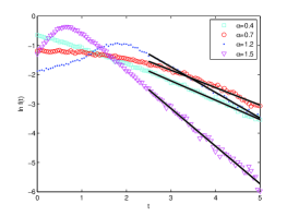
Fig. 1: PDF of $\tau_{B(0,1)}$ with $\lambda=0.01$ and $d=2$ for $\alpha=0.4$ (turquoise square), $\alpha=0.7$ (red circle), $\alpha=1.2$ (blue point), and $\alpha=1.5$ (magenta triangle). The parameters are: sample number $n=1.5\times 10^{5}$, $X_{0}=[0,\ 0]$, $\Delta t=5\times 10^{-4}$, $b=10$, $m(\theta)=1/{4\pi}$ for $\arg(\theta)\in(0,\ \pi)$ and $m(\theta)=3/{4\pi}$ for $\arg(\theta)\in(\pi,\ 2\pi)$.

Another useful observation is the first exit position 46 . According to the compound Poisson processes, we estimate $\mathrm{E}\left[\left|X_{\tau_{B(0,r)}}\right|\right]$, where $\mathrm{E}$ denotes the average over space and time when the r.v. is $X_{\tau_{B(0,r)}}$.

Proposition 3

Let $r>0$, $\xi>0$, $X_{t}=\sum^{N(t)}_{i=0}Z_{i}$ be compound Poisson process and $Z,\,Z_{1},\,Z_{2},\cdots$ be i.i.d.. Then

$$P\left(|Z|>2r+\xi\right)G(\mu)\leq P\left(\left|X_{\tau_{B(0,r)}}\right|-r>\xi\right)\leq P\left(|Z|>\xi\right)G(\mu),$$

where $G(\mu)=\int^{\infty}_{0}\left(1-\mathrm{e}^{-\mu t}\right)f(t)\mathrm{d}t$, and $f(t)$ is the PDF of $\tau_{B(0,r)}$.

Proof

$P\left(\left|X_{T_{B(0,r)}}\right|-r>\xi\right)$

$$=\int^{\infty}_{0}P\left(\left|X_{t}\right|>r+\xi\right)f(t)\mathrm{d}t$$

$$=\int^{\infty}_{0}\sum^{\infty}_{n=1}P\left(\left|\sum^{n}_{i=0}Z_{i}\right|>r+\xi\right)\mathrm{e}^{-\mu t}\frac{(\mu t)^{n}}{n!}f(t)\mathrm{d}t$$

$$=\int^{\infty}_{0}\sum^{\infty}_{n=1}\int_{|x|\leq r}P\left(\left|Z_{n}+x\right|>r+\xi\right)P\left(M_{n-1}\leq r,\ \sum^{n-1}_{i=0}Z_{i}\in\mathrm{d}x\right)\mathrm{e}^{-\mu t}\frac{(\mu t)^{n}}{n!}f(t)\mathrm{d}t.$$

On the other hand, for $|x|\leq r$, we have

$$P\left(\left|Z\right|>2r+\xi\right)\leq P\left(\left|Z_{n}+x\right|>r+\xi\right)\leq P\left(\left|Z\right|>\xi\right).$$ (3.5)

Then

$$P\left(\left|X_{T_{B(0,r)}}\right|-r>\xi\right)\leq P\left(|Z|>\xi\right)\int^{\infty}_{0}\left(1-\mathrm{e}^{-\mu t}\right)f(t)\mathrm{d}t$$

and

$$P\left(\left|X_{T_{B(0,r)}}\right|-r>\xi\right)\geq P\left(|Z|>2r+\xi\right)\int^{\infty}_{0}\left(1-\mathrm{e}^{-\mu t}\right)f(t)\mathrm{d}t.$$

The proof is completed.

By Proposition 3, for $\xi>1$, there exists

$$P\left(|Z|>r(1+\xi)\right)G(\mu)\leq P\left(\frac{\left|X_{\tau_{B(0,r)}}\right|}{r}>\xi\right)\leq P\left(|Z|>r(\xi-1)\right)G(\mu).$$ (3.6)

While for $X_{t}=\sum^{N(t)}_{i=0}Z_{i}-t\mathbf{\bar{b}}$, the estimate of $P\left(\left|X_{\tau_{B(0,r)}}\right|-r>\xi\right)$ is slightly different. Because there are two ways to escape from the sphere $B(0,r)$, i.e., the escape is due to the shifted term $t\mathbf{\bar{b}}$ or the jump $Z_{N(t)}$. Let $J^{c}$ and $J$ represent two escape modes, respectively.

Define

$$J^{c}=\{T\left[N(\tau_{B(0,r)})\right]<\tau_{B(0,r)}\},\qquad J=\{T\left[N(\tau_{B(0,r)})\right]=\tau_{B(0,r)}\}.$$

Corollary 4

For $r>0$, $\xi>0$, $X_{t}=\sum^{N(t)}_{i=0}Z_{i}-t\mathbf{\bar{b}}$, we have

$$P\left(\left|X_{\tau_{B(0,r)}}\right|-r>\xi\right)\leq P\left(|Z|>\xi\right)G(\mu).$$

Proof

Because of the continuity of the shifted term $t\mathbf{\bar{b}}$, we have

$$P\left(\left|X_{\tau_{B(0,r)}}\right|-r>\xi\right) =P\left(\left|X_{\tau_{B(0,r)}}\right|-r>\xi,J\right)+P\left(\left|X_{\tau_{B(0,r)}}\right|-r>\xi,J^{c}\right)$$

$$=P\left(\left|X_{\tau_{B(0,r)}}\right|-r>\xi,J\right),$$

which implies that

$P\left(\left|X_{\tau_{B(0,r)}}\right|-r>\xi\right)$

$$=\int^{\infty}_{0}\sum^{\infty}_{n=1}P\left(\left|\sum^{n}_{i=0}Z_{i}-t\mathbf{\bar{b}}\right|>r+\xi,J\right)\mathrm{e}^{-\mu t}\frac{(\mu t)^{n}}{n!}f(t)\mathrm{d}t$$

$$=\int^{\infty}_{0}\sum^{\infty}_{n=1}\int_{|x|\leq r}P\left(\left|Z_{n}+x\right|>r+\xi,J\right)P\left(\max_{0\leq s<t}|X_{s}|\leq r,\ \sum^{n-1}_{i=0}Z_{i}-t\mathbf{\bar{b}}\in\mathrm{d}x\right)\mathrm{e}^{-\mu t}\frac{(\mu t)^{n}}{n!}f(t)\mathrm{d}t.$$

For $|x|\leq r$,

$$P\left(\left|Z_{n}+x\right|>r+\xi,J\right)\leq P\left(\left|Z_{n}+x\right|>r+\xi\right)\leq P\left(\left|Z\right|>\xi\right).$$ (3.7)

Then, we have

$$P\left(\left|X_{\tau_{B(0,r)}}\right|-r>\xi\right)\leq P\left(|Z|>\xi\right)\int^{\infty}_{0}\left(1-\mathrm{e}^{-\mu t}\right)f(t)\mathrm{d}t.$$

The proof is completed.

By Corollary 4, for $\xi>1$, there exists

$$P\left(\frac{\left|X_{\tau_{B(0,r)}}\right|}{r}>\xi\right)\leq P\left(|Z|>r(\xi-1)\right)G(\mu).$$ (3.8)

These two results Eq. (3.6) and Eq. (3.8) lead to the estimates of the moments of $\left|X_{\tau_{B(0,r)}}\right|$.

Theorem 5

Let $0<q<\infty$, $0<r<\infty$, and $X_{t}$ be the stochastic process $\mathrm{Eq}$. (2.6) or $\mathrm{Eq}$. (2.7). If $\mathrm{E}\left[|Z|^{q}\right]<\infty$, then

$$\mathrm{E}\left[\left|X_{\tau_{B(0,r)}}\right|^{q}\right]<\infty.$$

Proof

For $X_{t}=\sum^{N(t)}_{i=0}Z_{i}$, by Eq. (3.6), we have

$$\frac{\mathrm{E}\left[\left|X_{\tau_{B(0,r)}}\right|^{q}\right]}{r^{q}} =\int^{\infty}_{0}q\xi^{q-1}P\left(\frac{\left|X_{\tau_{B(0,r)}}\right|}{r}>\xi\right)\mathrm{d}\xi$$

$$\leq 2^{q}+q\int^{\infty}_{2}\xi^{q-1}P\left(\frac{\left|X_{\tau_{B(0,r)}}\right|}{r}>\xi\right)\mathrm{d}\xi$$

$$\leq 2^{q}+G(\mu)q\int^{\infty}_{2}\xi^{q-1}P\left(\frac{|Z|}{r}>\frac{\xi}{2}\right)\mathrm{d}\xi$$

$$=2^{q}+G(\mu)q(2/r)^{q}\int^{\infty}_{r}\xi^{q-1}P\left(|Z|>\xi\right)\mathrm{d}\xi.$$

The proof is completed.

At the same time, the lower bound of the estimate can also be obtained as

$$\frac{\mathrm{E}\left[\left|X_{\tau_{B(0,r)}}\right|^{q}\right]}{r^{q}} \geq\int^{\infty}_{1}q\xi^{q-1}P\left(\frac{\left|X_{\tau_{B(0,r)}}\right|}{r}>\xi\right)\mathrm{d}\xi$$

$$\geq G(\mu)q\int^{\infty}_{1}\xi^{q-1}P\left(\frac{|Z|}{r}>2\xi\right)\mathrm{d}\xi$$

$$=G(\mu)q(2r)^{-q}\int^{\infty}_{2r}\xi^{q-1}P\left(|Z|>\xi\right)\mathrm{d}\xi.$$

Similarly, for $X_{t}=\sum^{N(t)}_{i=0}Z_{i}-t\mathbf{\bar{b}}$, by Eq. (3.8), there exists

$$\frac{\mathrm{E}\left[\left|X_{\tau_{B(0,r)}}\right|^{q}\right]}{r^{q}}\leq 2^{q}+G(\mu)q(2/r)^{q}\int^{\infty}_{r}\xi^{q-1}P\left(|Z|>\xi\right)\mathrm{d}\xi.$$

Theorem 5 shows that $\mathrm{E}\left[\left|X_{\tau_{B(0,r)}}\right|^{q}\right]<\infty$ for the tempered stable process $X_{t}$.

Corollary 6

For the tempered stable process $X_{t}$, if $\beta\leq\lambda$, then

$$\mathrm{E}\left[\exp\left(\beta\left|X_{\tau_{B(0,r)}}\right|\right)\right]<\infty.$$

Proof

For $0<\alpha<1$, according to Proposition 3, there exists

$$\mathrm{E}\left[\exp\left(\beta\left|X_{\tau_{B(0,r)}}\right|\right)\right]$$

$$=\mathrm{e}^{\beta r}+\int^{\infty}_{r}\beta\mathrm{e}^{\beta\xi}P\left(\left|X_{\tau_{B(0,r)}}\right|>\xi\right)\mathrm{d}\xi$$

$$=\mathrm{e}^{\beta r}+\int^{\infty}_{0}\beta\mathrm{e}^{\beta(\xi_{0}+r)}P\left(\left|X_{\tau_{B(0,r)}}\right|-r>\xi_{0}\right)\mathrm{d}\xi_{0}$$

$$\leq\mathrm{e}^{\beta r}+\int^{\infty}_{0}\beta\mathrm{e}^{\beta(\xi_{0}+r)}P\left(\left|Z\right|>\xi_{0}\right)\mathrm{d}\xi_{0}$$

$$=\frac{c_{m,\alpha}\mathrm{e}^{\beta r}}{{\nu(|Z|>0)}}\int^{\infty}_{0}\mathrm{e}^{(\beta-\lambda)\xi_{0}}\xi_{0}^{-1-\alpha}\mathrm{d}\xi_{0}.$$

As $1<\alpha<2$, Corollary 4 implies

$$\mathrm{E}\left[\exp\left(\beta\left|X_{\tau_{B(0,r)}}\right|\right)\right]$$

$$\leq\frac{c_{m,\alpha}\mathrm{e}^{\beta r}}{{\nu(|Z|>0)}}\int^{\infty}_{0}\mathrm{e}^{(\beta-\lambda)\xi_{0}}\xi_{0}^{-1-\alpha}\mathrm{d}\xi_{0}.$$

Corollary 6 also shows that the PDF $p(x)$ of $\left|X_{\tau_{B(0,r)}}\right|$ decays exponentially, as $\left|X_{\tau_{B(0,r)}}\right|$ becomes large, confirmed by Fig. 2.

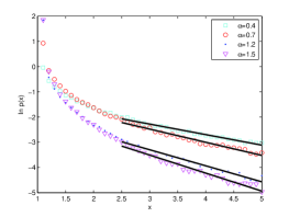
Fig. 2: Simulation of PDF of $\left|X_{\tau_{B(0,1)}}\right|$ with $\lambda=0.01$ and $d=2$ for $\alpha=0.4$ (turquoise square), $\alpha=0.7$ (red circle), $\alpha=1.2$ (blue point), and $\alpha=1.5$ (magenta triangle). The other parameters are the same as those in Fig. 1.

Generally, the moments of the tempered stable process $X_{t}$ are closely related to $t$. So is there a similar relationship between $\left|X_{\tau_{D}}\right|$ and $\tau_{D}$? Firstly, let’s discuss the symmetric tempered stable process; the following proposition demonstrates that the second moment of the process $|X_{t}|$ linearly increases with $t$.

Proposition 7

If $X_{t}$ is the symmetric tempered stable process and $X_{0}=0$, then the second moment of it is independent of the dimension $d$, and there is

$$\mathrm{E}\left[\left|X_{t}\right|^{2}\right]=\alpha|1-\alpha|\lambda^{\alpha-2}t.$$

Proof

$$\mathrm{E}\left[\left|X_{t}\right|^{2}\right] =\sum^{\infty}_{n=0}\mathrm{E}\left[\left|\sum^{N(t)}_{i=0}Z_{i}\right|^{2}\bigg{|}N(t)=n\right]P\left[N(t)=n\right]$$ (3.9)

$$=\sum^{\infty}_{n=0}\mathrm{E}\left[\left|\sum^{n}_{i=0}Z_{i}\right|^{2}\right]P\left[N(t)=n\right].$$

The i.i.d. property and symmetry of $\nu(\mathrm{d}x)$ lead to

$$\mathrm{E}\left[\left|X_{t}\right|^{2}\right] =\mathrm{E}[|Z|^{2}]\sum^{\infty}_{n=0}n\mathrm{e}^{-\mu t}\frac{(\mu t)^{n}}{n!}$$ (3.10)

$$=\frac{\alpha|1-\alpha|\lambda^{\alpha-2}}{\nu(|x|>0)}\mu t$$

$$=\alpha|1-\alpha|\lambda^{\alpha-2}t,$$

which completes the proof.

For the symmetric tempered stable process, $\mathrm{E}\left[|X_{t}|^{2}\right]\sim t$. Can we also expect $\mathrm{E}\left[\left|X_{\tau_{B(0,r)}}\right|^{2}\right]\sim\mathrm{E}\left[\tau_{B(0,r)}\right]$ 47 ? See the following theorem.

Theorem 8

Assume that the symmetric stochastic process $X_{t}$ has the stationary and independent increments, and

$$\mathrm{E}\left[|X_{t}|^{2}\right]=Ct,$$

where $C$ is a constant; $D$ is a bounded domain, and $\mathrm{E}\left[\tau_{D}\right]<\infty$. Then

$$\mathrm{E}\left[\left|X_{\tau_{D}}\right|^{2}\right]=C\cdot\mathrm{E}\left[\tau_{D}\right].$$

Proof

Let $\tau(n_{0})=\min\{\tau_{D},n_{0}\}$, which is a finite stopping time. Since the increments are stationary and independent, there is

$$\mathrm{E}\left[\left|X_{\tau(n_{0})}\right|^{2}\right] =\lim_{n\to\infty}\mathrm{E}\left[\left|X\left(\frac{1}{n}\right)\mathbf{1}_{\left\{\tau(n_{0})\geq\frac{1}{n}\right\}}+X\left(\frac{2}{n}-\frac{1}{n}\right)\mathbf{1}_{\left\{\tau(n_{0})\geq\frac{2}{n}\right\}}+\cdots\right|^{2}\right]$$

$$=\lim_{n\to\infty}\mathrm{E}\left[\left|X\left(\frac{1}{n}\right)\right|^{2}\right]\sum^{n_{0}n}_{i=1}P\left(\tau(n_{0})\geq\frac{i}{n}\right)$$

$$=C\lim_{n\to\infty}\frac{1}{n}\sum^{n_{0}n}_{i=1}P\left(\tau(n_{0})\geq\frac{i}{n}\right)$$

$$=C\int^{n_{0}}_{0}P\left(\tau(n_{0})\geq t\right)\mathrm{d}t.$$

The fact

$$\lim_{n_{0}\to\infty}\tau(n_{0})=\tau_{D},$$

leads to

$$\lim_{n_{0}\to\infty}\mathrm{E}\left[\left|X_{\tau(n_{0})}\right|^{2}\right]=\mathrm{E}\left[\left|X_{\tau_{D}}\right|^{2}\right]=C\mathrm{E}\left[\tau_{D}\right],$$ (3.11)

which completes the proof.

According to Theorem 8, one can get $\mathrm{E}\left[\tau_{B(0,r)}\right]$ of the symmetric Brownian motion. Since

$$\mathrm{E}\left[\left|X_{t}\right|^{2}\right]=2dt,$$

which leads to

$$\mathrm{E}\left[\tau_{B(0,r)}\right]=\mathrm{E}\left[\left|X_{\tau_{B(0,r)}}\right|^{2}\right]/{2d}=r^{2}/{2d}.$$

There’s another way to prove Theorem 8. Let

$$M_{t}=\left|X_{t}\right|^{2}-Ct.$$

Define the natural filtration of the process $X_{t}$ as

$$\mathcal{G}^{X}_{t}=\sigma\left\{X_{s}:\ 0\leq s\leq t\right\}.$$

Then, we have

$$\mathrm{E}\left[M_{t}|\mathcal{G}^{X}_{s}\right] =\mathrm{E}\left[\left|X_{t}-X_{s}\right|^{2}|\mathcal{G}^{X}_{s}\right]-Ct+\left|X_{s}\right|^{2}\qquad(s\leq t)$$

$$=\left|X_{s}\right|^{2}-Cs$$

$$=M_{s},$$

showing that $M_{t}$ is a martingale. Thus, using Doob’s optional stopping theorem leads to

$$\mathrm{E}\left[M_{\tau_{D}}\right]=\mathrm{E}\left[M_{0}\right]=0,$$

which implies that Theorem 8 holds.

For the anisotropic tempered stable process $X_{t}$, we calculate its second moment. In the two dimensional case, define

$$Z_{i}=(r_{i}\cos\theta_{i},r_{i}\sin\theta_{i}),$$

where the PDF of $r_{i}$ is

$$\frac{\mathrm{e}^{-\lambda r}r^{-1-\alpha}}{\int^{\infty}_{0}\mathrm{e}^{-\lambda r}r^{-1-\alpha}\mathrm{d}r},$$ (3.12)

and the PDF of $\theta_{i}$ is $m(\theta)$, defined on $[0,2\pi]$. Note that $r_{i}$($\theta_{i}$) is i.i.d. random variable, and $r_{i}$ and $\theta_{i}$ are independent of each other. When $0<\alpha<1$ in (3.12), for Eq. (2.6), there exists

$$\mathrm{E}\left[|X_{t}|^{2}\right] =\sum^{\infty}_{n=0}\mathrm{E}\left[\left|\sum^{n}_{i=0}Z_{i}\right|^{2}\right]P\left[N(t)=n\right]$$ (3.13)

$$=\sum^{\infty}_{n=0}\mathrm{E}\left[\left(\sum^{n}_{i=0}r_{i}\cos\theta_{i}\right)^{2}+\left(\sum^{n}_{i=0}r_{i}\sin\theta_{i}\right)^{2}\right]P\left[N(t)=n\right]$$

$$=\sum^{\infty}_{n=0}\left(n\mathrm{E}\left[r^{2}_{1}\right]+n(n-1)\left(\mathrm{E}\left[r_{1}\right]\right)^{2}\left[\left(\mathrm{E}\left[\cos\theta_{1}\right]\right)^{2}+\left(\mathrm{E}\left[\sin\theta_{1}\right]\right)^{2}\right]\right)P\left[N(t)=n\right]$$

$$=\mathrm{E}\left[r^{2}_{1}\right]\mu t+\left(\mathrm{E}\left[r_{1}\cos\theta_{1}\right]\right)^{2}(\mu t)^{2}+\left(\mathrm{E}\left[r_{1}\sin\theta_{1}\right]\right)^{2}(\mu t)^{2}.$$

The MSD of $X_{t}$ is a linear function of $t$:

$$\mathrm{E}\left[\left|X_{t}-\mathrm{E}[X_{t}]\right|^{2}\right]$$ (3.14)

$$=\sum^{\infty}_{n=0}\mathrm{E}\left[\left|\sum^{n}_{i=0}Z_{i}-\mathrm{E}\left[\sum^{n}_{i=0}Z_{i}\right]\right|^{2}\right]P\left[N(t)=n\right]$$

$$=\sum^{\infty}_{n=0}\mathrm{E}\left[\left(\sum^{n}_{i=0}\left(r_{i}\cos\theta_{i}-\mathrm{E}[r_{i}\cos\theta_{i}]\right)\right)^{2}+\left(\sum^{n}_{i=0}\left(r_{i}\sin\theta_{i}-\mathrm{E}[r_{i}\sin\theta_{i}]\right)\right)^{2}\right]P\left[N(t)=n\right]$$

$$=\sum^{\infty}_{n=0}\left(n\mathrm{E}\left[r^{2}_{1}\right]-n\left(\mathrm{E}\left[r_{1}\right]\right)^{2}\left[\left(\mathrm{E}\left[\cos\theta_{1}\right]\right)^{2}+\left(\mathrm{E}\left[\sin\theta_{1}\right]\right)^{2}\right]\right)P\left[N(t)=n\right]$$

$$=\mathrm{E}\left[r^{2}_{1}\right]\mu t-\left[\left(\mathrm{E}\left[r_{1}\cos\theta_{1}\right]\right)^{2}+\left(\mathrm{E}\left[r_{1}\sin\theta_{1}\right]\right)^{2}\right]\mu t.$$

For the three dimensional case, i.e., $d=3$, $Z_{i}=(r_{i}\sin\theta_{i}\cos\varphi_{i},r_{i}\sin\theta_{i}\sin\varphi_{i},r_{i}\cos\theta_{i})$, and the probability distribution of the radial direction of $X_{t}$ is $m(\theta,\varphi)$, defined on the domain $[0,\pi]\times[0,2\pi]$. Using the same above steps leads to

$$\mathrm{E}\left[|X_{t}|^{2}\right]$$ (3.15)

$$=\mathrm{E}\left[r^{2}_{1}\right]\mu t+\left(\left(\mathrm{E}\left[r_{1}\cos\theta_{1}\right]\right)^{2}+\left(\mathrm{E}\left[r_{1}\sin\theta_{1}\sin\varphi_{1}\right]\right)^{2}+\left(\mathrm{E}\left[r_{1}\sin\theta_{1}\cos\varphi_{1}\right]\right)^{2}\right)(\mu t)^{2}$$

and

$$\mathrm{E}\left[\left|X_{t}-\mathrm{E}[X_{t}]\right|^{2}\right]$$ (3.16)

$$=\mathrm{E}\left[r^{2}_{1}\right]\mu t-\left[\left(\mathrm{E}\left[r_{1}\cos\theta_{1}\right]\right)^{2}+\left(\mathrm{E}\left[r_{1}\sin\theta_{1}\sin\varphi_{1}\right]\right)^{2}+\left(\mathrm{E}\left[r_{1}\sin\theta_{1}\cos\varphi_{1}\right]\right)^{2}\right]\mu t.$$

When $1<\alpha<2$ in (3.12), for the two and three dimensional cases, $\mathbf{\bar{b}}$, respectively, has the form $(\bar{b}_{1},\bar{b}_{2})$ and $(\bar{b}_{1},\bar{b}_{2},\bar{b}_{3})$, and we have

$$\mathrm{E}\left[|X_{t}|^{2}\right] =\sum^{\infty}_{n=0}\mathrm{E}\left[\left|\sum^{n}_{i=0}Z_{i}-t\mathbf{\bar{b}}\right|^{2}\right]P\left[N(t)=n\right]$$

$$=\sum^{\infty}_{n=0}\mathrm{E}\left[\left(\sum^{n}_{i=0}r_{i}\cos\theta_{i}-t\bar{b}_{1}\right)^{2}+\left(\sum^{n}_{i=0}r_{i}\sin\theta_{i}-t\bar{b}_{2}\right)^{2}\right]P\left[N(t)=n\right]$$

$$=\mathrm{E}\left[r^{2}_{1}\right]\mu t+\left(\mathrm{E}\left[r_{1}\cos\theta_{1}\right]\right)^{2}(\mu t)^{2}+\left(\mathrm{E}\left[r_{1}\sin\theta_{1}\right]\right)^{2}(\mu t)^{2}$$

$$-2\mu t^{2}\left(\mathrm{E}\left[r_{1}(\bar{b}_{1}\cos\theta_{1}+\bar{b}_{2}\sin\theta_{1})\right]\right)+(|\mathbf{\bar{b}}|t)^{2}$$

and

$$\mathrm{E}\left[|X_{t}|^{2}\right]$$

$$=\mathrm{E}\left[r^{2}_{1}\right]\mu t+\left(\left(\mathrm{E}\left[r_{1}\cos\theta_{1}\right]\right)^{2}+\left(\mathrm{E}\left[r_{1}\sin\theta_{1}\sin\varphi_{1}\right]\right)^{2}+\left(\mathrm{E}\left[r_{1}\sin\theta_{1}\cos\varphi_{1}\right]\right)^{2}\right)(\mu t)^{2}$$

$$-2\mu t^{2}\left(\mathrm{E}\left[r_{1}(\bar{b}_{1}\cos\theta_{1}+\bar{b}_{2}\sin\theta_{1}\sin\varphi_{1}+\bar{b}_{3}\sin\theta_{1}\cos\varphi_{1})\right]\right)+(|\mathbf{\bar{b}}|t)^{2}.$$

The MSDs of $|X_{t}|$ with $1<\alpha<2$ in the two and three dimensional cases are, respectively, the same as the ones of $|X_{t}|$ with $0<\alpha<1$, i.e., Eq. (3.14) and Eq. (3.16). When $d\geq 4$, one can similarly get the second moment and MSD of $X_{t}$ as

$$\mathrm{E}\left[|X_{t}|^{2}\right]=\mathrm{E}\left[r^{2}_{1}\right]\mu t+C_{1}t^{2}$$

and

$$\mathrm{E}\left[\left|X_{t}-\mathrm{E}[X_{t}]\right|^{2}\right]=C_{2}t,$$

where $C_{1}$ and $C_{2}$ vary with $\alpha,\ \lambda$, and the dimension.

The following theorem answers the relationship between the mean of first exit time $\tau_{D}$ and the moment/MSD of $X_{\tau_{D}}$.

Theorem 9

If the anisotropic stochastic process $X_{t}$ has the stationary and independent increments, and

$$\mathrm{E}\left[X_{t}\right]=\mathbf{c}t$$

or

$$\mathrm{E}\left[\left|X_{t}-\mathrm{E}[X_{t}]\right|^{2}\right]=Ct,$$

where $\mathbf{c}$ is a vector, and the constant $C$ depends on the dimension $d$. When $D$ is a bounded domain and $\mathrm{E}\left[\tau_{D}\right]<\infty$. Then

$$\mathrm{E}\left[\tau_{D}\right]=\frac{1}{|\mathbf{c}|}\left|\mathrm{E}\left[X_{\tau_{D}}\right]\right|\\$$

or

$$\mathrm{E}\left[\tau_{D}\right]=\frac{1}{C}\mathrm{E}\left[\left|X_{\tau_{D}}-\mathrm{E}\left[X_{\tau_{D}}\right]\right|^{2}\right].$$

Proof

Let

$$M_{t}=\left|X_{t}-\mathrm{E}[X_{t}]\right|^{2}-Ct.$$

Because of the stationary and independence of the increments, there exists

$$\mathrm{E}\left[M_{t}|\mathcal{G}^{X}_{s}\right] =\mathrm{E}\left[\left|X_{t-s}-\mathrm{E}[X_{t-s}]+X_{s}-\mathrm{E}[X_{s}]\right|^{2}|\mathcal{G}^{X}_{s}\right]-Ct\qquad(s\leq t)$$ (3.17)

$$=\mathrm{E}\left[\left|X_{t-s}-\mathrm{E}[X_{t-s}]\right|^{2}\right]+\left|X_{s}-\mathrm{E}[X_{s}]\right|^{2}-Ct$$

$$=M_{s},$$

which implies that $M_{t}$ is a martingale. Thus, by Doob’s optional stopping theorem, we have

$$\mathrm{E}\left[M_{\tau_{D}}\right] =\mathrm{E}\left[\left|X_{\tau_{D}}-\mathrm{E}\left[X_{\tau_{D}}\right]\right|^{2}\right]-C\mathrm{E}\left[\tau_{D}\right]$$

$$=\mathrm{E}\left[M_{0}\right]=0.$$

Following the same analysis as above, we have

$$\mathrm{E}\left[X_{\tau_{D}}\right]=\mathbf{c}\mathrm{E}\left[\tau_{D}\right].$$

The proof is completed.

Theorem 8 and Theorem 9 show the relationship between first exit position and time for the anisotropic tempered stable process. Note that the method of proof of Theorem 8 also applies for Theorem 9.

4 Exact solution of Dirichlet problem for the tempered fractional Laplacian

Based on the results given in Section 3, we provide the Feynman-Kac representation of Eq. (1.4) with suitable functions $g$ and $f$. The characteristic function of anisotropic tempered stable process with $\alpha\in(0,1)\cup(1,2)$ can be rewritten as 42

$$\hat{p}(k,t)=\mathrm{E}\left[\mathrm{e}^{-i(k\cdot X_{t})}\right]=\mathrm{exp}\left[t\cdot(-1)^{\lceil\alpha\rceil}\int_{|\mathbf{\phi}|=1}\left((\lambda+ik\cdot\mathbf{\phi})^{\alpha}-\lambda^{\alpha}\right)m(\mathbf{\phi})\mathrm{d}\mathbf{\phi}\right],$$

which satisfies

$$\frac{\mathrm{d}\hat{p}(k,t)}{\mathrm{d}t}=(-1)^{\lceil\alpha\rceil}\left[\int_{|\mathbf{\phi}|=1}\left((\lambda+ik\cdot\mathbf{\phi})^{\alpha}-\lambda^{\alpha}\right)m(\mathbf{\phi})\mathrm{d}\mathbf{\phi}\right]\hat{p}(k,t).$$ (4.1)

Performing the inverse Fourier transform on (4.1) leads to the Fokker-Planck equation

$$\frac{\mathrm{d}p(X_{t},t)}{\mathrm{d}t}=\mathrm{\Delta}^{\alpha/2,\lambda}_{m}p(X_{t},t),$$ (4.2)

where the operator $\mathrm{\Delta}^{\alpha/2,\lambda}_{m}$ is defined in (1.5).

The linear operator semigroup ($\mathrm{T}_{t},\ t>0$) of the stochastic process $X_{t}$ is defined by

$$\mathrm{T}_{t}u(x) =\mathrm{E}\left[u\left(X_{t}\right)\big{|}X_{0}=x\right],$$

$$\mathrm{T}_{0}u(x) =u(x),$$

$$\mathrm{T}_{t}\cdot\mathrm{T}_{s} =\mathrm{T}_{t+s}.$$

For $\mathrm{T}_{t}$, we have

$$\mathrm{A}u(x)=\lim_{t\to 0}\frac{\mathrm{T}_{t}u(x)-u(x)}{t},$$ (4.3)

where $\mathrm{A}$ is the infinitesimal generator of $X_{t}$.

Proposition 10

For the nonisotropic tempered $\alpha$-stable ($\alpha\in(0,1)\cup(1,2)$) process $X_{t}$, the operator $\mathrm{\Delta}^{\alpha/2,\lambda}_{m}$ is its infinitesimal generator.

Proof

The Fourier transform (FT) of $\mathrm{T}_{t}u(x)$ is

$$\mathscr{F}\left[\mathrm{T}_{t}u(x)\right] =\mathscr{F}\left[\int^{+\infty}_{-\infty}u\left(X_{t}+x\right)p\left(X_{t},t\right)\mathrm{d}X_{t}\right]$$ (4.4)

$$=\int^{+\infty}_{-\infty}\mathscr{F}\left[u\left(X_{t}+x\right)\right]p\left(X_{t},t\right)\mathrm{d}X_{t}$$

$$=\int^{+\infty}_{-\infty}\hat{u}(k)\mathrm{e}^{-i(k\cdot X_{t})}p\left(X_{t},t\right)\mathrm{d}X_{t}$$

$$=\hat{u}(k)\hat{p}(k,t),$$

where $\hat{u}(k)$ is the FT of $u(x)$, and the Fubini Theorem is used in the second equality. Combining Eq. (4.3) and Eq. (4.4), we have

$$\lim_{t\to 0}\frac{\mathscr{F}\left[\mathrm{T}_{t}u(x)\right]-\mathscr{F}\left[u(x)\right]}{t}$$ (4.5)

$$= \lim_{t\to 0}\frac{\hat{u}(k)\hat{p}(k,t)-\hat{u}(k)}{t}$$

$$= \lim_{t\to 0}\frac{\hat{u}(k)\left[\hat{p}(k,t)-1\right]}{t}$$

$$= (-1)^{\lceil\alpha\rceil}\left[\int_{|\mathbf{\phi}|=1}\left((\lambda+ik\cdot\mathbf{\phi})^{\alpha}-\lambda^{\alpha}\right)m(\mathbf{\phi})\mathrm{d}\mathbf{\phi}\right]\hat{u}(k).$$

Making the inverse FT on Eq. (4.5), from Eq. (4.2) and Eq. (4.1), we have

$$\lim_{t\to 0}\frac{\mathrm{T}_{t}u(x)-u(x)}{t}$$

$$= \mathrm{\Delta}^{\alpha/2,\lambda}_{m}u(x),$$

which leads to

$$\mathrm{A}u(x)=\mathrm{\Delta}^{\alpha/2,\lambda}_{m}u(x).$$

The proof is completed.

The measurable real-valued function $g$ on a Borel set $\mathfrak{B}\left(\mathrm{R}^{d}\right)$ belongs to $\mathcal{L}_{\lambda}$ if it satisfies

$$|g(x)|\leq C\exp(\lambda|x|),\quad|x|\geq l,$$

where $l$ and $C$ are bounded constants.

Theorem 11

Suppose that $D$ is a bounded domain in $\mathrm{R}^{d}\,(d\geq 2)$, $g$ is a uniformly continuous function on $D^{c}$, and $g(x)\in\mathcal{L}_{\lambda}\left(D^{c}\right)$. Moreover, assume that $f$ is a continuous bounded function in the domain $\overline{D}$. Then there exists an unique continuous solution to $\mathrm{Eq}.\ \eqref{eq:1.4}$:

$$u(x)=\mathrm{E}_{x}\left[g\left(X_{\tau_{D}}\right)\right]-\mathrm{E}_{x}\left[\int^{\tau_{D}}_{0}f\left(X_{s}\right)\mathrm{d}s\right].$$

To prove Theorem 11, $\mathrm{E}_{x}\left[g\left(X_{\tau_{D}}\right)\right]$ and $\mathrm{E}_{x}\left[\int^{\tau_{D}}_{0}f\left(X_{s}\right)\mathrm{d}s\right]$ must firstly exist. Since $D$ is a bounded domain, one can find a sphere $B(0,l),\ 0<l<\infty$, such that $D$ is a subset of $B(0,l)$. Calculating expectations by conditioning, we have

$$\mathrm{E}_{x}\left[g\left(X_{\tau_{D}}\right)\right] =\mathrm{E}_{x}\left[g\left(X_{\tau_{D}}\right)|\chi\{\tau_{D}=\tau_{B(0,l)}\}\right]+\mathrm{E}_{x}\left[g\left(X_{\tau_{D}}\right)|\chi\{\tau_{D}<\tau_{B(0,l)}\}\right]$$ (4.6)

$$\leq\mathrm{E}_{x}\left[g\left(X_{\tau_{B(0,l)}}\right)\right]+\max_{x\in B(0,l)\setminus D}g(x).$$

The uniform continuity of $g(x)$ leads to

$$\max_{x\in B(0,l)\setminus D}g(x)<\infty.$$

By Corollary 6, there exists

$$\mathrm{E}_{x}\left[g\left(X_{\tau_{B(0,l)}}\right)\right] \leq\mathrm{E}_{x}\left[\left|g\left(X_{\tau_{B(0,l)}}\right)\right|\right]$$

$$\leq C\mathrm{E}_{x}\left[\exp\left(\lambda\left|X_{\tau_{B(0,l)}}\right|\right)\right]$$

$$<\infty.$$

So, finally we arrive at $\mathrm{E}_{x}\left[g\left(X_{\tau_{D}}\right)\right]<\infty$. According to Theorem 1 and $f<\infty$, there is

$$\mathrm{E}_{x}\left[\int^{\tau_{D}}_{0}f\left(X_{s}\right)\mathrm{d}s\right] \leq\sup_{0<t<\tau_{D}}f\left(X_{t}\right)\mathrm{E}_{x}\left[\int^{\tau_{D}}_{0}\mathrm{d}s\right]$$

$$=\sup_{0<t<\tau_{D}}f\left(X_{t}\right)\mathrm{E}_{x}\left[\tau_{D}\right]$$

$$<\infty.$$

Proof of Theorem 11. Let

$$M_{t}=u(X_{t})-u(x)-\int^{t}_{0}\mathrm{A}u(X_{s})\mathrm{d}s.$$

Then

$$\mathrm{E}_{x}\left[M_{t+h}|\mathcal{G}^{X}_{t}\right] =\mathrm{E}_{x}\left[u(X_{t+h})|\mathcal{G}^{X}_{t}\right]-u(x)-\mathrm{E}_{x}\left[\int^{t+h}_{0}\mathrm{A}u(X_{s})\mathrm{d}s|\mathcal{G}^{X}_{t}\right]$$ (4.7)

$$=\mathrm{E}_{x}\left[u(X_{t+h})|X_{t}\right]-u(x)-\int^{t+h}_{0}\mathrm{E}_{x}\left[\mathrm{A}u(X_{s})\mathrm{d}s|X_{t}\right]$$

$$=\mathrm{E}_{x}\left[u(X_{t+h}-X_{t}+X_{t})|X_{t}\right]-u(x)-\int^{t+h}_{0}\mathrm{E}_{x}\left[\mathrm{A}u(X_{s})\mathrm{d}s|X_{t}\right]$$

$$=\mathrm{E}_{x}\left[u(X_{h}+X_{t})|X_{t}\right]-u(x)-\int^{t+h}_{t}\mathrm{E}_{x}\left[\mathrm{A}u(X_{s})\mathrm{d}s|X_{t}\right]-\int^{t}_{0}\left[\mathrm{A}u(X_{s})\mathrm{d}s\right]$$

$$=\mathrm{T}_{h}u(X_{t})-u(x)-\int^{t+h}_{t}\mathrm{T}_{s-t}\left[\mathrm{A}u(X_{t})\right]\mathrm{d}s-\int^{t}_{0}\left[\mathrm{A}u(X_{s})\mathrm{d}s\right],$$

where the Fubini Theorem is used in the second equality, and the stationarity and independence of the increments of the process $X_{t}$ are used in the fourth equality.

Combining $\mathrm{T}_{s}\cdot\mathrm{T}_{t}=\mathrm{T}_{t+s}$ and Eq. (4.3), there is

$$\mathrm{A}\mathrm{T}_{s}u(x) =\lim_{t\to 0}\frac{\mathrm{T}_{t}\left[\mathrm{T}_{s}u(x)\right]-\mathrm{T}_{s}u(x)}{t}$$

$$=\lim_{t\to 0}\frac{\mathrm{T}_{s}\left[\mathrm{T}_{t}u(x)-u(x)\right]}{t}$$

$$=\mathrm{T}_{s}\mathrm{A}u(x),$$

which leads to

$$\mathrm{E}_{x}\left[M_{t+h}|\mathcal{G}^{X}_{t}\right] =\mathrm{T}_{h}u(X_{t})-u(x)-\int^{t+h}_{t}\mathrm{A}\mathrm{T}_{s-t}\left[u(X_{t})\right]\mathrm{d}s-\int^{t}_{0}\left[\mathrm{A}u(X_{s})\mathrm{d}s\right]$$ (4.8)

$$=\mathrm{T}_{h}u(X_{t})-u(x)-\mathrm{T}_{h}u(X_{t})+\mathrm{T}_{0}u(X_{t})-\int^{t}_{0}\left[\mathrm{A}u(X_{s})\mathrm{d}s\right]$$

$$=u(X_{t})-u(x)-\int^{t}_{0}\left[\mathrm{A}u(X_{s})\mathrm{d}s\right]$$

$$=M_{t}.$$

Let $\Omega$ denote the set of outcomes of the random experiment $X_{t}\,(t\geq 0)$ with fixed $t$, and $\mathcal{D}=\{\emptyset,\Omega\}$. By the double expectation formula, we have From Eq. (4.8) and the double expectation formula, we have

$$\mathrm{E}_{x}\left[\mathrm{E}_{x}\left[M_{\tau_{D}}|\mathcal{G}^{X}_{0}\right]|\mathcal{D}\right] =\mathrm{E}_{x}\left[M_{\tau_{D}}|\mathcal{D}\right]$$ (4.9)

$$=\mathrm{E}_{x}\left[M_{0}|\mathcal{D}\right]$$

$$=\mathrm{E}_{x}\left[M_{0}\right].$$

Combining Eq. (4.7) and Eq. (4.9) leads to

$$\mathrm{E}_{x}\left[u(X_{\tau_{D}})\right]-u(x)-\mathrm{E}_{x}\left[\int^{\tau_{D}}_{0}\mathrm{A}u(X_{s})\mathrm{d}s\right]=\mathrm{E}_{x}\left[M_{0}\right],$$ (4.10)

which results in

$$u(x)=\mathrm{E}_{x}\left[g(X_{\tau_{D}})\right]-\mathrm{E}_{x}\left[\int^{\tau_{D}}_{0}f(X_{s})\mathrm{d}s\right].$$

The proof is completed.

Theorem 11 shows that the solution of Eq. (1.4) can be obtained numerically by straightforward Monte Carlo simulations of the path of $X_{t}$ until first exit from $D$. By the strong law of large numbers, we have

$$\lim_{n\to\infty}\frac{1}{n}\sum^{n}_{i=1}\left[g\left(X^{i}_{\tau^{i}_{D}}\right)-\int_{0}^{\tau^{i}_{D}}f\left(X^{i}_{s}\right)\mathrm{d}s\right]$$ (4.11)

$$=\mathrm{E}_{x}\left[g(X_{\tau_{D}})\right]-\mathrm{E}_{x}\left[\int^{\tau_{D}}_{0}f(X_{s})\mathrm{d}s\right]=u(x),\qquad\mathrm{almost}\ \mathrm{surely},$$

where $X^{i}_{\tau^{i}_{D}}$ are i.i.d. copies of $X_{\tau_{D}}$ starting from $x\in D$. Practically, it is impossible to take the limit in Eq. (4.11), so one needs to truncate the series of estimate by taking sufficiently large $n$. Then, there is a truncation error

$$\mathrm{error}=\frac{1}{n}\sum^{n}_{i=1}\left[g\left(X^{i}_{\tau^{i}_{D}}\right)-\int_{0}^{\tau^{i}_{D}}f\left(X^{i}_{s}\right)\mathrm{d}s\right]-u(x).$$ (4.12)

According to (4.6), if $g^{2}(x)\in\mathcal{L}_{\lambda}\left(D^{c}\right)$, then $\mathrm{E}\left[\left(g(X_{\tau_{D}}\right)^{2}\right]<\infty$. From Corollary 2, we have

$$\mathrm{E}_{x}\left[\left(\int^{\tau_{D}}_{0}f(X_{s})\mathrm{d}s\right)^{2}\right]\leq\left(\sup_{0<t<\tau_{D}}f\left(X_{t}\right)\right)^{2}\mathrm{E}_{x}\left[\left(\int^{\tau_{D}}_{0}\mathrm{d}s\right)^{2}\right]<\infty.$$ (4.13)

Then, there exists

$$\mathrm{E}_{x}\left[\left(g(X_{\tau_{D}})-\int^{\tau_{D}}_{0}f(X_{s})\mathrm{d}s\right)^{2}\right]<\infty.$$ (4.14)

Using the central limit theorem, in the sense of weak convergence, we have

$$\lim_{n\to\infty}n^{1/2}\left(\frac{1}{n}\sum^{n}_{i=1}\left[g\left(X^{i}_{\tau^{i}_{D}}\right)-\int_{0}^{\tau^{i}_{D}}f\left(X^{i}_{s}\right)\mathrm{d}s\right]-u(x)\right)$$ (4.15)

$$=\mathrm{Normal}\left(0,\mathrm{Var}\left(g(X_{\tau_{D}})-\int^{\tau_{D}}_{0}f(X_{s})\mathrm{d}s\right)\right).$$

From (4.15), it can be seen that the truncation error is $O(1/\sqrt{n})$ for the Monte Carlo method. Or rather, the error is approximately a normal random variable for large $n$, i.e.,

$$\mathrm{error}\approx\widetilde{X}/\sqrt{n},$$ (4.16)

where $\widetilde{X}$ is a normal random variable with the distribution Eq. (4.15). One can reduce the error by increasing $n$.

5 Numerical experiments

In this section, based on (4.11), we numerically solve Eq. (1.4) by generating the paths of the stochastic processes $X_{\tau_{D}}$. The validity of the numerical method is verified by comparing the simulation result with the exact solution.

In the simulation, the parameters are taken as follows. The domain $D$ is the unit ball in $\mathrm{R}^{2}$, $f(x)=0$, $g(x)=x_{1}+x_{2}$ for $x=[x_{1},x_{2}]\notin D$, and $X_{0}=[-0.2,0.9]$. The probability distribution of particles in direction $m(\theta)=1/{\pi}$ for $\arg(\theta)\in(0.5\pi,\ \pi)$ and $m(\theta)=1/{3\pi}$ for $\arg(\theta)\in(0,\ 0.5\pi)\cup(\pi,\ 2\pi)$. Then, according to Eq. (1.5), we obtain the exact solution of Eq. (1.4), that is, $u(x)=x_{1}+x_{2}$; in particular, $u(X_{0})=x_{1}+x_{2}=0.7$. Then, using Eq. (4.11), one can compute the numerical solution of Eq. (1.4). For the algorithm of simulation (see Appendix), we take the sample number $n=10000$, $\Delta t=5\times 10^{-4}$, $b=10$, and $c_{m,\alpha}=\frac{1}{|\Gamma(-\alpha)|}$. The above functions and parameters remain unchanged unless otherwise specified.

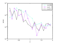
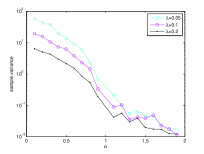
Fig. 3: Simulation results for Eq. (1.4). The left-hand plot (a) is for $|\mathrm{error}|$ (4.12), and the right-hand plot (b) for the sample variance.

Fig. 3 shows that the sample variances decrease with the increase of $\alpha$ and $\lambda$, and similarly $|\mathrm{error}|$ also tends to decrease. This figure also illustrates the effect of variance on the $\mathrm{error}$. Next, we show the influence of $n$ on the error.

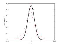
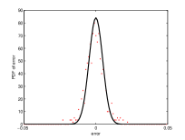
Fig. 4: Distribution of simulation errors for $\alpha=1.2$, $\lambda=0.05$, and $n=2000$ for (a) ($n=4000$ for (b)).

For fixed $n$, repeating the simulation $600$ times leads to the approximate distribution of errors. Figure  4 shows that the errors are normally distributed, where the real curve is the plot of the function $\left(2\pi\sigma^{2}/n\right)^{-0.5}\exp\left(-\frac{x^{2}}{2\sigma^{2}/n}\right)$ with $\sigma^{2}=0.1$ obtained from Fig. 3. Obviously the larger $n$ is, the smaller the variance of errors becomes. Figure 5 indicates the convergence of the algorithm, as expected, being $O(1/\sqrt{n})$.

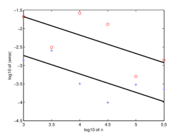
Fig. 5: Convergence of the simulations, respectively, with $\alpha=0.7,\lambda=0.2$ (red circle) and $\alpha=1.2,\lambda=0.05$ (blue plus ), when $n$ increases.

6 Conclusion

The first exit and Dirichlet problems for the nonisotropic tempered $\alpha$-stable process $X_{t}$ have been discussed. With the obtained upper bounds of all moments of the first exit position $\left|X_{\tau_{D}}\right|$ and the first exit time $\tau_{D}$, we show that the PDF of $\left|X_{\tau_{D}}\right|$ or $\tau_{D}$ exponentially decays with the increase of $\left|X_{\tau_{D}}\right|$ or $\tau_{D}$, and $\mathrm{E}\left[\tau_{D}\right]\sim\left|\mathrm{E}\left[X_{\tau_{D}}\right]\right|$, $\mathrm{E}\left[\tau_{D}\right]\sim\mathrm{E}\left[\left|X_{\tau_{D}}-\mathrm{E}\left[X_{\tau_{D}}\right]\right|^{2}\right]$. The Feynman-Kac representation is provided for the Dirichlet problem with the operator $\mathrm{\Delta}^{\alpha/2,\lambda}_{m}$, and some numerical simulations are performed to show its usefulness.

Appendix A Description for the algorithm of simulation

We work in two dimensions. Let $m(\theta)$ be the probability distribution of particles in $\theta$-direction, and $c_{m,\alpha}=\frac{1}{|\Gamma(-\alpha)|}$. Referring to 48 , we present the description of the algorithm.

For $0<\alpha<1$, set

$$S=\left(\Delta t\right)^{1/\alpha}\frac{\sin\alpha(U+\pi/2)}{\cos(U)^{1/\alpha}}\left(\frac{\cos\left(U-\alpha(U+\pi/2)\right)}{W}\right)^{(1-\alpha)\alpha},$$ (A.1)

where $U$ is an uniform distribution on $[-\pi/2,\pi/2]$, and $W$ is an exponential distribution with mean 1. Generate the random variable (r.v.) $Z$ of exponential distribution with mean $\lambda^{-1}$; if $Z<S$, reject and draw again, otherwise set $X_{\Delta t}=[S\cos\theta,S\sin\theta]$, where the r.v. $\theta$ is generated by the PDF $m(\theta)$.

When $1<\alpha<2$, set

$$S=\left(\Delta t\right)^{1/\alpha}\frac{\sin\alpha(U-\pi/2)}{\cos(U)^{1/\alpha}}\left(\frac{\cos\left(U-\alpha(U-\pi/2+\pi/\alpha)\right)}{W}\right)^{(1-\alpha)\alpha};$$ (A.2)

if $S>Z-b\,(b>0)$, reject and draw again, otherwise set $X_{\Delta t}=[S\cos\theta,S\sin\theta]$; again the PDF of $\theta$ is $m(\theta)$.

To simulate the entire path of the stable process, one can rewrite $X_{t}$ as follows

$$X_{t}=\sum^{t/{\Delta t}}_{i=1}\left[X_{i\Delta t}-X_{(i-1)\Delta t}\right].$$

The stationary and independent increments of $X_{t}$ show that

$$X_{i\Delta t}-X_{(i-1)\Delta t}\stackrel{{\scriptstyle d}}{{=}}X_{\Delta t}.$$

According to the above, one can generate the stochastic processes $X^{j}_{t}\,(j=1,2,\dots,n)$, which denotes the path of the $j$-th particle.

To calculate the PDF of $\tau_{D}$, divide the time interval $[0,T]$ into $m_{1}$ equal parts, i.e., $0=t_{0}<t_{1}<\dots<t_{m_{1}}=T,\,t_{i}=ih_{1}\,(i=0,1,\cdots,m_{1})$. Count the number $n_{1}^{i+1}$ of particles, the time of which spend on lies in the interval $(t_{i},t_{i+1}]$ when firstly leaving the domain $B(0,r)$. Then, $\frac{n_{1}^{i+1}}{nh_{1}}$ denotes the PDF of $\tau_{D}$ in $(t_{i},t_{i+1}]$.

To calculate the PDF of $|X_{\tau_{D}}|$, divide the interval $(r,l]$ into $m_{2}$ equal parts, i.e., $r=r_{0}<r_{1}<\cdots<r_{m_{2}}=l,r_{i}=ih_{2}+r_{0}\,(i=0,1,\cdots,m_{2})$. Count the number $n_{2}^{i+1}$ of particles that fall into the annular region $(r_{i},r_{i+1}]$, when first exiting the domain $B(0,r)$. Then, $\frac{n_{2}^{i+1}}{nh_{2}}$ denotes the PDF of $|X_{\tau_{D}}|$ in $(r_{i},r_{i+1}]$.

References

(1)W. H. Deng, B. Y. Li, W. Y. Tian and P. W. Zhang.: Boundary problems for the fractional and tempered fractional operators. Multiscale Model. Simul. 16(1), 125-149 (2018).
(2)D. Applebaum.: Lévy processes and stochastic calculus. Cambridge University Press, Cambridge, second ed (2009).
(3)J. F. Kelly, C. C. Li and M. M. Meerschaert.: Anomalous diffusion with ballistic scaling: A new fractional derivative. J. Comput. Appl. Math. 339, 161-178 (2018).
(4)S. Jin and B. Yan.: A class of asymptotic-preserving schemes for the Fokker-Planck-Landau equation. J.
Comput. Phys. 230(17), 6420-6437 (2011).
(5)F. Filbet and L. Pareschi.: A numerical method for the accurate solution of the Fokker-Planck-Landau equation in the nonhomogeneous case. J. Comput. Phys. 179(1), 1-26 (2002).
(6)R. Metzler and J. Klafter.: The random walk’s guide to anomalous diffusion: a fractional dynamics approach. Phys. Rep. 339(1), 1-77 (2000).
(7)P. D. Ditlevsen.: Observation of -stable noise induced millennial climate changes from an ice-core record. Res. Lett. 26(10), 1441-1444 (1999).
(8)D. Brockmann, L. Hufnagel and T. Geisel.: The scaling laws of human travel. Nature. 439(7075), 462-465 (2006).
(9)B. Dybiec, A. Kleczkowski and C. A. Gilligan.: Modelling control of epidemics spreading by long-range interactions. J. R. Soc. Interface. 52(4), 2462-2473 (2016).
(10)Y. Zhang, M. M. Meerschaert and R. M. Neupauer.: Backward fractional advection dispersion model for contaminant source prediction. Water Resour. Res. 6(39), 941-950 (2009).
(11)S. Redner.: A guide to first passage time processes. Cambridge University, Cambridge (2001).
(12)W. H. Deng, X. C. Wu and W. L. Wang.: Mean exit time and escape probability for the anomalous processes with the tempered power-law waiting times. EPL. 117(1), 10009 (2017).
(13)A. N. Borodin and P. Salminen.: Handbook of brownian motion: facts and formulae. Birkhuser, Basel, second ed (2002).
(14)D. R. Cox and H. D. Miller.: The Theory of Stochastic Processes. Chapman and Hall, London (1965).
(15)J. Klafter, S. C. Lim and R. Metzler.: Fractional Dynamics: Recent Advances. World Scientific, Singapore (2012).
(16)B. Dybiec, E. Gudowska-Nowak and P. Hnggi.: Lévy-Brownian motion on finite intervals: Mean first passage time analysis. Phys. Rev. E. 73(4), 046104 (2006).
(17)A. Zoia, A. Rosso and M. Kardar.: Fractional Laplacian in bounded domains. Phys. Rev. E. 76(2), 021116 (2007).
(18)T. Koren, M. A. Lomholt, A. V. Chechkin, J. Klafter and R. Metzler.: Leapover lengths and first passage time statistics for Lévy flights. Phys. Rev. Lett. 99(16), 160602 (2007).
(19)T. Koren, A. V. Chechkin and J. Klafter.: On the first passage time and leapover properties of Lévy motions. Physica A. 379(1), 10-22 (2007).
(20)E. Martin, U. Behn and G. Germano.: First-passage and first-exit times of a Bessel-like stochastic process. Phys. Rev. E. 83(5), 051115 (2011).
(21)I. Eliazar and J. Klafter.: On the first passage of one-sided Lévy motions. Physica A. 336(3-4), 219-244 (2004).
(22)G. Bel and E. Barkai.: Random walk to a nonergodic equilibrium concept. Phys. Rev. E. 73(1), 016125 (2006).
(23)J. Gajda and M. Magdziarz.: Kramers escape problem for fractional Klein-Kramers equation with tempered
-stable waiting times. Phys. Rev. E. 84(2), 021137 (2011).
(24)H. C. Fogedby.: Langevin equations for continuous time Lévy flights. Phys. Rev. E. 50(2), 1657 (1994).
(25)R. K. Getoor.: First passage times for symmetric stable processes in space. Trans. Am. Math. Soc. 101(1), 75-90 (1961).
(26)S. V. Buldyrev, S. Havlin, A. Ya. Kazakov, M. G. E. da Luz, E. P. Raposo, H. E. Stanley and G. M. Viswanathan.: Average time spent by Lévy flights and walks on an interval with absorbing boundaries. Phys. Rev. E. 64(4), 041108 (2001).
(27)J. A. Given, C. O. Hwang and M. Mascagni.: First-and last-passage Monte Carlo algorithms for the charge density distribution on a conducting surface. Phys. Rev. E. 66, 056704 (2002).
(28)K. Szczepaniec and B. Dybiec.: Escape from bounded domains driven by multivariate -stable noises. J. Stat. Mech. 2015(6), P06031 (2015).
(29)R. M. Blumenthal, R. K. Getoor and D. B. Ray.: On the distribution of first hits for the symmetric stable processes. Trans. Am. Math. Soc. 99(3), 540-554 (1961).
(30)G. Acosta and J. P. Borthagaray.: A fractional Laplace equation: Regularity of solutions
and finite element approximations. SIAM J. Numer. Anal. 55(2), 472-495 (2017).
(31)Y. Huang and A. M. Oberman.: Numerical methods for the fractional Laplacian: A finite difference-quadrature approach. SIAM J. Numer. Anal. 52(6), 3056-3084 (2014).
(32)M. D’Elia and M. Gunzburger.: The fractional Laplacian operator on bounded domains
as a special case of the nonlocal diffusion operator. Comp. Math. Appl. 66(7), 1245-1260 (2013).
(33)J. P. Borthagaray, L. M. Del Pezzo and S. Martínez.: Finite element approximation
for the fractional eigenvalue problem. J. Sci. Comput. 77(1), 308-329 (2018).
(34)G. Acosta, F. Bersetche and J. P. Borthagaray.: A short FEM implementation for a 2d homogeneous Dirichlet problem of a fractional Laplacian. Comput. Math. Appl. 74(4), 784-816 (2017).
(35)K. Bogdan and T. Byczkowski.: Potential theory for the -stable Schrdinger operator on bounded Lipschitz domains. Studia Math. 133(1), 53-92 (1999)
(36)A. E. Kyprianou, A. Osojnik and T. Shardlow.: Unbiased ‘walk-on-spheres’ Monte Carlo methods
for the fractional Laplacian. IMA J. Numer. Anal. 38(3), 1550-1578 (2018).
(37)M. E. Muller.: Some continuous Monte Carlo methods for the Dirichlet problem. Ann. Math. Statist. 27(3), 569-589 (1956).
(38)I. Dimov and O. Tonev.: Random walk on distant mesh points Monte Carlo methods. J. Stat. Phys. 70(5-6), 1333-1342 (1993).
(39)G. A. Mikhailov.: Solving the Dirichlet problem for nonlinear elliptic equations by the Monte Carlo method. Siberian Math. J. 35(5), 967-975 (1994).
(40)P. Baldi.: Exact asymptotics for the probability of exit from a domain and applications to simulation. Ann. Probab. 23(4), 1644-1670 (1995).
(41)J. A. Acebroön, M. P. Busico, P. Lanucara and R. Spigler.: Domain decomposition solution of elliptic boundary-value problems via Monte Carlo and quasi-Monte Carlo methods. SIAM J. Sci. Comput. 27(2), 440-457 (2005).
(42)A. L. Teckentrup, R. Scheichl, M. B. Giles and E. Ullmann.: Further analysis of multilevel Monte Carlo methods for elliptic PDEs with random coefficients. Numer. Math. 125(3), 569-600 (2013).
(43)W. H. Deng, X. D. Wang and P. W. Zhang: Nonlocal diffusion operators for normal and anomalous dynamics. arXiv:1805.00653v1, (2018).
(44)M. M. Meerschaert and A. Sikorskii.: Stochastic models for fractional calculus. Walter de Gruyter GmbH & Co. KG, Berlin (2012).
(45)W. E. Pruitt.: The growth of random walks and Lévy processes. Ann. Probab. 9(6), 948-956 (1981).
(46)P. S. Griffin and T. R. McConnell.: On the position of a random walk at the time of first exit from a sphere. Ann. Probab. 20(2), 825-854 (1992).
(47)Y. S. Chow and H. Teicher.: Probability theory. Springer, New York, second ed (1978).
(48)B. Baeumer and M. M. Meerschaert.: Tempered stable Lévy motion and transient super-diffusion. J. Comput. Appl. Math. Simul. 233(10), 2438-2448 (2010).