Strong convergence of the linear implicit Euler method for the finite element discretization of semilinear non-autonomous SPDEs driven by multiplicative or additive noise

Abstract

This paper aims to investigate the numerical approximation of semilinear non-autonomous stochastic partial differential equations (SPDEs) driven by multiplicative or additive noise. Such equations are more realistic than the autonomous ones when modeling real world phenomena. Such equations find applications in many fields such as transport in porous media, quantum fields theory, electromagnetism and nuclear physics. Numerical approximations of autonomous SPDEs are thoroughly investigated in the literature, while the non-autonomous case is not yet well understood. Here, a non-autonomous SPDE is discretized in space by the finite element method and in time by the linear implicit Euler method. We break the complexity in the analysis of the time depending, not necessarily self-adjoint linear operators with the corresponding semigroup and provide the strong convergence result of the fully discrete scheme toward the mild solution. The results indicate how the converge order depends on the regularity of the initial solution and the noise. Additionally, for additive noise we achieve convergence order in time approximately $1$ under less regularity assumptions on the nonlinear drift term than required in the current literature, even in the autonomous case. Numerical simulations motivated from realistic porous media flow are provided to illustrate our theoretical finding.

1 Introduction

We consider numerical approximation of the following non-autonomous SPDE defined in $\Lambda\subset\mathbb{R}^{d}$, $d=\{1,2,3\}$ (where $\Lambda$ is bounded with smooth boundary),

$$dX(t)+A(t)X(t)dt=F(t,X(t))dt+B(t,X(t))dW(t),\quad t\in(0,T],\quad X(0)=X_{0},$$ (1)

on the Hilbert space $L^{2}(\Lambda,\mathbb{R})$, $T>0$ is the final time, $F$ and $B$ are nonlinear functions and $X_{0}$ is the initial data, which is random. The family of linear operators $A(t)$ are unbounded, not necessarily self-adjoint, and for all $s\in[0,T]$, $-A(s)$ is the generator of an analytic semigroup $S_{s}(t)=:e^{-tA(s)},t\geq 0.$ The noise $W(t)$ is a $Q-$Wiener process defined in a filtered probability space $(\Omega,\mathcal{F},\mathbb{P},\{\mathcal{F}_{t}\}_{t\geq 0})$. The filtration is assumed to fulfill the usual conditions (see e.g. [38, Definition 2.1.11]). Note that the noise can be represented as follows (see e.g. [38, 37])

$$W(x,t)=\sum_{i\in\mathbb{N}^{d}}\sqrt{q_{i}}e_{i}(x)\beta_{i}(t),\quad t\in[0,T],\quad x\in\Lambda,$$ (2)

where $q_{i}$, $e_{i}$, $i\in\mathbb{N}^{d}$ are respectively the eigenvalues and the eigenfunctions of the covariance operator $Q$, and $\beta_{i}$, $i\in\mathbb{N}$, are independent and identically distributed standard Brownian motions. Precise assumptions on $F$, $B$, $X_{0}$ and $A(t)$ will be given in the next section to ensure the existence of the unique mild solution $X$ of (1). In many situations it is hard to exhibit explicit solutions of SPDEs. Therefore, numerical algorithms are good tools to provide realistic approximations. Strong approximations of autonomous SPDEs with constant linear self-adjoint operator $A(t)=A$ are widely investigated in the literature, see e.g. [47, 46, 20, 17, 25, 48] and references therein. When we turn our attention to the case of semilinear SPDEs, still with constant operator $A(t)=A$, but not necessary self-adjoint, the list of references becomes remarkably short, see e.g. [24, 31]. Note that modelling real world phenomena with time dependent linear operator is more realistic than modelling with time independent linear operator (see e.g. [4] and references therein). The deterministic counterpart of (1) finds applications in many fields such as quantum fields theory, electromagnetism, nuclear physics and transport in porous media. To the best of our knowledge, numerical approximations of non-autonomous SPDEs are not yet well understood in the literature due to the complexity of the linear operator $A(t)$, its semigroup $S_{t}(s)$ and the resolvent operator $(\mathbf{I}+tA(s))^{-1}$, $t,s\in[0,T]$. Our aims is to fill that gap in this paper and in our accompanied papers [43, 32]. The Magnus-type integrators are developed in the accompanied papers [43, 32] for SPDEs with multiplicative and additive noise. Magnus-type integrators use the fact that the solution of the deterministic system of differential equations $y^{\prime}(t)=A(t)y(t)$ can be represented in the following exponential form $y(t)=\exp(\Gamma(t))y(0)$ (see e.g. [28, 2, 3]), where $\Gamma(t)$ is called Magnus expansion or Magnus series. Note that the Magnus series does not always converges. One sufficient condition for its convergence is: $\int_{0}^{T}\|A(t)\|_{2}dt<\pi$ (see e.g. [30, 28] or [12, Section IV.7]), where $\|.\|_{2}$ stands for the matrix norm. For some problems with large $\|A(t)\|_{2}$, the Magnus series seems to diverge (see e.g. [11]). Hence, for such problems, it is important to find alternative numerical schemes. In this paper, we develop an alternative method based on linear implicit method, which does not make use of the Magnus series and which is more stable than the explicit Magnus-type integrators developed in [43, 32]. The space discretization is performed using the finite element method. Note that the implementation of this method is based on the resolution of linear systems and may be more efficient than Magnus-type integrators when the appropriate preconditioners are used. Here, we break the complexity in the analysis of the time depending, not necessarily self-adjoint linear operators with the corresponding semigroup and provide the strong convergence results of the fully discrete schemes toward the exact solution in the root-mean-square $L^{2}$ norm. The main challenge here is that the resolvent operators change at each time step. So novel stability estimates, useful in the convergence analysis are needed. These novel estimates are provided in Section 3.1. Note that the preparatory results in Section 3.1 are different from results in [43, 32] and are very challenging.

• In fact, here the key ingredient is the discrepancy between the two parameters semigroup $U_{h}(t,s)$ and the resolvent operator $\left(\mathbf{I}+\Delta tA_{h}(t_{j})\right)^{-1}$, which is much more complicated than estimating the discrepancy between $U_{h}(t,s)$ and its approximated form $e^{A_{h}(s)(t-s)}$, which was one of the core of works in [43, 32].

• Note that even in the autonomous case, the discrepancy between the semigroup $S(t)$ and the resolvent operator $(\mathbf{I}+\Delta tA)^{-1}$ is a key ingredient in approximating SPDEs with linear implicit method. Such discrepancy for smooth and non smooth initial data with linear constant self adjoint operator $A$ were done in [45, Theorem 7.8] and [45, Theorem 7.7] respectively, where authors used the spectral decomposition of $A$. In fact, [45, Theorem 7.8] and [45, Theorem 7.7] are key ingredients in the literature when analyzing convergence of autonomous SPDEs via linear implicit method, see e.g. [46, 20, 25].

• In the case of non-autonoumous SPDEs, [45, Theorem 7.8] and [45, Theorem 7.7] are no longer applicable and to prove their analogous for time dependent operator, one cannot just follow the steps of the proofs of [45, Theorem 7.8] and [45, Theorem 7.7], since in this case, in addition to the fact that the operators $A(t)$ are changing at each time step, they are not self adjoint and therefore the spectral decomposition is not applicable. Section 3.1 (more precisely Lemmas 3.8 and 3.9) uses an argument based on telescopic sums and provides key ingredients to handle these challenges.

• Moreover, in comparison to many works in the literature for additive noise, where the authors achieved convergence order in time approximately $1$ (see e.g. [46, 25]), we also achieve similar convergence order, but with less regularity assumptions on the nonlinear drift function, which extends the class of the nemytskii operaor $F$. In fact, we only require $F$ to be differentiable with Lipschitz continuous derivative, while in the up to date literature (see e.g. [46, 25, 47]) the authors requires the derivatives up to order $2$ to be bounded. This is restrictive and exclude many Nemytskii operators such as $F(u)=\frac{|u|}{1+u^{2}}$, $u\in H$. In fact, the later function $F$ does not even have a second derivative at $0$.

Our rigorous mathematical analysis shows how the convergence rates depend on the regularity of the initial data and the noise. In fact, we achieve convergence orders $\mathcal{O}\left(h^{\beta}+\Delta t^{\frac{\min(\beta,1)}{2}}\right)$ for multiplicative noise and $\mathcal{O}\left(h^{\beta}+\Delta t^{\frac{\beta}{2}-\epsilon}\right)$ for additive noise, where $\beta$ is the regularity parameter from Assumption 2.1 and $\epsilon$ is a positive number small enough.

The rest of this paper is organized as follows: Section 2 deals with the well posedness problem, the numerical scheme and the main results. In section 3, we provide some errors estimates for the corresponding deterministic homogeneous problem as preparatory results along with the proofs of the main results. Section 4 provides some numerical experiments motivated from realistic porous media to sustain the theoretical findings.

2 Mathematical setting and main results

2.1 Main assumptions and well posedness problem

Let $(H,\langle.,.\rangle,\|.\|)$ be a separable Hilbert space. For any $p\geq 2$ and for a Banach space $U$, we denote by $L^{p}(\Omega,U)$ the Banach space of all equivalence classes of $p$ integrable $U$-valued random variables. Let $L(U,H)$ be the space of bounded linear mappings from $U$ to $H$ endowed with the usual operator norm $\|.\|_{L(U,H)}$. By $\mathcal{L}_{2}(U,H):=HS(U,H)$, we denote the space of Hilbert-Schmidt operators from $U$ to $H$ equipped with the norm $\|l\|^{2}_{\mathcal{L}_{2}(U,H)}:=\sum\limits_{i=1}^{\infty}\|l\psi_{i}\|^{2}$, $l\in\mathcal{L}_{2}(U,H)$, where $(\psi_{i})_{i=1}^{\infty}$ is an orthonormal basis of $U$. Note that this definition is independent of the orthonormal basis of $U$. For simplicity, we use the notations $L(U,U)=:L(U)$ and $\mathcal{L}_{2}(U,U)=:\mathcal{L}_{2}(U)$. For all $l\in L(U,H)$ and $l_{1}\in\mathcal{L}_{2}(U)$, it holds that

$$ll_{1}\in\mathcal{L}_{2}(U,H)\quad\text{and}\quad\|ll_{1}\|_{\mathcal{L}_{2}(U,H)}\leq\|l\|_{L(U,H)}\|l_{1}\|_{\mathcal{L}_{2}(U)},$$ (3)

see e.g. [5]. The covariance operator $Q:H\longrightarrow H$ is assumed to be positive definite and self-adjoint. The space of Hilbert-Schmidt operators from $Q^{\frac{1}{2}}(H)$ to $H$ is denoted by $L^{0}_{2}:=\mathcal{L}_{2}(Q^{\frac{1}{2}}(H),H)=HS(Q^{\frac{1}{2}}(H),H)$. As usual, $L^{0}_{2}$ is equipped with the norm $\|l\|_{L^{0}_{2}}:=\|lQ^{\frac{1}{2}}\|_{HS}=\left(\sum\limits_{i=1}^{\infty}\|lQ^{\frac{1}{2}}e_{i}\|^{2}\right)^{\frac{1}{2}},\quad l\in L^{0}_{2}$, where $(e_{i})_{i=1}^{\infty}$ is an orthonormal basis of $H$. This definition is independent of the orthonormal basis of $H$.

For an $L^{0}_{2}$- predictable stochastic process $\phi:[0,T]\times\Lambda\longrightarrow L^{0}_{2}$ such that

$$\int_{0}^{t}\mathbb{E}\left\|\phi(s)Q^{\frac{1}{2}}\right\|^{2}_{\mathcal{L}_{2}(H)}ds<\infty,\quad t\in[0,T],$$

the following relation called Itô’s isometry holds

$$\mathbb{E}\left\|\int_{0}^{t}\phi(s)dW(s)\right\|^{2}=\int_{0}^{t}\mathbb{E}\|\phi(s)\|^{2}_{L^{0}_{2}}ds=\int_{0}^{t}\mathbb{E}\left\|\phi(s)Q^{\frac{1}{2}}\right\|^{2}_{\mathcal{L}_{2}(H)}ds,\quad t\in[0,T],$$ (4)

see e.g. [37, Step 2 in Section 2.3.2] or [38, Proposition 2.3.5].

In the rest of this paper, we consider $H=L^{2}(\Lambda,\mathbb{R})$. To guarantee the existence of a unique mild solution of (1) and for the purpose of the convergence analysis, we make the following assumptions.

Assumption 2.1

The initial data $X_{0}:\Omega\longrightarrow H$ is assumed to be measurable and belongs to $L^{2}\left(\Omega,\mathcal{D}\left(\left(A(0)\right)^{\frac{\beta}{2}}\right)\right)$, with $0\leq\beta\leq 2.$

Assumption 2.2

• As in [11, 14, 43, 41], we assume that $\mathcal{D}(A(t))=D$, $0\leq t\leq T$ and that the family of linear operators $A(t):D\subset H\longrightarrow H$ is uniformly sectorial on $0\leq t\leq T$, i.e. there exist constants $c>0$ and $\theta\in(\frac{1}{2}\pi,\pi)$ such that

  $$\|(\lambda\mathbf{I}-A(t))^{-1}\|_{L(L^{2}(\Lambda))}\leq\frac{c}{|\lambda|},\quad\lambda\in S_{\theta},$$

  where $S_{\theta}:=\{\lambda\in\mathbb{C}:\lambda=\rho e^{i\phi},\rho>0,0\leq|\phi|\leq\theta\}$. As in [14], by a standard scaling argument, we assume $-A(t)$ to be invertible with bounded inverse.

• As in [14, 11], we require the following Lipschitz conditions: there exists a positive constant $K_{1}$ such that

  $$\left\|\left(A(t)-A(s)\right)(A(0))^{-1}\right\|_{L(H)} \leq K_{1}|t-s|,\quad s,t\in[0,T],$$ (5)

  $$\left\|(A(0))^{-1}\left(A(t)-A(s)\right)\right\|_{L(D,H)} \leq K_{1}|t-s|,\quad s,t\in[0,T].$$ (6)

• Since we are dealing with non smooth data, we follow [41, 43] and assume that

  $$\mathcal{D}((A(t))^{\alpha})=\mathcal{D}((A(0))^{\alpha}),\quad 0\leq t\leq T,\quad\alpha\in[0,1]$$ (7)

  and there exists a positive constant $K_{2}$ such that the following estimate holds

  $$K_{2}^{-1}\|(A(0))^{\alpha}u\|\leq\|(A(t))^{\alpha}u\|\leq K_{2}\|(A(0))^{\alpha}u\|,\quad u\in D\left((A(0))^{\alpha}\right),\quad t\in[0,T].$$ (8)

Remark 2.1

As a consequence of Assumption 2.2, for all $\alpha\geq 0$ and $\gamma\in[0,1]$, there exists a constant $C_{1}>0$ such that the following estimates hold uniformly in $t\in[0,T]$

$$\left\|(A(t))^{\alpha}e^{-sA(t)}\right\|_{L(H)}\leq C_{1}s^{-\alpha},s>0,\quad\left\|(A(t))^{-\gamma}\left(\mathbf{I}-e^{-rA(t)}\right)\right\|_{L(H)}\leq C_{1}r^{\gamma},\quad r\geq 0.$$ (9)

Remark 2.2

Let $\Delta(T):=\{(t,s):0\leq s\leq t\leq T\}$. It is well known [36, Theorem 6.1, Chapter 5] that under Assumption 2.1 there exists a unique evolution system [36, Definition 5.3, Chapter 5] $U:\Delta(T)\longrightarrow L(H)$ satisfying:

• there exists a positive constant $K_{0}$ such that

  $$\|U(t,s)\|_{L(H)}\leq K_{0},\quad 0\leq s\leq t\leq T.$$

• $U(.,s)\in C^{1}(]s,T];L(H))$, $0\leq s\leq T$,

  $$\frac{\partial U}{\partial t}(t,s)=A(t)U(t,s),\quad\|A(t)U(t,s)\|_{L(H)}\leq\frac{K_{0}}{t-s},\quad 0\leq s<t\leq T.$$

• $U(t,.)v\in C^{1}([0,t[;H)$, $0<t\leq T$, $v\in\mathcal{D}(A(0))$ and

  $$\frac{\partial U}{\partial s}(t,s)v=-U(t,s)A(s)v,\quad\|A(t)U(t,s)A(s)^{-1}\|_{L(H)}\leq K_{0},\quad 0\leq s\leq t\leq T.$$

We equip $V_{\alpha}(t):=\mathcal{D}((A(t))^{\frac{\alpha}{2}})$, $\alpha\in\mathbb{R}$ with the norm $\|u\|_{\alpha,t}:=\|(A(t))^{\frac{\alpha}{2}}u\|$. Due to (7), (8) and for the seek of ease notations, we simply write $V_{\alpha}$ and $\|.\|_{\alpha}$.

We follow [41, 43] and make the following assumptions on operators $F$ and $B$.

Assumption 2.3

The nonlinear operator $F:[0,T]\times H\longrightarrow H$ is $\frac{\beta}{2}$-Hölder continuous with respect to the first variable and Lipschitz continuous with respect to the second variable, i.e. there exists a positive constant $K_{3}$ such that

$$\|F(s,0)\|\leq K_{3},\quad\|F(t,u)-F(s,v)\|\leq K_{3}\left(|t-s|^{\frac{\beta}{2}}+\|u-v\|\right),\;s,t\in[0,T],\;u,v\in H.$$

Assumption 2.4

The diffusion coefficient $B:[0,T]\times H\longrightarrow L^{0}_{2}$ is $\frac{\beta}{2}$-Hölder continuous with respect to the first variable and Lipschitz continuous with respect to the second variable, i.e. there exists a positive constant $K_{4}$ such that

$$\|B(s,0)\|_{L^{0}_{2}}\leq K_{4},\quad\|B(t,u)-B(s,v)\|_{L^{0}_{2}}\leq K_{4}\left(|t-s|^{\frac{\beta}{2}}+\|u-v\|\right),\;s,t\in[0,T],\,u,v\in H.$$

To establish our $L^{2}$ strong convergence result when dealing with multiplicative noise, we will also need the following further assumption on the diffusion term when $\beta\in[1,2)$, which was also used in [19, 21] to achieve optimal regularities, and in [24, 20, 31, 42] to achieve optimal convergence orders in space and in time.

Assumption 2.5

We assume that $B\left(\mathcal{D}\left(A(0)^{\frac{\beta-1}{2}}\right)\right)\subset HS\left(Q^{\frac{1}{2}}(H),\mathcal{D}\left(A(0)^{\frac{\beta-1}{2}}\right)\right)$ and there exists $c\geq 0$ such that for all $v\in\mathcal{D}\left(A(0)^{\frac{\beta-1}{2}}\right)$, $\left\|A(0)^{\frac{\beta-1}{2}}B(v)\right\|_{L^{0}_{2}}\leq c\left(1+\|v\|_{\beta-1}\right)$, where $\beta$ is the parameter defined in Assumption 2.1.

Typical examples which fulfill Assumption 2.5 are stochastic reaction diffusion equations (see e.g. [19, Section 4]).

For additive noise, we make the following assumption on the covariance operator.

Assumption 2.6

We assume that the covariance operator $Q:H\longrightarrow H$ satisfies

$$\left\|(A(0))^{\frac{\beta-1}{2}}Q^{\frac{1}{2}}\right\|_{\mathcal{L}_{2}(H)}<\infty,$$

where $\beta$ is defined in Assumption 2.1.

In order to achieve convergence order greater than $\frac{1}{2}$ when dealing with additive noise, we require the following assumption on $F$, which is less restrictive than those used in [31, 47, 46, 43, 42] and hence includes many nonlinear drift functions.

Assumption 2.7

The nonlinear function $F:[0,T]\times H\longrightarrow H$ is differentiable with respect to the second variable and there exists $C_{2}\geq 0$ such that

$$\|F^{\prime}(t,u)v\|\leq C_{2}\|v\|,\quad\|A^{-\frac{\eta}{2}}\left(F^{\prime}(t,u)-F^{\prime}(t,v)\right)\|_{L(H)}\leq C\|u-v\|,\quad t\in[0,T],\;u,v\in H,$$

for some $\eta\in(\frac{3}{4},1)$, where $F^{\prime}(t,u)=\frac{\partial F}{\partial u}(t,u)$ for $t\in[0,T]$ and $u\in H$.

Theorem 2.1

[41, Theorem 1.3] Let Assumptions 2.2 (i)-(ii), 2.1, 2.3 and 2.4, be fulfilled. Then the non-autonomous problem (1) has a unique mild solution $X(t)$, which takes the following integral form

$$X(t)=U(t,0)X_{0}+\int_{0}^{t}U(t,s)F(s,X(s))ds+\int_{0}^{t}U(t,s)B(s,X(s))dW(s),\quad t\in[0,T],$$ (10)

where $U(t,s)$ is the evolution system defined in Remark 2.2. Moreover, there exists a positive constant $K_{5}$ such that

$$\sup_{0\leq t\leq T}\|X(t)\|_{L^{2}\left(\Omega,\mathcal{D}\left((-A(0))^{\frac{\beta}{2}}\right)\right)}\leq K_{5}\left(1+\|X_{0}\|_{L^{2}\left(\Omega,\mathcal{D}\left((-A(0))^{\frac{\beta}{2}}\right)\right)}\right).$$ (11)

2.2 Numerical scheme and main results

For the seek of simplicity, we consider the family of linear operators $A(t)$ to be of second order and has the following form

$$A(t)u=-\sum_{i,j=1}^{d}\frac{\partial}{\partial x_{i}}\left(q_{i,j}(x,t)\frac{\partial u}{\partial x_{j}}\right)+\sum_{j=1}^{d}q_{j}(x,t)\frac{\partial u}{\partial x_{j}}.$$ (12)

We require the coefficients $q_{i,j}$ and $q_{j}$ to be smooth functions of the variable $x\in\overline{\Lambda}$ and Hölder-continuous with respect to $t\in[0,T]$. We further assume that there exists a positive constant $c$ such that the following ellipticity condition holds

$$\sum_{i,j=1}^{d}q_{i,j}(x,t)\xi_{i}\xi_{j}\geq c|\xi|^{2},\quad(x,t)\in\overline{\Lambda}\times[0,T].$$ (13)

Under the above assumptions on $q_{i,j}$ and $q_{j}$, it is well known that the family of linear operators defined by (12) fulfils Assumption 2.2 (i)-(ii), see e.g. [10, Chapter III, Section 11], [36, Section 7.6] or [44, Section 5.2]. The above assumptions on $q_{i,j}$ and $q_{j}$ also imply that Assumption 2.2 (iii) is fulfilled, see e.g. [41, Example 6.1], [10, Chapter III] or [1, 40]. In the abstract form (1), the nonlinear functions $F:[0,T]\times H\longrightarrow H$ and $B:[0,T]\times H\longrightarrow HS(Q^{\frac{1}{2}}(H),H)$ are defined by

$$(F(t,v))(x)=f(t,x,v(x)),\quad(B(t,v)u)(x)=b(t,x,v(x)).u(x),\quad x\in\Lambda,\quad v\in H,$$ (14)

$u\in Q^{\frac{1}{2}}(H)$, $t\in[0,T]$, where $f:\mathbb{R}_{+}\times\Lambda\times\mathbb{R}\longrightarrow\mathbb{R}$ and $b:\mathbb{R}_{+}\times\Lambda\times\mathbb{R}\longrightarrow\mathbb{R}$ are continuously differentiable functions with globally bounded derivatives. As in [10, 24], we introduce two spaces $\mathbb{H}$ and $V$, such that $\mathbb{H}\subset V$, that depend on the boundary conditions for the domain of the operator $A(t)$ and the corresponding bilinear form. For example, for Dirichlet boundary conditions we introduce the following space

$$V=H^{1}_{0}(\Lambda)=\{v\in H^{1}(\Lambda):v=0\quad\text{on}\quad\partial\Lambda\}.$$

For Robin boundary conditions and Neumann boundary conditions, which is a special case of Robin boundary conditions ($\alpha_{0}=0$), we take $V=H^{1}(\Lambda)$ and

$$\mathbb{H}=\{v\in H^{2}(\Lambda):\partial v/\partial v_{A}+\alpha_{0}v=0,\quad\text{on}\quad\partial\Lambda\},\quad\alpha_{0}\in\mathbb{R}.$$

Using Green’s formula and the boundary conditions, we obtain the associated bilinear form to $A(t)$

$$a(t)(u,v)=\int_{\Lambda}\left(\sum_{i,j=1}^{d}q_{ij}(x,t)\dfrac{\partial u}{\partial x_{i}}\dfrac{\partial v}{\partial x_{j}}+\sum_{i=1}^{d}q_{i}(x,t)\dfrac{\partial u}{\partial x_{i}}v\right)dx,\quad u,v\in V,$$

for Dirichlet and Neumann boundary conditions and

$$a(t)(u,v)=\int_{\Lambda}\left(\sum_{i,j=1}^{d}q_{ij}(x,t)\dfrac{\partial u}{\partial x_{i}}\dfrac{\partial v}{\partial x_{j}}+\sum_{i=1}^{d}q_{i}(x,t)\dfrac{\partial u}{\partial x_{i}}v\right)dx+\int_{\partial\Lambda}\alpha_{0}uvdx,\quad u,v\in V.$$

for Robin boundary conditions. Using Gårding’s inequality (see e.g. [45, (4.3)]) yields

$$a(t)(v,v)\geq\lambda_{0}\|v\|^{2}_{1}-c_{0}\|v\|^{2},\quad v\in V,\quad t\in[0,T].$$

By adding and subtracting $c_{0}X$ on the right hand side of (1), we obtain a new family of linear operators that we still denote by $A(t)$. Therefore the new corresponding bilinear form associated to $A(t)$ still denoted by $a(t)$ satisfies the following coercivity property

$$a(t)(v,v)\geq\;\lambda_{0}\|v\|_{1}^{2},\;\;\;\;\;v\in V,\quad t\in[0,T].$$ (15)

Note that the expression of the nonlinear term $F$ has changed as we have included the term $-c_{0}X$ in the new nonlinear term that we still denoted by $F$.

The coercivity property (15) implies that $A(t)$, $t\in[0,T]$ is sectorial on $L^{2}(\Lambda)$, see e.g., [23]. Therefore $-A(t)$, $t\in[0,T]$ generates an analytic semigroups denoted by $S_{t}(s)=:e^{-sA(t)}$ on $L^{2}(\Lambda)$ such that [13]

$$S_{t}(s):=e^{-sA(t)}=\dfrac{1}{2\pi i}\int_{\mathcal{C}}e^{s\lambda}(\lambda I-A(t))^{-1}d\lambda,\quad\;s>0,$$

where $\mathcal{C}$ denotes a path that surrounds the spectrum of $-A(t)$. The coercivity property (15) also implies that $A(t)$ is a positive operator and its fractional powers are well defined and for any $\alpha>0$ we have

$$\left\{\begin{array}[]{rcl}(A(t))^{-\alpha}&=&\frac{1}{\Gamma(\alpha)}\displaystyle\int_{0}^{\infty}s^{\alpha-1}{\rm e}^{-sA(t)}ds,\\ (A(t))^{\alpha}&=&((A(t))^{-\alpha})^{-1},\end{array}\right.$$ (16)

where $\Gamma(\alpha)$ is the Gamma function (see [13]). The domain of $(A(t))^{\frac{\alpha}{2}}$ are characterized in [10, 7, 23] for $1\leq\alpha\leq 2$ with equivalence of norms as follows:

$$\mathcal{D}((A(t))^{\frac{\alpha}{2}})=H^{1}_{0}(\Lambda)\cap H^{\alpha}(\Lambda)\hskip 28.45274pt\text{(for Dirichlet boundary condition)}$$

$$\mathcal{D}(A(t))=\mathbb{H},\quad\mathcal{D}((A(t))^{\frac{1}{2}})=H^{1}(\Lambda)\hskip 14.22636pt\text{(for Robin boundary condition)}$$

$$\|v\|_{H^{\alpha}(\Lambda)}\equiv\|((A(t))^{\frac{\alpha}{2}}v\|:=\|v\|_{\alpha,t},\quad v\in\mathcal{D}((A(t))^{\frac{\alpha}{2}}).$$

The characterization of $\mathcal{D}((A(t))^{\frac{\alpha}{2}})$ for $0\leq\alpha<1$ can be found in [34, Theorems 2.1 & 2.2].

Now, we turn our attention to the discretization of the problem (1). We start by splitting the domain $\Lambda$ in finite triangles. Let $\mathcal{T}_{h}$ be the triangulation with maximal length $h$ satisfying the usual regularity assumptions, and $V_{h}\subset V$ be the space of continuous functions that are piecewise linear over the triangulation $\mathcal{T}_{h}$. We consider the projection $P_{h}$ from $H=L^{2}(\Lambda)$ to $V_{h}$ defined for every $u\in H$ by

$$\langle P_{h}u,\chi\rangle=\langle u,\chi\rangle,\quad\phi,\chi\in V_{h}.$$ (17)

For all $t\in[0,T]$, the discrete operator $A_{h}(t):V_{h}\longrightarrow V_{h}$ is defined by

$$\langle A_{h}(t)\phi,\chi\rangle=\langle A(t)\phi,\chi\rangle=-a(t)(\phi,\chi),\quad\phi,\chi\in V_{h}.$$ (18)

The coercivity property (15) implies that $A_{h}(t)$ is sectorial on $L^{2}(\Lambda)$, see e.g., [23] or [10, Chapter III, Section 12]. Therefore $-A_{h}(t)$ generates an analytic semi group denoted by $S^{h}_{t}(s)=:e^{-sA_{h}(t)}$ on $L^{2}(\Lambda)$ . The coercivity property (15) also implies that there exist constants $C_{2}>0$ and $\theta\in(\frac{1}{2}\pi,\pi)$ such that (see e.g., [23, (2.9)] or [10, 13])

$$\|(\lambda\mathbf{I}-A_{h}(t))^{-1}\|_{L(H)}\leq\frac{C_{2}}{|\lambda|},\quad\lambda\in S_{\theta}$$ (19)

holds uniformly for $h>0$ and $t\in[0,T]$. The coercivity property (15) also implies that the smooth properties (9) hold for $A_{h}$, uniformly on $h>0$ and $t\in[0,T]$, i.e. for all $\alpha\geq 0$ and $\gamma\in[0,1]$, there exists a positive constant $C_{3}$ such that the following estimates hold uniformly on $h>0$ and $t\in[0,T]$, see e.g., [10, 13]

$$\left\|(A_{h}(t))^{\alpha}e^{-sA_{h}(t)}\right\|_{L(H)}\leq C_{3}s^{-\alpha},\;s>0,\;\left\|(A_{h}(t))^{-\gamma}\left(\mathbf{I}-e^{-rA_{h}(t)}\right)\right\|_{L(H)}\leq C_{3}r^{\gamma},r\geq 0.$$ (20)

The semi-discrete version of problem (1) consists of finding $X^{h}(t)\in V_{h}$, such that

$$dX^{h}(t)+A_{h}(t)X^{h}(t)dt=P_{h}F(t,X^{h}(t))dt+P_{h}B(t,X^{h}(t))dW(t),\quad t\in(0,T],$$ (21)

with $X^{h}(0)=P_{h}X_{0}$.

Throughout this paper, we take $t_{m}=m\Delta t\in[0,T]$, where $\Delta t=\frac{T}{M}$ for a given $M\in\mathbb{N}$, $m\in\{0,\cdots,M\}$, $C$ is a generic constant that may change from one place to another. Applying the linear implict Euler method to (21) gives the following fully discrete scheme

$$\left\{\begin{array}[]{ll}X^{h}_{0}=P_{h}X_{0},\\ X^{h}_{m+1}=S^{m}_{h,\Delta t}X^{h}_{m}+\Delta tS^{m}_{h,\Delta t}P_{h}F(t_{m},X^{h}_{m})+S^{m}_{h,\Delta t}P_{h}B(t_{m},X^{h}_{m})\Delta W_{m},\quad m=0,\cdots,M-1,\end{array}\right.$$ (24)

where $\Delta W_{m}$ and $S^{m}_{h,\Delta t}$ are defined respectively by

$$\Delta W_{m}:=W({t_{m+1}})-W({t_{m}}),\quad S^{m}_{h,\Delta t}:=(\mathbf{I}+\Delta tA_{h,m})^{-1}\quad\text{and}\quad A_{h,m}:=A_{h}(t_{m}).$$ (25)

Having the numerical method (24) in hand, our goal is to analyze its strong convergence toward the mild solution in the $L^{2}$ norm. The main results of this paper are formulated in the following theorems.

Theorem 2.2

[Multiplicative noise] Let $X(t_{m})$ and $X^{h}_{m}$ be respectively the mild solution of (1) and the numerical approximation given by (24) at $t_{m}=m\Delta t$. Let Assumptions 2.1, 2.2, 2.3 and 2.4 be fulfilled.

• If $0<\beta<1$, then the following error estimate holds

  $$\|X(t_{m})-X^{h}_{m}\|_{L^{2}(\Omega,H)}\leq C\left(h^{\beta}+\Delta t^{\frac{\beta}{2}}\right).$$

• If $\beta=1$, then the following error estimate holds

  $$\|X(t_{m})-X^{h}_{m}\|_{L^{2}(\Omega,H)}\leq C\left(h+\Delta t^{\frac{1}{2}-\epsilon}\right),$$

  where $\epsilon$ is a positive number, small enough.

• If $1<\beta<2$ and if Assumption 2.5 is fulfilled, then the following error estimate holds

  $$\|X(t_{m})-X^{h}_{m}\|_{L^{2}(\Omega,H)}\leq C\left(h^{\beta}+\Delta t^{\frac{1}{2}}\right).$$

Theorem 2.3

[Additive noise] Let $X(t_{m})$ and $X^{h}_{m}$ be respectively the mild solution of (1) and the numerical approximation given by (24) at $t_{m}=m\Delta t$. If Assumptions 2.1, 2.2, 2.3, 2.6 and 2.7 are fulfilled, then the following error estimate holds

$$\|X(t_{m})-X^{h}_{m}\|_{L^{2}(\Omega,H)}\leq C\left(h^{\beta}+\Delta t^{\frac{\beta}{2}-\epsilon}\right),$$

for an arbitrarily small $\epsilon>0$.

3 Proof of the main results

The proofs the main results require some preparatory results.

3.1 Preparatory results

Lemma 3.1

[33] or [10, Chapter III]. Let Assumption 2.2 be fulfilled.

• For any $\gamma\in[0,1]$, the following equivalence of norms holds

  $$C^{-1}\|(A_{h}(0))^{-\gamma}v\|\leq\|(A_{h}(t))^{-\gamma}v\|\leq C\|(A_{h}(0))^{-\gamma}v\|,\quad v\in V_{h},\quad t\in[0,T].$$

• For any $\gamma\in[0,1]$, it holds that

  $$C^{-1}\|(A_{h}(0))^{\gamma}v\|\leq\|(A_{h}(t))^{\gamma}v\|\leq C\|(A_{h}(0))^{\gamma}v\|,\quad v\in V_{h},\quad t\in[0,T].$$ (26)

• For any $\alpha\in[0,1]$, it holds that

  $$\|(A_{h,k})^{\alpha}P_{h}v\|\leq C\|(A_{h,l})^{\alpha}v\|\leq C\|(A(0))^{\alpha}v\|,\quad v\in V_{h},\quad 0\leq k,l\leq M-1.$$ (27)

• The following estimates holds

  $$\|(A_{h}(t)-A_{h}(s))(-A_{h}(r))^{-1}u^{h}\| \leq C|t-s|\|u^{h}\|,\quad r,s,t\in[0,T],\quad u^{h}\in V_{h},$$

  $$\|(-A_{h}(r))^{-1}\left(A_{h}(s)-A_{h}(t)\right)u^{h}\| \leq C|s-t|\|u^{h}\|,\quad r,s,t\in[0,T],\quad u^{h}\in V_{h}\cap D.$$

Remark 3.1

From Lemma 3.1 and the fact that $\mathcal{D}(A_{h}(t))=\mathcal{D}(A_{h}(0))$, it follows from [10, Chapter III, Section 12] or [36, Theorem 6.1, Chapter 5] that there exists a unique evolution system $U_{h}:\Delta(T)\longrightarrow L(H)$, satisfying [36, (6.3), Page 149]

$$U_{h}(t,s)=S^{h}_{s}(t-s)+\int_{s}^{t}S^{h}_{\tau}(t-\tau)R^{h}(\tau,s)d\tau,$$ (28)

where $R^{h}(t,s):=\sum\limits_{m=1}^{\infty}R^{h}_{m}(t,s)$, with $R^{h}_{m}(t,s)$ given by [36, (6.22), Page 153]

$$R^{h}_{1}(t,s):=(A_{h}(s)-A_{h}(t))S^{h}_{s}(t-s),\quad R^{h}_{m+1}:=\int_{s}^{t}R^{h}_{1}(t,s)R^{h}_{m}(\tau,s)d\tau,\quad m\geq 1.$$

Note also that from [36, (6.6), Chpater 5, Page 150], the following identity holds

$$R^{h}(t,s)=R_{1}^{h}(t,s)+\int_{s}^{t}R_{1}^{h}(t,\tau)R^{h}(\tau,s)d\tau.$$ (29)

The mild solution of the semi-discrete problem (21) can therefore be written as

$$X^{h}(t)=U_{h}(t,0)P_{h}X_{0}+\int_{0}^{t}U_{h}(t,s)P_{h}F\left(s,X^{h}(s)\right)ds+\int_{0}^{t}U_{h}(t,s)P_{h}B\left(s,X^{h}(s)\right)dW(s).$$ (30)

Lemma 3.2

[10, Chapter III]. Under Assumption 2.2, the evolution system $U_{h}(t,s)$ satisfies:

• $U_{h}(.,s)\in C^{1}(]s,T];L(H))$, $0\leq s\leq T$ and

  $$\frac{\partial U_{h}}{\partial t}(t,s)=A_{h}(t)U_{h}(t,s),\quad\|A_{h}(t)U_{h}(t,s)\|_{L(H)}\leq\frac{C}{t-s},\quad 0\leq s<t\leq T.$$

• $U_{h}(t,.)v\in C^{1}([0,t[;H)$, $0<t\leq T$, $v\in\mathcal{D}(A_{h}(0))$ and

  $$\frac{\partial U_{h}}{\partial s}(t,s)v=-U_{h}(t,s)A_{h}(s)v,\quad\|A_{h}(t)U_{h}(t,s)A_{h}(s)^{-1}\|_{L(H)}\leq C,\quad 0\leq s\leq t\leq T.$$

• For any $(t,r),(r,s)\in\Delta(T)$ it holds that

  $$U_{h}(s,s)=\mathbf{I}\quad\text{and}\quad U_{h}(t,r)U_{h}(r,s)=U_{h}(t,s).$$

Lemma 3.3

[10, Chapter III], [36] or [33] Let Assumption 2.2 be fulfilled.

• The following estimate holds

  $$\|U_{h}(t,s)\|_{L(H)}\leq C,\quad 0\leq s\leq t\leq T.$$ (31)

• For any $0\leq\alpha\leq 1$, $0\leq\gamma\leq 1$ and $0\leq s\leq t\leq T$, the following estimates hold

  $$\|(A_{h}(r))^{\alpha}U_{h}(t,s)\|_{L(H)} \leq C(t-s)^{-\alpha},\quad r\in[0,T],$$ (32)

  $$\|U_{h}(t,s)(A_{h}(r))^{\alpha}\|_{L(H)} \leq C(t-s)^{-\alpha},\quad r\in[0,T],$$ (33)

  $$\|(-A_{h}(r))^{\alpha}U_{h}(t,s)(A_{h}(s))^{-\gamma}\|_{L(H)} \leq C(t-s)^{\gamma-\alpha},\quad r\in[0,T].$$ (34)

• For any $0\leq s\leq t\leq T$, the following estimates hold

  $$\|\left(U_{h}(t,s)-\mathbf{I}\right)(A_{h}(s))^{-\gamma}\|_{L(H)} \leq C(t-s)^{\gamma},\quad 0\leq\gamma\leq 1,$$ (35)

  $$\|\left(A_{h}(r))^{-\gamma}(U_{h}(t,s)-\mathbf{I}\right)\|_{L(H)} \leq C(t-s)^{\gamma},\quad 0\leq\gamma\leq 1.$$ (36)

The following space and time regularity for the mild solution of the semi-discrete problem (21) will be useful in our convergence analysis. Their proofs can be found in [42, 32].

Lemma 3.4

• Let Assumptions 2.1, 2.2 (i)-(ii), 2.3 and 2.4 be fulfilled. Let $X^{h}(t)$ be the mild solution of (21) for multiplicative noise.

  • If $0\leq\beta<1$, then for all $\gamma\in[0,\beta]$ the following estimates hold

    $$\|(A_{h}(\tau))^{\frac{\gamma}{2}}X^{h}(t)\|_{L^{2}(\Omega,H)}\leq C\left(1+\|\left(A(0)\right)^{\frac{\gamma}{2}}X_{0}\|_{L^{2}(\Omega,H)}\right),\;0\leq t,\tau\leq T,$$ (37)

    $$\|X^{h}(\tau)-X^{h}(r)\|_{L^{2}(\Omega,H)}\leq C(\tau-r)^{\frac{\beta}{2}}\left(1+\|X_{0}\|_{L^{2}(\Omega,H)}\right),\;0\leq r\leq\tau\leq T.$$ (38)

  • If $1\leq\beta<2$ and if in addition Assumption 2.5 is fulfilled, then (37) holds for any $\gamma\in[0,\beta]$ and (38) becomes

    $$\|X^{h}(t_{2})-X^{h}(t_{1})\|_{L^{2}(\Omega,H)} \leq C(t_{2}-t_{1})^{\frac{1}{2}}\left(1+\|X_{0}\|_{L^{2}(\Omega,H)}\right),\quad 0\leq t_{1}\leq t_{2}\leq T.$$

• Let Assumptions 2.1, 2.2, 2.3, 2.6 and 2.7 be fulfilled. Let $X^{h}(t)$ be the mild solution of (21) with additive noise and $\gamma\in[0,\beta)$. Then the following space and time regularities hold

  $$\|(A_{h}(\tau))^{\frac{\gamma}{2}}X^{h}(t)\|_{L^{2}(\Omega,H)} \leq C\left(1+\|\left(A(0)\right)^{\frac{\gamma}{2}}X_{0}\|_{L^{2}(\Omega,H)}\right),\quad 0\leq t,\tau\leq T,$$

  $$\|X^{h}(t_{2})-X^{h}(t_{1})\|_{L^{2}(\Omega,H)} \leq C(t_{2}-t_{1})^{\frac{\min(\beta,1)}{2}}\left(1+\|X_{0}\|_{L^{2}(\Omega,H)}\right),\quad 0\leq t_{1}\leq t_{2}\leq T.$$

Corollary 3.1

As a consequence of Lemma 3.4, under Assumptions 2.1, 2.2 (i)-(ii), 2.3 and 2.4, it holds that

$$\|X^{h}(t)\|_{L^{2}(\Omega,H)}\leq C,\quad\|F(t,X^{h}(t))\|_{L^{2}(\Omega,H)}\leq C,\quad\|B(t,X^{h}(t))\|_{L^{2}(\Omega,H)}\leq C,\quad t\in[0,T].$$

Lemma 3.5

[Space error][43]

• Let Assumptions 2.1, 2.2 (i)-(ii), 2.3 and 2.4 be fulfilled. Let $X(t)$ and $X^{h}(t)$ be respectively the mild solution of (1) and (21) for multiplicative noise.

  • If $0\leq\beta<1$, then the following space error estimate holds

    $$\|X(t)-X^{h}(t)\|_{L^{2}(\Omega,H)}\leq Ch^{\beta},\quad 0\leq t\leq T.$$

  • If $1\leq\beta<2$ and if in addition Assumption 2.5 is fulfilled, then

    $$\|X(t)-X^{h}(t)\|_{L^{2}(\Omega,H)}\leq Ch^{\beta},\quad 0\leq t\leq T.$$

• Let Assumptions 2.1, 2.2, 2.3 and 2.6 be fulfilled. Let $X(t)$ and $X^{h}(t)$ be respectively the mild solution of (1) and (21) for additive noise. Then the following space error holds

  $$\|X(t)-X^{h}(t)\|_{L^{2}(\Omega,H)}\leq Ch^{\beta},\quad 0\leq t\leq T.$$

For non commutative operators $H_{j}$, we introduce the following notation

$$\prod_{j=l}^{k}H_{j}:=\left\{\begin{array}[]{ll}H_{k}H_{k-1}\cdots H_{l},\quad\text{if}\quad k\geq l,\\ \mathbf{I},\quad\hskip 59.75095pt\text{if}\quad k<l.\end{array}\right.$$

Lemma 3.6

[43] Let Assumption 2.2 be fulfilled. Then the following estimate holds

$$\left\|\left(\prod_{j=l}^{m}e^{-\Delta tA_{h,j}}\right)(A_{h,l})^{\gamma}\right\|_{L(H)}\leq Ct_{m+1-l}^{-\gamma},\quad 0\leq l\leq m\leq M,\quad 0\leq\gamma<1.$$ (40)

Lemma 3.7

Let Assumption 2.2 be fulfilled. Then the following estimate holds

$$\left\|(A_{h,k})^{\alpha}(\mathbf{I}+sA_{h,j})^{-n}\right\|_{L(H)}\leq C_{\alpha}(ns)^{-\alpha},\quad n>\alpha,\quad s>0,\quad 0\leq j,k\leq M.$$ (41)

Proof. Due to Assumption 2.2 (iii), the proof follows the same lines as [9, (6.6)].  

The following lemma will be useful in our convergence analysis.

Lemma 3.8

Let Assumption 2.2 be fulfilled.

• For any $\alpha\in[0,1)$, it holds that

  $$\left\|(A_{h,k})^{\alpha}\left(\prod_{j=i}^{m}S^{j}_{h,\Delta t}\right)\right\|_{L(H)}\leq Ct_{m-i+1}^{-\alpha},\quad 0\leq i\leq m\leq M,\quad 0\leq k\leq M.$$ (42)

• For any $\alpha_{1},\alpha_{2}\in[0,1)$, it holds that

  $$\left\|(A_{h,k})^{\alpha_{1}}\left(\prod_{j=i}^{m}S^{j}_{h,\Delta t}\right)(A_{h,i})^{-\alpha_{2}}\right\|_{L(H)}\leq Ct_{m-i+1}^{-\alpha_{1}+\alpha_{2}},\quad 0\leq i\leq m\leq M,\quad 0\leq k\leq M.$$

• For any $\alpha_{1},\alpha_{2}\in[0,1)$ and any $1\leq k,l,j\leq M$, the following estimate holds

  $$\left\|(A_{h,k})^{-\alpha_{1}}\left(S^{j}_{h,\Delta t}-S^{j-1}_{h,\Delta t}\right)(A_{h,l})^{-\alpha_{2}}\right\|_{L(H)}\leq C\Delta t^{2}t_{j}^{-1+\alpha_{1}+\alpha_{2}}\leq C\Delta t^{1+\alpha_{1}+\alpha_{2}}.$$

Proof. Note that the proof in the case $i=m$ is straightforward. We only concentrate on the case $i<m$. The main idea is to compare the discrete evolution operator in (42) with the following frozen operator

$$\prod_{j=i}^{m}S^{i}_{h,\Delta t}=\left(\mathbf{I}+\Delta tA_{h,i}\right)^{-(m-i+1)}.$$

• Using Lemmas 3.1 and 3.7, it holds that

  $$\left\|(A_{h,k})^{\alpha}(\mathbf{I}+\Delta tA_{h,i})^{-(m-i+1)}\right\|_{L(H)}\leq Ct_{m-i+1}^{-\alpha}.$$

  It remains to estimate $(A_{h,k})^{\alpha}\Delta^{h}_{m,i}$, where

  $$\Delta_{m,i}^{h}:=\prod_{j=i}^{m}S^{j}_{h,\Delta t}-(S^{i}_{h,\Delta t})^{m-i+1}.$$ (43)

  One can easily check that the following resolvent identity holds

  $$(\mathbf{I}+\Delta tA_{h,j+1})^{-1}-(\mathbf{I}+\Delta tA_{h,i})^{-1}$$ (44)

  $$= \Delta t(\mathbf{I}+\Delta tA_{h,j+1})^{-1}(A_{h,i}-A_{h,j+1})(\mathbf{I}+\Delta tA_{h,i})^{-1}.$$

  Using the telescopic sum, it holds that

  $$\Delta_{m,i}^{h} = \sum_{j=0}^{m-i-1}\left(\prod_{k=j+i+1}^{m}S^{k}_{h,\Delta t}\right)(\mathbf{I}+\Delta tA_{h,j+i+1})\left[(\mathbf{I}+\Delta tA_{h,j+i+1})^{-1}-(\mathbf{I}+\Delta tA_{h,i})^{-1}\right]$$ (45)

  $$.(\mathbf{I}+\Delta tA_{h,i})^{-j-1}.$$

  Substituting the identity (44) in (45) and rearranging, we obtain

  $$\Delta_{m,i}^{h} = \Delta t\sum_{j=0}^{m-i-1}\left(\prod_{k=j+i+1}^{m}S^{k}_{h,\Delta t}\right)(A_{h,i}-A_{h,j+i+1})(\mathbf{I}+\Delta tA_{h,i})^{-j-2}$$ (46)

  $$= \Delta t\sum_{j=0}^{m-i-1}\Delta^{h}_{m,j+i+1}(A_{h,i}-A_{h,j+i+1})(\mathbf{I}+\Delta tA_{h,i})^{-j-2}$$

  $$+ \Delta t\sum_{j=0}^{m-i-1}(\mathbf{I}+\Delta tA_{h,j+i+1})^{-(m-j-i)}(A_{h,i}-A_{h,j+i+1})(\mathbf{I}+\Delta tA_{h,i})^{-j-2}.$$

  Therefore multiplying both sides of (46) by $(A_{h,k})^{\alpha}$ yields

  $$(A_{h,k})^{\alpha}\Delta_{m,i}^{h}$$ (47)

  $$= \Delta t\sum_{j=0}^{m-i-1}(A_{h,k})^{\alpha}\Delta^{h}_{m,j+i+1}(A_{h,i}-A_{h,j+i+1})(\mathbf{I}+\Delta tA_{h,i})^{-j-2}$$

  $$+ \Delta t\sum_{j=0}^{m-i-1}(A_{h,k})^{\alpha}(\mathbf{I}+\Delta tA_{h,j+i+1})^{-(m-j-i)}(A_{h,i}-A_{h,j+i+1})(\mathbf{I}+\Delta tA_{h,i})^{-j-2}.$$

  Taking the norm in both sides of (47), using triangle inequality, Lemma 3.7 and Assumption 2.2 yields

  $$\|(A_{h,k})^{\alpha}\Delta^{h}_{m,i}\|_{L(H)}$$ (48)

  $$\leq C\Delta t\sum_{j=0}^{m-i-1}\|(A_{h,k})^{\alpha}\Delta^{h}_{m,j+i+1}\|_{L(H)}\|(A_{h,i}-A_{h,j+i+1})(\mathbf{I}+\Delta tA_{h,i})^{-j-2}\|_{L(H)}$$

  $$+ C\Delta t\sum_{j=0}^{m-i-1}t_{m-j-i}^{-\alpha}\|(A_{h,i}-A_{h,j+i+1})(\mathbf{I}+\Delta tA_{h,i})^{-j-2}\|_{L(H)}.$$

  Employing Lemmas 3.1 and 3.7 yields

  $$\|(A_{h,i}-A_{h,j+i+1})(\mathbf{I}+\Delta tA_{h,i})^{-j-2}\|_{L(H)}$$ (49)

  $$\leq \|(A_{h,i}-A_{h,j+i+1})(A_{h}(0))^{-1}\|_{L(H)}\|A_{h}(0)(\mathbf{I}+\Delta tA_{h,i})^{-j-1}\|_{L(H)}\|(\mathbf{I}+\Delta tA_{h,i})^{-1}\|_{L(H)}$$

  $$\leq Ct_{j+1}t_{j+1}^{-1}=C.$$

  Substituting (49) in (48) and using the fact that $C\Delta t\sum\limits_{j=0}^{m-i-1}t_{m-j-1}^{-\alpha}\leq C$ yields

  $$\|(A_{h,k})^{\alpha}\Delta^{h}_{m,i}\|_{L(H)}\leq C+C\Delta t\sum_{j=i+1}^{m}\|(A_{h,k})^{\alpha}\Delta^{h}_{m,j}\|_{L(H)}.$$ (50)

  Applying the discrete Gronwall lemma to (50) yields

  $$\|(A_{h,k})^{\alpha}\Delta^{h}_{m,i}\|_{L(H)}\leq C.$$ (51)

  This completes the proof of (i).

• Using Lemmas 3.1 and 3.7, we obtain

  $$\left\|(A_{h,k})^{\alpha_{1}}(\mathbf{I}+\Delta tA_{h,i})^{-(m-i+1)}(A_{h,i})^{-\alpha_{2}}\right\|_{L(H)}$$ (52)

  $$\leq C\left\|(A_{h,i})^{\alpha_{1}}(\mathbf{I}+\Delta tA_{h,i})^{-(m-i+1)}(A_{h,i})^{-\alpha_{2}}\right\|_{L(H)}$$

  $$= \left\|(A_{h,i})^{\alpha_{1}-\alpha_{2}}(\mathbf{I}+\Delta tA_{h,i})^{-(m-i+1)}\right\|_{L(H)}$$

  $$\leq Ct_{m-i+1}^{-\alpha_{1}+\alpha_{2}}.$$

  It remains to estimate $(A_{h,k})^{\alpha_{1}}\Delta^{h}_{m,i}(A_{h,i})^{-\alpha_{2}}$, where $\Delta^{h}_{m,i}$ is defined by (43). From (46), it holds that

  $$(A_{h,k})^{\alpha_{1}}\Delta_{m,i}^{h}(A_{h,i})^{-\alpha_{2}}$$

  $$= \Delta t\sum_{j=0}^{m-i-1}(A_{h,k})^{\alpha_{1}}\Delta^{h}_{m,j+i+1}(A_{h,i}-A_{h,j+i+1})(\mathbf{I}+\Delta tA_{h,i})^{-j-2}(A_{h,i})^{-\alpha_{2}}$$

  $$+ \Delta t\sum_{j=0}^{m-i-1}(A_{h,k})^{\alpha_{1}}(\mathbf{I}+\Delta tA_{h,j+i+1})^{-(m-j-i)}(A_{h,i}-A_{h,j+i+1})(\mathbf{I}+\Delta tA_{h,i})^{-j-2}(A_{h,i})^{-\alpha_{2}}.$$

  Taking the norm in both sides of ((ii)), using the triangle inequality, Lemma 3.7, (49), Lemma 3.8 (i) and the fact that $(A_{h,i})^{-\alpha_{2}}$ is uniformly bounded yields

  $$\|(A_{h,k})^{\alpha_{1}}\Delta_{m,i}^{h}(A_{h,i})^{-\alpha_{2}}\|_{L(H)} \leq C\Delta t\sum_{j=0}^{m-i-1}\|(A_{h,k})^{\alpha_{1}}\Delta^{h}_{m,j+i+1}\|_{L(H)}$$ (54)

  $$+ C\Delta t\sum_{j=0}^{m-i-1}\|(A_{h,k})^{\alpha_{1}}(\mathbf{I}+\Delta tA_{h,j+i+1})^{-(m-j-i)}\|_{L(H)}$$

  $$\leq C\Delta t\sum_{j=0}^{m-i-1}t_{m-j-i}^{-\alpha_{1}}+C\Delta t\sum_{j=0}^{m-i-1}t_{m-j-i}^{-\alpha_{1}}$$

  $$\leq C.$$

  From (43), employing (52) and (54) yields

  $$\left\|(A_{h,k})^{\alpha_{1}}\left(\prod_{j=i}^{m}S^{j}_{h,\Delta t}\right)(A_{h,i})^{-\alpha_{2}}\right\|_{L(H)}$$

  $$\leq \left\|(A_{h,k})^{\alpha_{1}}\Delta^{h}_{m,i}(A_{h,i})^{-\alpha_{2}}\right\|_{L(H)}+\left\|(A_{h,k})^{\alpha_{1}}(\mathbf{I}+\Delta tA_{h,i})^{-(m-i+1)}\right\|_{L(H)}$$

  $$\leq C+Ct_{m-i+1}^{-\alpha_{1}+\alpha_{2}}\leq Ct_{m-i+1}^{-\alpha_{1}+\alpha_{2}}.$$

  This completes the proof of (ii).

• Using the identity (44), it holds that

  $$(A_{h,k})^{-\alpha_{1}}\left(S^{j}_{h,\Delta t}-S^{j-1}_{h,\Delta t}\right)(A_{h,l})^{-\alpha_{2}}$$ (55)

  $$= \Delta t(A_{h,k})^{-\alpha_{1}}(\mathbf{I}+\Delta tA_{h,j})^{-1}(A_{h,j-1}-A_{h,j})(\mathbf{I}+\Delta tA_{h,j-1})^{-1}(A_{h,l})^{-\alpha_{2}}.$$

  Taking the norm in both sides of (55), employing Lemmas 3.1 and 3.7 yields

  $$\left\|(A_{h,k})^{-\alpha_{1}}\left(S^{j}_{h,\Delta t}-S^{j-1}_{h,\Delta t}\right)(A_{h,l})^{-\alpha_{2}}\right\|_{L(H)}$$ (56)

  $$\leq \Delta t\left\|(\mathbf{I}+\Delta tA_{h,j})^{-1}(A_{h,j})^{1-\alpha_{1}-\alpha_{2}}\right\|_{L(H)}\left\|(A_{h,j})^{-1}(A_{h,j-1}-A_{h,j})\right\|_{L(H)}$$

  $$\times\left\|(\mathbf{I}+\Delta tA_{h,j-1})^{-1}\right\|_{L(H)}$$

  $$\leq C\Delta t^{2}t_{j}^{-1+\alpha_{1}+\alpha_{2}}\leq C\Delta t^{1+\alpha_{1}+\alpha_{2}}.$$

  This completes the proof of (iii).

 

The following lemma will be useful to establish error estimates for deterministic problem.

Lemma 3.9

For any $\alpha_{1},\alpha_{2}\in[0,1]$, the following estimates hold

$$\left\|(A_{h,k})^{-\alpha_{1}}\left(e^{-A_{h,j}\Delta t}-S^{j}_{h,\Delta t}\right)(A_{h,j})^{-\alpha_{2}}\right\|_{L(H)}\leq C\Delta t^{\alpha_{1}+\alpha_{2}},\quad 0\leq j,k\leq M,$$ (57)

$$\left\|(A_{h,k})^{\alpha_{1}}\left(e^{-A_{h,j}\Delta t}-S^{j}_{h,\Delta t}\right)(A_{h,j})^{-\alpha_{2}}\right\|_{L(H)}\leq C\Delta t^{-\alpha_{1}+\alpha_{2}},\quad 0\leq j,k\leq M.$$ (58)

Proof. We only prove (57) since the proof of (58) is similar. Let us set

$$K^{j}_{h,\Delta t}:=e^{-A_{h,j}\Delta t}-S^{j}_{h,\Delta t}.$$

One can easily check that

$$-K^{j}_{h,\Delta t} = \int_{0}^{\Delta t}\frac{d}{ds}\left((\mathbf{I}+sA_{h,j})^{-1}e^{-(\Delta t-s)A_{h,j}}\right)ds=\int_{0}^{\Delta t}sA_{h,j}^{2}(\mathbf{I}+sA_{h,j})^{-2}e^{-(\Delta t-s)A_{h,j}}ds$$ (59)

$$= \int_{0}^{\Delta t}sA_{h,j}(\mathbf{I}+sA_{h,j})^{-2}A_{h,j}e^{-(\Delta t-s)A_{h,j}}ds.$$

Using Lemma 3.1, it holds that

$$\left\|(A_{h,k})^{-\alpha_{1}}K^{j}_{h,\Delta t}(A_{h,j})^{-\alpha_{2}}\right\|_{L(H)}\leq C\left\|(A_{h,j})^{-\alpha_{1}}K^{j}_{h,\Delta t}(A_{h,j})^{-\alpha_{2}}\right\|_{L(H)}.$$ (60)

From (59) it holds that

$$-(A_{h,j})^{-\alpha_{1}}K^{j}_{h,\Delta t}(A_{h,j})^{-\alpha_{2}}=\int_{0}^{\Delta t}sA_{h,j}^{1-\alpha_{1}}(\mathbf{I}+sA_{h,j})^{-2}A_{h,j}^{1-\alpha_{2}}e^{-(\Delta t-s)A_{h,j}}ds.$$ (61)

Taking the norm in both sides of (61), employing (20) and Lemma 3.7 yields

$$\left\|-(A_{h,j})^{-\alpha_{1}}K^{j}_{h,\Delta t}(A_{h,j})^{-\alpha_{2}}\right\|_{L(H)} \leq \int_{0}^{\Delta t}s\|A_{h,j}^{1-\alpha_{1}}(\mathbf{I}+sA_{h,j})^{-2}\|_{L(H)}\|A_{h,j}^{1-\alpha_{2}}e^{-(\Delta t-s)A_{h,j}}\|ds$$

$$\leq C\int_{0}^{\Delta t}ss^{-1+\alpha_{1}}(\Delta t-s)^{-1+\alpha_{2}}ds$$

$$\leq C\Delta t^{\alpha_{1}+\alpha_{2}}.$$

This completes the proof of the lemma.  

Lemma 3.10

For all $\alpha_{1},\alpha_{2}>0$ and $\alpha\in[0,1)$, there exist $C_{\alpha_{1}\alpha_{2}},C_{\alpha,\alpha_{2}}\geq 0$ such that

$$\Delta t\sum_{j=1}^{m}t_{m-j+1}^{-1+\alpha_{1}}t_{j}^{-1+\alpha_{2}}\leq C_{\alpha_{1}\alpha_{2}}t_{m}^{-1+\alpha_{1}+\alpha_{2}},\quad\Delta t\sum_{j=1}^{m}t_{m-j+1}^{-\alpha}t_{j}^{-1+\alpha_{2}}\leq C_{\alpha\alpha_{2}}t_{m}^{-\alpha+\alpha_{2}}.$$ (62)

Proof. The proof of the first estimate of (62) follows by comparison with the following integral

$$\int_{0}^{t}(t-s)^{-1+\alpha_{1}}s^{-1+\alpha_{2}}ds.$$

The proof of the second estimate of (62) is a consequence of the first one. See also [23].  

The following lemma will be very important to establish our convergence results.

Lemma 3.11

Let $0\leq\alpha<2$ and let Assumption 2.2 be fulfilled.

• If $v\in\mathcal{D}((A(0))^{\frac{\alpha}{2}})$, then the following estimate holds

  $$\left\|\left(\prod_{j=i}^{m}e^{-A_{h,j}\Delta t}\right)P_{h}v-\left(\prod_{j=i-1}^{m-1}S_{h,\Delta t}^{j}\right)P_{h}v\right\|\leq C\Delta t^{\frac{\alpha}{2}}\|v\|_{\alpha},\quad 1\leq i\leq m\leq M.$$

• Moreover, for non smooth data, i.e. for $v\in H$, it holds that

  $$\left\|\left(\prod_{j=i}^{m}e^{-A_{h,j}\Delta t}\right)P_{h}v-\left(\prod_{j=i-1}^{m-1}S_{h,\Delta t}^{j}\right)P_{h}v\right\|\leq C\Delta t^{\frac{\alpha}{2}}t_{m-i}^{-\frac{\alpha}{2}}\|v\|,\quad 1\leq i<m\leq M.$$

• For any $\alpha_{1},\alpha_{2}\in[0,1)$ such that $\alpha_{1}\leq\alpha_{2}$, it holds that

  $$\left\|\left[\left(\prod_{j=i}^{m}e^{-A_{h,j}\Delta t}\right)-\left(\prod_{j=i-1}^{m-1}S_{h,\Delta t}^{j}\right)\right](A_{h,i})^{\alpha_{1}-\alpha_{2}}\right\|_{L(H)}\leq C\Delta t^{\alpha_{2}}t_{m-i}^{-\alpha_{1}},\quad 1\leq i<m\leq M.$$

• For any $\gamma\in\left[0,1\right)$, it holds that

  $$\left\|\left[\left(\prod_{j=i}^{m}e^{-A_{h,j}\Delta t}\right)-\left(\prod_{j=i-1}^{m-1}S_{h,\Delta t}^{j}\right)\right](A_{h,i})^{\frac{\gamma}{2}}\right\|_{L(H)}\leq C\Delta t^{\frac{1-\gamma-\epsilon}{2}}t_{m-i}^{\frac{-1-\epsilon}{2}},\quad 1\leq i<m\leq M.$$

Proof.

• Using the telescopic sum, we obtain

  $$\left(\prod_{j=i}^{m}e^{-A_{h,j}\Delta t}\right)P_{h}v-\left(\prod_{j=i-1}^{m-1}S_{h,\Delta t}^{j}\right)P_{h}v$$

  $$= \sum_{k=1}^{m-i+1}\left(\prod_{j=i+k}^{m}e^{-A_{h,j}\Delta t}\right)\left(e^{-A_{h,i+k-1}\Delta t}-S^{i+k-2}_{h,\Delta t}\right)\left(\prod_{j=i-1}^{i+k-3}S^{j}_{h,\Delta t}\right)P_{h}v.$$

  Writing down explicitly the first and the last terms of the above identity yields

  $$\left(\prod_{j=i}^{m}e^{-A_{h,j}\Delta t}\right)P_{h}v-\left(\prod_{j=i-1}^{m-1}S_{h,\Delta t}^{j}\right)P_{h}v$$ (63)

  $$= \left(e^{-A_{h,m}\Delta t}-S^{m-1}_{h,\Delta t}\right)\left(\prod_{j=i-1}^{m-2}S^{j}_{h,\Delta t}\right)P_{h}v+\left(\prod_{j=i+1}^{m}e^{-A_{h,j}\Delta t}\right)\left(e^{-A_{h,i}\Delta t}-S^{i-1}_{h,\Delta t}\right)P_{h}v$$

  $$+ \sum_{k=2}^{m-i}\left(\prod_{j=i+k}^{m}e^{-A_{h,j}\Delta t}\right)\left(e^{-A_{h,i+k-1}\Delta t}-S^{i+k-2}_{h,\Delta t}\right)\left(\prod_{j=i-1}^{i+k-3}S^{j}_{h,\Delta t}\right)P_{h}v.$$

  Taking the norm in both sides of (63), inserting an appropriate power of $A_{h,j}$ and using triangle inequality yields

  $$\left\|\left(\prod_{j=i}^{m}e^{-A_{h,j}\Delta t}\right)P_{h}v-\left(\prod_{j=i-1}^{m-1}S_{h,\Delta t}^{j}\right)P_{h}v\right\|$$ (64)

  $$\leq \left\|\left(e^{-A_{h,m}\Delta t}-S^{m-1}_{h,\Delta t}\right)(A_{h,m})^{-\frac{\alpha}{2}}(A_{h,m})^{\frac{\alpha}{2}}\left(\prod_{j=i-1}^{m-2}S^{j}_{h,\Delta t}\right)(A_{h,i})^{-\frac{\alpha}{2}}(A_{h,i})^{\frac{\alpha}{2}}P_{h}v\right\|$$

  $$+ \left\|\left(\prod_{j=i+1}^{m}e^{-A_{h,j}\Delta t}\right)\left(e^{-A_{h,i}\Delta t}-S^{i-1}_{h,\Delta t}\right)(A_{h,i})^{-\frac{\alpha}{2}}(A_{h,i})^{\frac{\alpha}{2}}P_{h}v\right\|$$

  $$+ \sum_{k=2}^{m-i}\left\|\left(\prod_{j=i+k}^{m}e^{-A_{h,j}\Delta t}\right)(A_{h,i+k})^{1-\epsilon}(A_{h,i+k})^{-1+\epsilon}\left(e^{-A_{h,i+k-1}\Delta t}-S^{i+k-2}_{h,\Delta t}\right)(A_{h,i+k-1})^{-\frac{\alpha}{2}-\epsilon}\right.$$

  $$.(A_{h,i+k-1})^{\frac{\alpha}{2}+\epsilon}\left.\left(\prod_{j=i-1}^{i+k-3}S^{j}_{h,\Delta t}\right)(A_{h,i})^{-\frac{\alpha}{2}}(A_{h,i})^{\frac{\alpha}{2}}P_{h}v\right\|$$

  $$=: I_{1}+I_{2}+I_{3}.$$

  Using Lemmas 3.9, 3.8 (ii)-(iii) and 3.1 yields

  $$I_{1}$$ (65)

  $$\leq \left\|\left(e^{-A_{h,m}\Delta t}-S^{m-1}_{h,\Delta t}\right)(A_{h,m})^{-\frac{\alpha}{2}}\right\|_{L(H)}\left\|(A_{h,m})^{\frac{\alpha}{2}}\left(\prod_{j=i-1}^{m-2}S^{j}_{h,\Delta t}\right)(A_{h,i})^{-\frac{\alpha}{2}}\right\|_{L(H)}$$

  $$\times\|(A_{h,i})^{\frac{\alpha}{2}}P_{h}v\|$$

  $$\leq C\left\|\left(e^{-A_{h,m}\Delta t}-S^{m-1}_{h,\Delta t}\right)(A_{h,m})^{-\frac{\alpha}{2}}\right\|_{L(H)}\|v\|_{\alpha}$$

  $$\leq C\left\|\left(e^{-A_{h,m}\Delta t}-S^{m}_{h,\Delta t}\right)(A_{h,m})^{-\frac{\alpha}{2}}\right\|_{L(H)}\|v\|_{\alpha}+C\left\|\left(S^{m}_{h,\Delta t}-S^{m-1}_{h,\Delta t}\right)(A_{h,m})^{-\frac{\alpha}{2}}\right\|_{L(H)}\|v\|_{\alpha}$$

  $$\leq C\Delta t^{\frac{\alpha}{2}}\|v\|_{\alpha}.$$

  Using Lemmas 3.6, 3.9, 3.8 and 3.1 yields

  $$I_{2} \leq \left\|\left(\prod_{j=i+1}^{m}e^{-A_{h,j}\Delta t}\right)\right\|_{L(H)}\left\|\left(e^{-A_{h,i}\Delta t}-S^{i-1}_{h,\Delta t}\right)(A_{h,i})^{-\frac{\alpha}{2}}\right\|_{L(H)}\|(A_{h,i})^{\frac{\alpha}{2}}P_{h}v\|$$ (66)

  $$\leq C\left\|\left(e^{-A_{h,i}\Delta t}-S^{i-1}_{h,\Delta t}\right)(A_{h,i})^{-\frac{\alpha}{2}}\right\|_{L(H)}\|v\|_{\alpha}$$

  $$\leq C\left\|\left(e^{-A_{h,i}\Delta t}-S^{i}_{h,\Delta t}\right)(A_{h,i})^{-\frac{\alpha}{2}}\right\|_{L(H)}\|v\|_{\alpha}+C\left\|\left(S^{i}_{h,\Delta t}-S^{i-1}_{h,\Delta t}\right)(A_{h,i})^{-\frac{\alpha}{2}}\right\|_{L(H)}\|v\|_{\alpha}$$

  $$\leq C\Delta t^{\frac{\alpha}{2}}\|v\|_{\alpha}.$$

  Using Lemmas 3.6, 3.9, 3.8, 3.1 and 3.10 as in the estimate of $I_{1}$ and $I_{2}$ yields

  $$I_{3} \leq \sum_{k=2}^{m-i}\left\|\left(\prod_{j=i+k}^{m}e^{-A_{h,j}\Delta t}\right)(A_{h,i+k})^{1-\epsilon}\right\|_{L(H)}$$ (67)

  $$\times\left\|(A_{h,i+k})^{-1+\epsilon}\left(e^{-A_{h,i+k-1}\Delta t}-S^{i+k-2}_{h,\Delta t}\right)(A_{h,i+k-1})^{-\frac{\alpha}{2}-\epsilon}\right\|_{L(H)}$$

  $$\times\left\|(A_{h,i+k-1})^{\frac{\alpha}{2}+\epsilon}\left(\prod_{j=i-1}^{i+k-3}S^{j}_{h,\Delta t}\right)(A_{h,i})^{-\frac{\alpha}{2}}\right\|_{L(H)}\|(A_{h,i})^{\frac{\alpha}{2}}P_{h}v\|$$

  $$\leq C\sum_{k=2}^{m-i}t_{m+1-i-k}^{-1+\epsilon}\Delta t^{1+\frac{\alpha}{2}}t_{k-1}^{-\epsilon}=C\Delta t^{\frac{\alpha}{2}}\sum_{k=2}^{m-i}t_{m-i-k+1}^{-1+\epsilon}t_{k-1}^{-\epsilon}\Delta t$$

  $$\leq C\Delta t^{\frac{\alpha}{2}}.$$

  Substituting (67), (66) and (65) in (64) yields

  $$\left\|\left(\prod_{j=i}^{m}e^{-A_{h,j}\Delta t}\right)P_{h}v-\left(\prod_{j=i-1}^{m-1}S_{h,\Delta t}^{j}\right)P_{h}v\right\|\leq C\Delta t^{\frac{\alpha}{2}}\|v\|_{\alpha}.$$ (68)

  This completes the proof of (i).

• For non smooth initial data, taking the norm in both sides of (63) and inserting an appropriate power of $A_{h,j}$ yields

  $$\left\|\left(\prod_{j=i}^{m}e^{-A_{h,j}\Delta t}\right)P_{h}v-\left(\prod_{j=i-1}^{m-1}S_{h,\Delta t}^{j}\right)P_{h}v\right\|$$ (69)

  $$\leq \left\|\left(e^{-A_{h,m}\Delta t}-S^{m-1}_{h,\Delta t}\right)(A_{h,m})^{-\frac{\alpha}{2}}\right\|_{L(H)}\left\|(A_{h,m})^{\frac{\alpha}{2}}\left(\prod_{j=i-1}^{m-2}S^{j}_{h,\Delta t}\right)P_{h}v\right\|$$

  $$+ \left\|\left(\prod_{j=i+1}^{m}e^{-A_{h,\Delta t}}\right)(A_{h,i+1})^{\frac{\alpha}{2}}\right\|_{L(H)}\left\|(A_{h,i+1})^{-\frac{\alpha}{2}}\left(e^{-A_{h,i}\Delta t}-S^{i-1}_{h,\Delta t}\right)P_{h}v\right\|$$

  $$+ \sum_{k=2}^{m-i}\left\|\left(\prod_{j=i+k}^{m}e^{-A_{h,j}\Delta t}\right)(A_{h,i+k})^{1-\epsilon}\right\|_{L(H)}$$

  $$\times\left\|(A_{h,i+k})^{-1+\epsilon}\left(e^{-A_{h,i+k-1}\Delta t}-S^{i+k-2}_{h,\Delta t}\right)(A_{h,i+k-1})^{-1+\epsilon}\right\|_{L(H)}$$

  $$\times\left\|(A_{h,i+k-1})^{1-\epsilon}\left(\prod_{j=i-1}^{i+k-3}S^{j}_{h,\Delta t}\right)P_{h}v\right\|.$$

  Employing Lemmas 3.9, 3.8 (i), 3.6 and 3.10, it follows from (69) that

  $$\left\|\left(\prod_{j=i}^{m}e^{-A_{h,j}\Delta t}\right)P_{h}v-\left(\prod_{j=i-1}^{m-1}S_{h,\Delta t}^{j}\right)P_{h}v\right\|$$ (70)

  $$\leq C\Delta t^{\frac{\alpha}{2}}t_{m-i}^{-\frac{\alpha}{2}}\|v\|+C\Delta t^{\frac{\alpha}{2}}t_{m-i}^{-\frac{\alpha}{2}}\|v\|+C\Delta t^{1-2\epsilon}\sum_{k=2}^{m-i}\Delta tt_{m-i-k+1}^{-1+\epsilon}t_{k-1}^{-1+\epsilon}\|v\|$$

  $$\leq C\Delta t^{\frac{\alpha}{2}}t_{m-i-k}^{-\frac{\alpha}{2}}\|v\|+C\Delta t^{\frac{\alpha}{2}}t_{m-i}^{-\frac{\alpha}{2}}\|v\|+C\Delta t^{1-2\epsilon}t_{m-i}^{-1+2\epsilon}\|v\|$$

  $$\leq C\Delta t^{\frac{\alpha}{2}}t_{m-i}^{-\frac{\alpha}{2}}.$$

• Inserting an appropriate power of $A_{h,i}$ in (63) and taking the norm in both sides yields

  $$\left\|\left[\left(\prod_{j=i}^{m}e^{-A_{h,j}\Delta t}\right)-\left(\prod_{j=i-1}^{m-1}S_{h,\Delta t}^{j}\right)\right](A_{h,i})^{\alpha_{1}-\alpha_{2}}\right\|_{L(H)}$$ (71)

  $$\leq \left\|\left(e^{-A_{h,m}\Delta t}-S^{m-1}_{h,\Delta t}\right)(A_{h,m})^{-\alpha_{2}}\right\|_{L(H)}\left\|(A_{h,m})^{\alpha_{2}}\left(\prod_{j=i-1}^{m-2}S^{j}_{h,\Delta t}\right)(A_{h,i})^{\alpha_{1}-\alpha_{2}}\right\|_{L(H)}$$

  $$+ \left\|\left(\prod_{j=i+1}^{m}e^{-A_{h,\Delta t}}\right)(A_{h,i+1})^{\alpha_{1}}\right\|_{L(H)}\left\|(A_{h,i+1})^{-\alpha_{1}}\left(e^{-A_{h,i}\Delta t}-S^{i-1}_{h,\Delta t}\right)(A_{h,i})^{-(\alpha_{2}-\alpha_{1})}\right\|_{L(H)}$$

  $$+ \sum_{k=2}^{m-i}\left\|\left(\prod_{j=i+k}^{m}e^{-A_{h,j}\Delta t}\right)(A_{h,i+k})^{\alpha_{2}+\epsilon}\right\|_{L(H)}$$

  $$\times\left\|(A_{h,i+k})^{-\alpha_{2}-\epsilon}\left(e^{-A_{h,i+k-1}\Delta t}-S^{i+k-2}_{h,\Delta t}\right)(A_{h,i+k-1})^{-1+\epsilon}\right\|_{L(H)}$$

  $$\times\left\|(A_{h,i+k-1})^{1-\epsilon}\left(\prod_{j=i-1}^{i+k-3}S^{j}_{h,\Delta t}\right)(A_{h,i})^{-(\alpha_{2}-\alpha_{1})}\right\|_{L(H)}.$$

  Employing Lemmas 3.9, 3.8, 3.6 and 3.10, it follows that

  $$\left\|\left[\left(\prod_{j=i}^{m}e^{-A_{h,j}\Delta t}\right)-\left(\prod_{j=i-1}^{m-1}S_{h,\Delta t}^{j}\right)\right](A_{h,i})^{\alpha_{1}-\alpha_{2}}\right\|_{L(H)}$$ (72)

  $$\leq C\Delta t^{\alpha_{2}}t_{m-i}^{-\alpha_{1}}+C\Delta t^{\alpha_{2}}t_{m-i}^{-\alpha_{1}}+C\Delta t^{\alpha_{2}}\sum_{k=2}^{m-i}\Delta tt_{m-i-k+1}^{-\alpha_{2}-\epsilon}t_{k-1}^{-1+\epsilon+\alpha_{2}-\alpha_{1}}$$

  $$\leq C\Delta t^{\alpha_{2}}t_{m-i-k}^{-\alpha_{1}}+C\Delta t^{\alpha_{2}}t_{m-i}^{-\alpha_{1}}+C\Delta t^{\alpha_{2}}t_{m-i}^{-\alpha_{1}}$$

  $$\leq C\Delta t^{\alpha_{2}}t_{m-i}^{-\alpha_{1}}.$$

  This completes the proof of (iii).

• Inserting an appropriate power of $A_{h,j}$ in (63), taking the norm in both sides and using triangle inequality yields

  $$\left\|\left(\prod_{j=i}^{m}e^{-A_{h,j}\Delta t}\right)P_{h}v-\left(\prod_{j=i-1}^{m-1}S_{h,\Delta t}^{j}\right)(A_{h,0})^{\frac{\gamma}{2}}P_{h}v\right\|$$ (73)

  $$\leq \left\|\left(e^{-A_{h,m}\Delta t}-S^{m-1}_{h,\Delta t}\right)(A_{h,0})^{\frac{-(1-\gamma-\epsilon)}{2}}(A_{h,0})^{\frac{1-\gamma-\epsilon}{2}}\left(\prod_{j=i-1}^{m-2}S^{j}_{h,\Delta t}\right)(A_{h,0})^{\frac{\gamma}{2}}P_{h}v\right\|$$

  $$+ \left\|\left(\prod_{j=i+1}^{m}e^{-A_{h,j}\Delta t}\right)(A_{h,0})^{\frac{1-\epsilon}{2}}(A_{h,0})^{\frac{-1+\epsilon}{2}}\left(e^{-A_{h,i}\Delta t}-S^{i-1}_{h,\Delta t}\right)(A_{h,0})^{\frac{\gamma}{2}}P_{h}v\right\|$$

  $$+ \sum_{k=2}^{m-i}\left\|\left(\prod_{j=i+k}^{m}e^{-A_{h,j}\Delta t}\right)(A_{h,0})^{1-\epsilon}(A_{h,0})^{-1+\epsilon}\left(e^{-A_{h,0}\Delta t}-S^{i+k-2}_{h,\Delta t}\right)(A_{h,0})^{\frac{-(1-\gamma-\epsilon)}{2}}\right.$$

  $$.(A_{h,0})^{\frac{1-\gamma-\epsilon}{2}}\left.\left(\prod_{j=i-1}^{i+k-3}S^{j}_{h,\Delta t}\right)(A_{h,0})^{\frac{\gamma}{2}}P_{h}v\right\|$$

  $$=: J_{1}+J_{2}+J_{3}.$$

  Using Lemmas 3.9, 3.8 (ii)-(iii) and 3.1 yields

  $$J_{1}$$ (74)

  $$\leq \left\|\left(e^{-A_{h,0}\Delta t}-S^{m-1}_{h,\Delta t}\right)(A_{h,0})^{\frac{-(1-\gamma-\epsilon)}{2}}\right\|_{L(H)}\left\|(A_{h,0})^{\frac{1-\gamma-\epsilon}{2}}\left(\prod_{j=i-1}^{m-2}S^{j}_{h,\Delta t}\right)(A_{h,0})^{\frac{\gamma}{2}}P_{h}v\right\|_{L(H)}$$

  $$\leq C\left\|\left(e^{-A_{h,m}\Delta t}-S^{m-1}_{h,\Delta t}\right)(A_{h,0})^{\frac{-(1-\gamma-\epsilon)}{2}}\right\|_{L(H)}t_{m-i}^{\frac{-1+\epsilon}{2}}\|v\|$$

  $$\leq C\Delta t^{\frac{1-\gamma-\epsilon}{2}}t_{m-i}^{\frac{-1+\epsilon}{2}}\|v\|.$$

  Using Lemmas 3.6, 3.9, 3.8 and 3.1 yields

  $$J_{2} \leq \left\|\left(\prod_{j=i+1}^{m}e^{-A_{h,j}\Delta t}\right)(A_{h,0})^{\frac{1-\epsilon}{2}}\right\|_{L(H)}\left\|(A_{h,0})^{\frac{-1+\epsilon}{2}}\left(e^{-A_{h,i}\Delta t}-S^{i-1}_{h,\Delta t}\right)(A_{h,0})^{\frac{\gamma}{2}}P_{h}v\right\|_{L(H)}$$ (75)

  $$\leq \left\|\left(\prod_{j=i+1}^{m}e^{-A_{h,j}\Delta t}\right)(A_{h,0})^{\frac{1-\epsilon}{2}}\right\|_{L(H)}\left\|(A_{h,0})^{\frac{-1+\epsilon}{2}}\left(e^{-A_{h,i}\Delta t}-S^{i-1}_{h,\Delta t}\right)(A_{h,0})^{\frac{\gamma}{2}}\right\|_{L(H)}\|P_{h}v\|$$

  $$\leq C\Delta t^{\frac{1-\gamma-\epsilon}{2}}t_{m-i}^{\frac{-1+\epsilon}{2}}\|v\|.$$

  Using Lemmas 3.6, 3.9, 3.8, 3.1 and 3.10 as in the estimate of $J_{1}$ and $J_{2}$ yields

  $$J_{3} \leq \sum_{k=2}^{m-i}\left\|\left(\prod_{j=i+k}^{m}e^{-A_{h,j}\Delta t}\right)(A_{h,0})^{1-\epsilon}\right\|_{L(H)}$$ (76)

  $$\times\left\|(A_{h,0})^{-1+\epsilon}\left(e^{-A_{h,0}\Delta t}-S^{i+k-2}_{h,\Delta t}\right)(A_{h,0})^{\frac{-(1-\gamma-\epsilon)}{2}}\right\|_{L(H)}$$

  $$\times\left\|(A_{h,0})^{\frac{1-\gamma-\epsilon}{2}}\left(\prod_{j=i-1}^{i+k-3}S^{j}_{h,\Delta t}\right)(A_{h,0})^{\frac{\gamma}{2}}P_{h}v\right\|_{L(H)}$$

  $$\leq C\sum_{k=2}^{m-i}t_{m+1-i-k}^{-1+\epsilon}\Delta t^{1-\epsilon}t_{k-1}^{\frac{-1-\epsilon}{2}}\Delta t^{\frac{1-\gamma-\epsilon}{2}}\|v\|=C\Delta t^{\frac{1-\gamma-3\epsilon}{2}}\sum_{k=2}^{m-i}t_{m-i-k+1}^{-1+\epsilon}t_{k-1}^{\frac{-1-\epsilon}{2}}\Delta t\|v\|$$

  $$\leq C\Delta t^{\frac{1-\gamma-\epsilon}{2}}t_{m-i}^{\frac{-1+\epsilon}{2}}\|v\|.$$

  Substituting (76), (75) and (74) in (73) yields

  $$\left\|\left(\prod_{j=i}^{m}e^{-A_{h,j}\Delta t}\right)P_{h}v-\left(\prod_{j=i-1}^{m-1}S_{h,\Delta t}^{j}\right)(A_{h,0})^{\frac{\gamma}{2}}P_{h}v\right\|\leq C\Delta t^{\frac{1-\gamma-\epsilon}{2}}t_{m-i}^{\frac{-1+\epsilon}{2}}\|v\|.$$ (77)

 

Remark 3.2

Lemma 3.11 (i)-(ii) generalizes [45, Theorem 7.7 & Theorem 7.8] (for constant and self-adjoint operator $A(t)=A$ to the case of not necessary self-adjoint and time dependent linear operator $A(t)$.

Lemma 3.12

[32]

• Let Assumption 2.6 be fulfilled. Then the following estimate holds

  $$\left\|(A_{h}(t))^{\frac{\beta-1}{2}}P_{h}Q^{\frac{1}{2}}\right\|_{\mathcal{L}_{2}(H)}\leq C,\quad t\in[0,T],$$

  where $\beta$ is the parameter defined in Assumption 2.1.

• Under Assumption 2.7, the following estimates hold

  $$\|P_{h}F^{\prime}(t,u)v\|\leq C\|v\|,\;\|A_{h}^{-\frac{\eta}{2}}P_{h}\left(F^{\prime}(t,u)-F^{\prime}(t,v)\right)\|_{L(H)}\leq C\|u-v\|,$$

  for all $t\in[0,T],\;u,v\in H$, where $\eta$ comes from Assumption 2.7 and $C$ is independent of $u$, $v$, $t$ and $h$.

The following lemma is useful in our convergence analysis.

Lemma 3.13

For all $1\leq i\leq m\leq M$. For all $\alpha\in[0,1)$, the following estimate holds

$$\left\|\left[\left(\prod_{j=i}^{m}U_{h}(t_{j},t_{j-1})\right)-\left(\prod_{j=i-1}^{m-1}e^{\Delta tA_{h,j}}\right)\right](-A_{h,i-1})^{\alpha}\right\|_{L(H)}\leq C\Delta t^{1-\alpha-\epsilon}t_{m-i+1}^{-\alpha+\epsilon},$$

for an arbitrarily small $\epsilon>0$.

The following lemma will be useful

Lemma 3.14

Let $0\leq\alpha<2$ and let Assumption 2.2 be fulfilled.

• If $v\in\mathcal{D}((A(0))^{\frac{\alpha}{2}})$, then the following estimate holds

  $$\left\|\left(\prod_{j=i}^{m}U_{h}(t_{j},t_{j-1})\right)P_{h}v-\left(\prod_{j=i-1}^{m-1}S_{h,\Delta t}^{j}\right)P_{h}v\right\|\leq C\Delta t^{\frac{\alpha}{2}}\|v\|_{\alpha},\quad 1\leq i\leq m\leq M.$$

• Moreover, for non smooth data, i.e. for $v\in H$, it holds that

  $$\left\|\left(\prod_{j=i}^{m}U_{h}(t_{j},t_{j-1})\right)P_{h}v-\left(\prod_{j=i-1}^{m-1}S_{h,\Delta t}^{j}\right)P_{h}v\right\|\leq C\Delta t^{\frac{\alpha}{2}}t_{m-i}^{-\frac{\alpha}{2}}\|v\|,\quad 1\leq i<m\leq M.$$

• For any $\alpha_{1},\alpha_{2}\in[0,1)$ such that $\alpha_{1}\leq\alpha_{2}$, it holds that

  $$\left\|\left[\left(\prod_{j=i}^{m}U_{h}(t_{j},t_{j-1})\right)-\left(\prod_{j=i-1}^{m-1}S_{h,\Delta t}^{j}\right)\right](A_{h,i})^{\alpha_{1}-\alpha_{2}}\right\|_{L(H)}\leq C\Delta t^{\alpha_{2}}t_{m-i}^{-\alpha_{1}},\quad 1\leq i<m\leq M.$$

• For any $\gamma\in\left[0,1\right)$, it holds that

  $$\left\|\left[\left(\prod_{j=i}^{m}U_{h}(t_{j},t_{j-1})\right)-\left(\prod_{j=i-1}^{m-1}S_{h,\Delta t}^{j}\right)\right](A_{h,i})^{\frac{\gamma}{2}}\right\|_{L(H)}\leq C\Delta t^{\frac{1-\gamma-\epsilon}{2}}t_{m-i}^{\frac{-1-\epsilon}{2}},\quad 1\leq i<m\leq M.$$

Proof. We only prove (i) since the proofs of (ii)–(iv) are similar. Adding and subtracting terms yields the following decomposition

$$\left(\prod_{j=i}^{m}U_{h}(t_{j},t_{j-1})\right)P_{h}v-\left(\prod_{j=i-1}^{m-1}S_{h,\Delta t}^{j}\right)P_{h}v$$ (78)

$$= \left[\left(\prod_{j=i}^{m}U_{h}(t_{j},t_{j-1})\right)-\left(\prod_{j=i-1}^{m-1}e^{\Delta tA_{h,j}}\right)\right]P_{h}v+\left[\left(\prod_{j=i-1}^{m-1}e^{\Delta tA_{h,j}}\right)-\left(\prod_{j=i-1}^{m}e^{\Delta tA_{h,j}}\right)\right]P_{h}v$$

$$+ \left[\left(\prod_{j=i-1}^{m}e^{\Delta tA_{h,j}}\right)-\left(\prod_{j=i}^{m}e^{\Delta tA_{h,j}}\right)\right]P_{h}v+\left[\left(\prod_{j=i}^{m}e^{\Delta tA_{h,j}})\right)-\left(\prod_{j=i-1}^{m-1}S_{h,\Delta t}^{j}\right)\right]P_{h}v$$

$$=: K_{1}+K_{2}+K_{3}+K_{4}.$$

Using Lemma 3.13 with $\alpha=0$ yields

$$\|K_{1}\|_{L(H)}\leq\left\|\left(\prod_{j=i}^{m}U_{h}(t_{j},t_{j-1})\right)-\left(\prod_{j=i-1}^{m-1}e^{\Delta tA_{h,j}}\right)\right\|_{L(H)}\|P_{h}v\|\leq C\Delta t^{1-\epsilon}\|v\|_{\alpha}.$$ (79)

Using Lemma 3.6 yields

$$\|K_{2}\|_{L(H)} \leq \left\|\left(\mathbf{I}-e^{\Delta tA_{h,m}}\right)\left(\prod_{j=i-1}^{m-1}e^{\Delta tA_{h,j}}\right)P_{h}v\right\|_{L(H)}$$ (80)

$$\leq \left\|\left(\mathbf{I}-e^{\Delta tA_{h,m}}\right)A_{h,m}^{-\frac{\alpha}{2}}\right\|_{L(H)}\left\|A_{h,m}^{\frac{\alpha}{2}}\left(\prod_{j=i-1}^{m-1}e^{\Delta tA_{h,j}}\right)A_{h,i-1}^{-\frac{\alpha}{2}}\right\|_{L(H)}\left\|A_{h,i-1}^{\frac{\alpha}{2}}P_{h}v\right\|_{L(H)}$$

$$\leq C\Delta t^{\frac{\alpha}{2}}\|v\|_{\alpha}.$$

The term $K_{3}$ is very similar to $K_{2}$. Hence along the same lines as (80), one easily get

$$\|K_{3}\|_{L(H)}\leq C\Delta t^{\frac{\alpha}{2}}.$$ (81)

Employing Lemma 3.11 yields

$$\|K_{4}\|_{L(H)} \leq \left\|\left[\left(\prod_{j=i}^{m}e^{\Delta tA_{h,j}})\right)-\left(\prod_{j=i-1}^{m-1}S_{h,\Delta t}^{j}\right)\right]P_{h}v\right\|_{L(H)}\leq C\Delta t^{\frac{\alpha}{2}}.$$ (82)

Substituting (82), (81), (80) and (79) in (78) completes the proof of (i).  

With the above preparatory results, we are now ready to prove our main results.

3.2 Proof of Theorem 2.2

Iterating the numerical solution (24) at $t_{m}$ by substituting $X^{h}_{j}$, $j=1,2,\cdots,m-1$ only in the first term of (24) by their expressions, we obtain

$$X^{h}_{m} = \left(\prod_{j=0}^{m-1}S_{h,\Delta t}^{j}\right)P_{h}X_{0}+\Delta tS^{m-1}_{h,\Delta t}P_{h}F\left(t_{m-1},X^{h}_{m-1}\right)$$ (83)

$$+ S^{m-1}_{h,\Delta t}P_{h}B\left(t_{m-1},X^{h}_{m-1}\right)\Delta W_{m-1}+\Delta t\sum_{i=2}^{m}\left(\prod_{j=m-i}^{m-1}S^{j}_{h,\Delta t}\right)P_{h}F\left(t_{m-i},X^{h}_{m-i}\right)$$

$$+ \sum_{i=2}^{m}\left(\prod_{j=m-i}^{m-1}S^{j}_{h,\Delta t}\right)P_{h}B\left(t_{m-i},X^{h}_{m-i}\right)\Delta W_{m-i}.$$

Rewritten the numerical approximation (83) in the integral form yields

$$X^{h}_{m} = \left(\prod_{j=0}^{m-1}S_{h,\Delta t}^{j}\right)P_{h}X_{0}+\int_{t_{m-1}}^{t_{m}}S^{m-1}_{h,\Delta t}P_{h}F\left(t_{m-1},X^{h}_{m-1}\right)ds$$ (84)

$$+ \int_{t_{m-1}}^{t_{m}}S^{m-1}_{h,\Delta t}P_{h}B\left(t_{m-1},X^{h}_{m-1}\right)dW(s)$$

$$+ \sum_{i=2}^{m}\int_{t_{m-i}}^{t_{m-i+1}}\left(\prod_{j=m-i}^{m-1}S^{j}_{h,\Delta t}\right)P_{h}F\left(t_{m-i},X^{h}_{m-i}\right)ds$$

$$+ \sum_{i=2}^{m}\int_{t_{m-i}}^{t_{m-i+1}}\left(\prod_{j=m-i}^{m-1}S^{j}_{h,\Delta t}\right)P_{h}B\left(t_{m-i},X^{h}_{m-i}\right)dW(s).$$

Note that the mild solution of (21) can be written as follows:

$$X^{h}(t_{m}) = U_{h}(t_{m},t_{m-1})X^{h}(t_{m-1})+\int_{t_{m-1}}^{t_{m}}U_{h}(t_{m},s)P_{h}F\left(s,X^{h}(s)\right)ds$$ (85)

$$+ \int_{t_{m-1}}^{t_{m}}U_{h}(t_{m},s)P_{h}B\left(s,X^{h}(s)\right)dW(s).$$

Iterating the mild solution (85) yields

$$X^{h}(t_{m}) = \left(\prod_{j=1}^{m}U_{h}(t_{j},t_{j-1})\right)P_{h}X_{0}+\int_{t_{m-1}}^{t_{m}}U_{h}(t_{m},s)P_{h}F(s,X^{h}(s))ds$$ (86)

$$+ \int_{t_{m-1}}^{t_{m}}U_{h}(t_{m},s)P_{h}B(s,X^{h}(s))dW(s)$$

$$+ \sum_{k=1}^{m-1}\int_{t_{m-k-1}}^{t_{m-k}}\left(\prod_{j=m-k+1}^{m}U_{h}(t_{j},t_{j-1})\right)U_{h}(t_{m-k},s)P_{h}F(s,X^{h}(s))ds$$

$$+ \sum_{k=1}^{m-1}\int_{t_{m-k-1}}^{t_{m-k}}\left(\prod_{j=m-k+1}^{m}U_{h}(t_{j},t_{j-1})\right)U_{h}(t_{m-k},s)P_{h}B(s,X^{h}(s))dW(s).$$

Subtracting (86) from (84), taking the $L^{2}$ norm and using triangle inequality yields

$$\left\|X^{h}(t_{m})-X^{h}_{m}\right\|^{2}_{L^{2}(\Omega,H)}\leq 25\sum_{i=0}^{4}\|II_{i}\|^{2}_{L^{2}(\Omega,H)},$$ (87)

where

$$II_{0} = \left(\prod_{j=1}^{m}U_{h}(t_{j},t_{j-1})\right)P_{h}X_{0}-\left(\prod_{j=0}^{m-1}S_{h,\Delta t}^{j}\right)P_{h}X_{0},$$

$$II_{1} = \int_{t_{m-1}}^{t_{m}}\left[U_{h}(t_{m},s)P_{h}F\left(s,X^{h}(s)\right)-S^{m-1}_{h,\Delta t}P_{h}F\left(t_{m-1},X^{h}_{m-1}\right)\right]ds,$$

$$II_{2} = \int_{t_{m-1}}^{t_{m}}\left[U_{h}(t_{m},s)P_{h}B\left(s,X^{h}(s)\right)-S^{m-1}_{h,\Delta t}P_{h}B\left(t_{m-1},X^{h}_{m-1}\right)\right]dW(s),$$

$$II_{3} = \sum_{i=2}^{m}\int_{t_{m-i}}^{t_{m-i+1}}\left(\prod_{j=m-i+2}^{m}U_{h}(t_{j},t_{j-1})\right)U_{h}(t_{m-i+1},s)P_{h}F\left(s,X^{h}(s)\right)ds$$

$$-\sum_{i=2}^{m}\int_{t_{m-i}}^{t_{m-i+1}}\left(\prod_{j=m-i}^{m-1}S^{j}_{h,\Delta t}\right)P_{h}F\left(t_{m-i},X^{h}_{m-i}\right)ds,$$

$$II_{4} = \sum_{i=2}^{m}\int_{t_{m-i}}^{t_{m-i+1}}\left(\prod_{j=m-i+2}^{m}U_{h}(t_{j},t_{j-1})\right)U_{h}(t_{m-i+1},s)P_{h}B\left(s,X^{h}(s)\right)dW(s)$$

$$-\sum_{i=2}^{m}\int_{t_{m-i}}^{t_{m-i+1}}\left(\prod_{j=m-i}^{m-1}S^{j}_{h,\Delta t}\right)P_{h}B\left(t_{m-i},X^{h}_{m-i}\right)dW(s).$$

In the following sections, we estimate $II_{i}$, $i=0,\cdots,4$ separately.

3.2.1 Estimate of $II_{0}$, $II_{1}$ and $II_{2}$

Using Lemma 3.14, it holds that

$$\|II_{0}\|_{L^{2}(\Omega,H)} \leq \left\|\left(\prod_{j=1}^{m}U_{h}(t_{j},t_{j-1}\right)P_{h}X_{0}-\left(\prod_{j=0}^{m-1}S^{j}_{h,\Delta t}\right)P_{h}X_{0}\right\|_{L^{2}(\Omega,H)}$$ (88)

$$\leq C\Delta t^{\frac{\beta}{2}}\|A_{h}^{\frac{\beta}{2}}P_{h}X_{0}\|_{L^{2}(\Omega,H)}\leq C\Delta t^{\frac{\beta}{2}}.$$

The term $II_{1}$ can be recast in three terms as follows:

$$II_{1} = \int_{t_{m-1}}^{t_{m}}U_{h}(t_{m},s)\left[P_{h}F\left(s,X^{h}(s)\right)-P_{h}F\left(t_{m-1},X^{h}(t_{m-1})\right)\right]ds$$ (89)

$$+ \int_{t_{m-1}}^{t_{m}}\left[U_{h}(t_{m},s)-S^{m-1}_{h,\Delta t}\right]P_{h}F\left(t_{m-1},X^{h}(t_{m-1})\right)ds$$

$$+ \int_{t_{m-1}}^{t_{m}}S^{m-1}_{h,\Delta t}\left[P_{h}F\left(t_{m-1},X^{h}(t_{m-1})\right)-P_{h}F\left(t_{m-1},X^{h}_{m-1}\right)\right]ds$$

$$:= II_{11}+II_{12}+II_{13}.$$

Therefore using triangle inequality yields

$$\|II_{1}\|_{L^{2}(\Omega,H)}\leq\|II_{11}\|_{L^{2}(\Omega,H)}+\|II_{12}\|_{L^{2}(\Omega,H)}+\|II_{13}\|_{L^{2}(\Omega,H)}.$$ (90)

Using triangle inequality Lemma 3.3 and Corollary 3.1, it holds that

$$\|II_{11}\|_{L^{2}(\Omega,H)} \leq C\int_{t_{m-1}}^{t_{m}}\|P_{h}F\left(s,X^{h}(s)\right)\|_{L^{2}(\Omega,H)}ds$$ (91)

$$+ C\int_{t_{m-1}}^{t_{m}}\|P_{h}F\left(t_{m-1},X^{h}(t_{m-1})\right)\|_{L^{2}(\Omega,H)}ds$$

$$\leq C\int_{t_{m-1}}^{t_{m}}ds\leq C\Delta t.$$

Using triangle inequality, Lemmas 3.3, 3.8 and Corollary 3.1, it holds that

$$\|II_{12}\|_{L^{2}(\Omega,H)}\leq C\int_{t_{m-1}}^{t_{m}}\|P_{h}F\left(t_{m-1},X^{h}(t_{m-1})\right)\|_{L^{2}(\Omega,H)}ds\leq C\int_{t_{m-1}}^{t_{m}}ds\leq C\Delta t.$$ (92)

Using Lemma 3.8 (i) with $\alpha=0$ and Assumption 2.3, it holds that

$$\|II_{13}\|_{L^{2}(\Omega,H)}\leq C\Delta t\|X^{h}(t_{m-1})-X^{h}_{m-1}\|_{L^{2}(\Omega,H)}.$$ (93)

Substituting (93), (92) and (91) in (90) yields

$$\|II_{1}\|_{L^{2}(\Omega,H)}\leq C\Delta t+C\Delta t\|X^{h}(t_{m-1})-X^{h}_{m-1}\|_{L^{2}(\Omega,H)}.$$ (94)

We recast $II_{2}$ in three terms as follows:

$$II_{2} = \int_{t_{m-1}}^{t_{m}}U_{h}(t_{m},s)\left[P_{h}B\left(s,X^{h}(s)\right)-P_{h}B\left(t_{m-1},X^{h}(t_{m-1})\right)\right]dW(s)$$ (95)

$$+ \int_{t_{m-1}}^{t_{m}}\left[U_{h}(t_{m},s)-S^{m-1}_{h,\Delta t}\right]P_{h}B\left(t_{m-1},X^{h}(t_{m-1})\right)dW(s)$$

$$+ \int_{t_{m-1}}^{t_{m}}S^{m-1}_{h,\Delta t}\left[P_{h}B\left(t_{m-1},X^{h}(t_{m-1})\right)-P_{h}B\left(t_{m-1},X^{h}_{m-1}\right)\right]dW(s)$$

$$:= II_{21}+II_{22}+II_{23}.$$

Using triangle inequality and the inequality $(a+b+c)^{2}\leq 9a^{2}+9b^{2}+9c^{2}$, $a,b,c\in\mathbb{R}$, yields

$$\|II_{2}\|^{2}_{L^{2}(\Omega,H)}\leq 9\|II_{21}\|^{2}_{L^{2}(\Omega,H)}+9\|II_{22}\|^{2}_{L^{2}(\Omega,H)}+9\|II_{23}\|^{2}_{L^{2}(\Omega,H)}.$$ (96)

Using the Itô isometry, Lemma 3.3, Assumption 2.4 and Lemma 3.4, it holds that

$$\|II_{21}\|^{2}_{L^{2}(\Omega,H)} = \int_{t_{m-1}}^{t_{m}}\left\|U_{h}(t_{m},s)\left[P_{h}B\left(s,X^{h}(s)\right)-P_{h}B\left(t_{m-1},X^{h}(t_{m-1})\right)\right]\right\|^{2}_{L^{2}(\Omega,H)}ds$$ (97)

$$\leq C\int_{t_{m-1}}^{t_{m}}(s-t_{m-1})^{\min(\beta,1)}ds\leq C\Delta t^{\min(\beta+1,2)}.$$

Employing the Itô isometry, Lemmas 3.3, 3.8 and Corollary 3.1, it holds that

$$\|II_{22}\|^{2}_{L^{2}(\Omega,H)} = \int_{t_{m-1}}^{t_{m}}\left\|\left[U_{h}(t_{m},s)-S^{m-1}_{h,\Delta t}\right]P_{h}B\left(t_{m-1},X^{h}(t_{m-1})\right)\right\|^{2}_{L^{2}(\Omega,H)}ds$$ (98)

$$\leq C\int_{t_{m-1}}^{t_{m}}ds\leq C\Delta t.$$

Employing Itô isometry, Lemmas 3.8 (i) with $\alpha=0$ and Assumption 2.4 yields

$$\|II_{23}\|^{2}_{L^{2}(\Omega,H)} = \int_{t_{m-1}}^{t_{m}}\left\|S^{m-1}_{h,\Delta t}\left[P_{h}B\left(t_{m-1},X^{h}(t_{m-1})\right)-P_{h}B\left(t_{m-1},X^{h}_{m-1}\right)\right]\right\|^{2}_{L^{2}(\Omega,H)}ds$$ (99)

$$\leq C\Delta t\|X^{h}(t_{m-1})-X^{h}_{m-1}\|^{2}_{L^{2}(\Omega,H)}.$$

Substituting (99), (98) and (97) in (96) yields

$$\|II_{2}\|^{2}_{L^{2}(\Omega,H)}\leq C\Delta t+C\Delta t\|X^{h}(t_{m-1})-X^{h}_{m-1}\|^{2}_{L^{2}(\Omega,H)}.$$ (100)

3.2.2 Estimate of $II_{3}$

We can recast $II_{3}$ in four terms as follows:

$$II_{3}$$ (101)

$$= \sum_{i=2}^{m}\int_{t_{m-i}}^{t_{m-i+1}}\left(\prod_{j=m-i+2}^{m}U_{h}(t_{j},t_{j-1})\right)\left[U_{h}(t_{m-i+1},s)-U_{h}(t_{m-i+1},t_{m-i})\right]P_{h}F\left(s,X^{h}(s)\right)ds$$

$$+ \sum_{i=2}^{m}\int_{t_{m-i}}^{t_{m-i+1}}\left(\prod_{j=m-i+1}^{m}U_{h}(t_{j},t_{j-1})\right)\left[P_{h}F\left(s,X^{h}(s)\right)-P_{h}F\left(t_{m-i+1},X^{h}(t_{m-i})\right)\right]ds$$

$$+ \sum_{i=2}^{m}\int_{t_{m-i}}^{t_{m-i+1}}\left[\left(\prod_{j=m-i+1}^{m}U_{h}(t_{j},t_{j-1})\right)-\left(\prod_{j=m-i}^{m-1}S^{j}_{h,\Delta t}\right)\right]P_{h}F\left(t_{m-i+1},X^{h}(t_{m-i})\right)ds$$

$$+ \sum_{i=2}^{m}\int_{t_{m-i}}^{t_{m-i+1}}\left(\prod_{j=m-i}^{m-1}S^{j}_{h,\Delta t}\right)\left[P_{h}F\left(t_{m-i+1},X^{h}(t_{m-i})\right)-P_{h}F\left(t_{m-i},X^{h}_{m-i}\right)\right]ds$$

$$:= II_{31}+II_{32}+II_{33}+II_{34}.$$

Therefore, employing the triangle inequality yields

$$\|II_{3}\|_{L^{2}(\Omega,H)}\leq\|II_{31}\|_{L^{2}(\Omega,H)}+\|II_{32}\|_{L^{2}(\Omega,H)}+\|II_{33}\|_{L^{2}(\Omega,H)}+\|II_{34}\|_{L^{2}(\Omega,H)}.$$ (102)

Inserting an appropriate power of $A_{h,m-i}$, using Lemmas 3.3, 3.2 (iii) and Corollary 3.1 yields

$$\|II_{31}\|_{L^{2}(\Omega,H)} \leq \sum_{i=2}^{m}\int_{t_{m-i}}^{t_{m-i+2}}\left\|\left(\prod_{j=m-i+1}^{m}U_{h}(t_{j},t_{j-1})\right)(A_{h,m-i})^{1-\epsilon}\right\|_{L(H)}$$ (103)

$$\times\|(A_{h,m-i})^{-1+\epsilon}U_{h}(t_{m-i+1},s)(A_{h,m-i})^{1-\epsilon}\|_{L(H)}$$

$$\times\left\|(A_{h,m-i})^{-1+\epsilon}\left(\mathbf{I}-U_{h}(s,t_{m-i})\right)\right\|_{L(H)}\|P_{h}F\left(s,X^{h}(s)\right)\|_{L^{2}(\Omega,H)}ds$$

$$\leq C\sum_{i=2}^{m}\int_{t_{m-i}}^{t_{m-i+1}}\left\|U_{h}(t_{m},t_{m-i})(A_{h,m-i})^{1-\epsilon}\right\|_{L(H)}(s-t_{m-i})^{1-\epsilon}ds$$

$$\leq C\Delta t^{1-\epsilon}\sum_{i=2}^{m}\int_{t_{m-i}}^{t_{m-i+1}}t_{i}^{-1+\epsilon}ds\leq C\Delta t^{1-\epsilon}\sum_{i=2}^{m}\Delta tt_{i}^{-1+\epsilon}\leq C\Delta t^{1-\epsilon}.$$

Using triangle inequality, Lemmas 3.2 (iii), 3.3, Assumption 2.3 and Lemma 3.4 yields

$$\|II_{32}\|_{L^{2}(\Omega,H)}$$ (104)

$$\leq \sum_{i=2}^{m}\int_{t_{m-i}}^{t_{m-i+1}}\left\|\left(\prod_{j=m-i+1}^{m}U_{h}(t_{j},t_{j-1})\right)\right\|_{L(H)}$$

$$\times\|P_{h}F\left(s,X^{h}(s)\right)-P_{h}F\left(t_{m-i+1},X^{h}(t_{m-i})\right)\|_{L^{2}(\Omega,H)}ds$$

$$\leq C\sum_{i=2}^{m}\int_{t_{m-i}}^{t_{m-i+1}}\|U_{h}(t_{m},t_{m-i})\|_{L(H)}\left[(t_{m-i+1}-s)^{\frac{\beta}{2}}+\|X^{h}(s)-X^{h}(t_{m-i})\|_{L^{2}(\Omega,H)}\right]ds$$

$$\leq C\sum_{i=2}^{m}\int_{t_{m-i}}^{t_{m-i+1}}\left[(t_{m-i+1}-s)^{\frac{\beta}{2}}+(s-t_{m-i})^{\frac{\min(\beta,1)}{2}}\right]ds\leq C\Delta t^{\frac{\min(\beta,1)}{2}}.$$

Using triangle inequality, Lemma 3.14, Corollary 3.1 and the fact that $\beta<2$, it holds that

$$\|II_{33}\|_{L^{2}(\Omega,H)} \leq \sum_{i=2}^{m}\int_{t_{m-i}}^{t_{m-i+1}}\left\|\left(\prod_{j=m-i+1}^{m}U_{h}(t_{j},t_{j-1})\right)-\left(\prod_{j=m-i}^{m-1}S^{j}_{h,\Delta t}\right)\right\|_{L(H)}$$ (105)

$$\times\|P_{h}F\left(t_{m-i+1},X^{h}(t_{m-i})\right)\|_{L^{2}(\Omega,H)}ds$$

$$\leq C\sum_{i=2}^{m}\int_{t_{m-i}}^{t_{m-i+1}}t_{i-1}^{-\frac{\beta}{2}}\Delta t^{\frac{\beta}{2}}ds\leq C\Delta t^{\frac{\beta}{2}}.$$

Using Lemma 3.8 (i) with $\alpha=0$ and Assumption 2.3 yields

$$\|II_{34}\|_{L^{2}(\Omega,H)} \leq \sum_{i=2}^{m}\int_{t_{m-i}}^{t_{m-i+1}}\left\|\left(\prod_{j=m-i}^{m-1}S^{j}_{h,\Delta t}\right)\right\|_{L(H)}$$ (106)

$$\times\left\|\left[P_{h}F\left(t_{m-i+1},X^{h}(t_{m-i})\right)-P_{h}F\left(t_{m-i},X^{h}_{m-i}\right)\right]\right\|_{L^{2}(\Omega,H)}ds$$

$$\leq C\Delta t^{\frac{\beta}{2}}+C\Delta t\sum_{i=2}^{m}\|X^{h}(t_{m-i})-X^{h}_{m-i}\|_{L^{2}(\Omega,H)}.$$

Substituting (106), (105), (104) and (103) in (102) yields

$$\|II_{3}\|_{L^{2}(\Omega,H)}\leq C\Delta t^{\frac{\min(\beta,1)}{2}}+C\Delta t\sum_{i=2}^{m}\|X^{h}(t_{m-i})-X^{h}_{m-i}\|_{L^{2}(\Omega,H)}.$$ (107)

3.2.3 Estimate of $II_{4}$

We recast $II_{4}$ in four terms as follows:

$$II_{4}$$ (108)

$$= \sum_{i=2}^{m}\int_{t_{m-i}}^{t_{m-i+1}}\left(\prod_{j=m-i+2}^{m}U_{h}(t_{j},t_{j-1})\right)\left[U_{h}(t_{m-i+1},s)-U_{h}(t_{m-i+1},t_{m-i})\right]P_{h}B\left(s,X^{h}(s)\right)dW(s)$$

$$+ \sum_{i=2}^{m}\int_{t_{m-i}}^{t_{m-i+1}}\left(\prod_{j=m-i+1}^{m}U_{h}(t_{j},t_{j-1})\right)\left[P_{h}B\left(s,X^{h}(s)\right)-P_{h}B\left(t_{m-i+1},X^{h}(t_{m-i})\right)\right]dW(s)$$

$$+ \sum_{i=2}^{m}\int_{t_{m-i}}^{t_{m-i+1}}\left[\left(\prod_{j=m-i+1}^{m}U_{h}(t_{j},t_{j-1})\right)-\left(\prod_{j=m-i}^{m-1}S^{j}_{h,\Delta t}\right)\right]P_{h}B\left(t_{m-i+1},X^{h}(t_{m-i})\right)dW(s)$$

$$+ \sum_{i=2}^{m}\int_{t_{m-i}}^{t_{m-i+1}}\left(\prod_{j=m-i}^{m-1}S^{j}_{h,\Delta t}\right)\left[P_{h}B\left(t_{m-i+1},X^{h}(t_{m-i})\right)-P_{h}B\left(t_{m-i},X^{h}_{m-i}\right)\right]dW(s)$$

$$:= II_{41}+II_{42}+II_{43}+II_{44}.$$

Therefore using triangle inequality, we obtain

$$\|II_{4}\|^{2}_{L^{2}(\Omega,H)}\leq 16\|II_{41}\|^{2}_{L^{2}(\Omega,H)}+16\|II_{42}\|^{2}_{L^{2}(\Omega,H)}+16\|II_{43}\|^{2}_{L^{2}(\Omega,H)}+16\|II_{44}\|^{2}_{L^{2}(\Omega,H)}.$$ (109)

Using the Itô isometry, inserting an appropriate power of $A_{h,m-i}$, using Lemmas 3.3, 3.2 (iii) and Corollary 3.1 yields

$$\|II_{41}\|^{2}_{L^{2}(\Omega,H)}$$ (110)

$$= \sum_{i=2}^{m}\int_{t_{m-i}}^{t_{m-i+1}}\left\|\left(\prod_{j=m-i+2}^{m}U_{h}(t_{j},t_{j-1})\right)\left[U_{h}(t_{m-i+1},s)\left(\mathbf{I}-U_{h}(s,t_{m-i})\right)\right]P_{h}B\left(s,X^{h}(s)\right)\right\|^{2}_{L^{0}_{2}}ds$$

$$\leq C\sum_{i=2}^{m}\int_{t_{m-i}}^{t_{m-i+1}}\left\|\left(\prod_{j=m-i+2}^{m}U_{h}(t_{j},t_{j-1})\right)(A_{h,m-i})^{\frac{1-\epsilon}{2}}\right\|^{2}_{L(H)}$$

$$\times\|(A_{h,m-i})^{\frac{-1+\epsilon}{2}}U_{h}(t_{m-i+1},s)(A_{h,m-i})^{\frac{1-\epsilon}{2}}\|_{L(H)}$$

$$\times\left\|(A_{h,m-i})^{\frac{-1+\epsilon}{2}}\left(\mathbf{I}-U_{h}(s,t_{m-i})\right)\right\|^{2}_{L(H)}\|P_{h}B\left(s,X^{h}(s)\right)\|^{2}_{L^{0}_{2}}ds$$

$$\leq C\sum_{i=2}^{m}\int_{t_{m-i}}^{t_{m-i+1}}\left\|U_{h}(t_{m},t_{m-i+1})(A_{h,m-i})^{\frac{1-\epsilon}{2}}\right\|^{2}_{L(H)}(s-t_{m-i})^{1-\epsilon}ds$$

$$\leq C\sum_{i=2}^{m}\int_{t_{m-i}}^{t_{m-i+1}}t_{i-1}^{-1+\epsilon}(s-t_{m-i})^{1-\epsilon}ds\leq C\Delta t^{1-\epsilon}\sum_{i=2}^{m}\Delta tt_{i-1}^{-1+\epsilon}\leq C\Delta t^{1-\epsilon}.$$

Using again the Itô isometry, employing Lemma 3.2 (iii), Assumption 2.4, Lemmas 3.4 and 3.3 yields

$$\|II_{42}\|^{2}_{L^{2}(\Omega,H)}$$ (111)

$$= \sum_{i=2}^{m}\int_{t_{m-i}}^{t_{m-i+1}}\left\|\left(\prod_{j=m-i+1}^{m}U_{h}(t_{j},t_{j-1})\right)\left[P_{h}B\left(s,X^{h}(s)\right)-P_{h}B\left(t_{m-i+1},X^{h}(t_{m-i})\right)\right]\right\|^{2}_{L^{0}_{2}}ds$$

$$\leq \sum_{i=2}^{m}\int_{t_{m-i}}^{t_{m-i+1}}\left\|U_{h}(t_{m},t_{m-i})\right\|^{2}_{L(H)}\left\|P_{h}B\left(s,X^{h}(s)\right)-P_{h}B\left(t_{m-i+1},X^{h}(t_{m-i})\right)\right\|^{2}_{L^{0}_{2}}ds$$

$$\leq C\sum_{i=2}^{m}\int_{t_{m-i}}^{t_{m-i+1}}\left[(t_{m-i+1}-s)^{\beta}+\left\|X^{h}(s)-X^{h}(t_{m-i})\right\|^{2}_{L^{2}(\Omega,H)}\right]ds$$

$$\leq C\sum_{i=2}^{m}\int_{t_{m-i}}^{t_{m-i+1}}\left[(t_{m-i+1}-s)^{\beta}+(s-t_{m-i})^{\min(\beta,1)}\right]ds\leq C\Delta t^{\min(\beta,1)}.$$

Using the Itô isometry, Lemma 3.14 and Corollary 3.1, it holds that

$$\|II_{43}\|^{2}_{L^{2}(\Omega,H)}$$ (112)

$$= \sum_{i=2}^{m}\int_{t_{m-i}}^{t_{m-i+1}}\left\|\left[\left(\prod_{j=m-i+1}^{m}U_{h}(t_{j},t_{j-1})\right)-\left(\prod_{j=m-i}^{m-1}S^{j}_{h,\Delta t}\right)\right]P_{h}B\left(t_{m-i+1},X^{h}(t_{m-i})\right)\right\|^{2}_{L^{0}_{2}}ds$$

$$\leq \sum_{i=2}^{m}\int_{t_{m-i}}^{t_{m-i+1}}\left\|\left(\prod_{j=m-i+1}^{m}U_{h}(t_{j},t_{j-1})\right)-\left(\prod_{j=m-i}^{m-1}S^{j}_{h,\Delta t}\right)\right\|^{2}_{L(H)}\left\|P_{h}B\left(t_{m-i+1},X^{h}(t_{m-i})\right)\right\|^{2}_{L^{0}_{2}}ds$$

$$\leq C\sum_{i=2}^{m}\int_{t_{m-i}}^{t_{m-i+1}}t_{i-1}^{1-\epsilon}\Delta t^{1-\epsilon}ds\leq C\Delta t^{1-\epsilon}.$$

Using the Itô isometry, Lemma 3.8 (i) with $\alpha=0$ and Assumption 2.4 yields

$$\|II_{44}\|^{2}_{L^{2}(\Omega,H)}$$ (113)

$$= \sum_{i=2}^{m}\int_{t_{m-i}}^{t_{m-i+1}}\left\|\left(\prod_{j=m-i}^{m-1}S^{j}_{h,\Delta t}\right)\left[P_{h}B\left(t_{m-i+1},X^{h}(t_{m-i})\right)-P_{h}B\left(t_{m-i+1},X^{h}_{m-i}\right)\right]\right\|^{2}_{L^{0}_{2}}ds$$

$$\leq \sum_{i=2}^{m}\int_{t_{m-i}}^{t_{m-i+1}}\left\|\left(\prod_{j=m-i}^{m-1}S^{j}_{h,\Delta t}\right)\right\|^{2}_{L(H)}\left\|P_{h}B\left(t_{m-i+1},X^{h}(t_{m-i})\right)-P_{h}B\left(t_{m-i+1},X^{h}_{m-i}\right)\right\|^{2}_{L^{0}_{2}}ds$$

$$\leq C\Delta t\sum_{i=2}^{m}\left\|X^{h}(t_{m-i})-X^{h}_{m-i}\right\|^{2}_{L^{2}(\Omega,H)}=C\Delta t\sum_{i=0}^{m-2}\|X^{h}(t_{i})-X^{h}_{i}\|^{2}_{L^{2}(\Omega,H)}.$$

Substituting (113), (112), (111) and (110) in (109) yields

$$\|II_{4}\|^{2}_{L^{2}(\Omega,H)}\leq C\Delta t^{\min(\beta,1-\epsilon)}+C\Delta t\sum_{i=0}^{m-1}\left\|X^{h}(t_{i})-X^{h}_{i}\right\|^{2}_{L^{2}(\Omega,H)}.$$ (114)

Substituting (114), (107), (100), (94) and (88) in (87) yields

$$\|X^{h}(t_{m})-X^{h}_{m}\|^{2}_{L^{2}(\Omega,H)}\leq C\Delta t^{\min(\beta,1-\epsilon)}+C\Delta t\sum_{i=0}^{m-1}\left\|X^{h}(t_{i})-X^{h}_{i}\right\|^{2}_{L^{2}(\Omega,H)}.$$ (115)

Applying the discrete Gronwall lemma to (115) yields

$$\|X^{h}(t_{m})-X^{h}_{m}\|_{L^{2}(\Omega,H)}\leq C\Delta t^{\frac{\min(\beta,1-\epsilon)}{2}}.$$ (116)

This completes the proof of Theorem 2.2 (i)-(ii). Note that to prove Theorem 2.2 (iii) we only need to re-estimate $\|II_{43}\|^{2}_{L^{2}(\Omega,H)}$ by using Assumption 2.5 to achieve optimal convergence order $\frac{1}{2}$.

3.3 Proof of Theorem 2.3

Let us recall that

$$\|X^{h}(t_{m})-X^{h}_{m}\|^{2}_{L^{2}(\Omega,H)}\leq 25\sum_{i=2}^{4}\|III_{i}\|_{L^{2}(\Omega,H)},$$ (117)

where $III_{0}$, $III_{1}$ and $III_{3}$ are exactly the same as $II_{0}$, $II_{1}$ and $II_{3}$ respectively. Therefore (94) and (88) yields

$$\|III_{0}\|_{L^{2}(\Omega,H)}+\|III_{1}\|_{L^{2}(\Omega,H)}\leq C\Delta t^{\frac{\beta}{2}}+C\Delta t\|X^{h}(t_{m-1})-X^{h}_{m-1}\|_{L^{2}(\Omega,H)}.$$ (118)

It remains to estimate $III_{3}$ and the terms involving the noise, which are given below

$$III_{2} = \int_{t_{m-1}}^{t_{m}}\left[U_{h}(t_{m},s)-S^{m-1}_{h,\Delta t}\right]P_{h}dW(s),$$ (119)

$$III_{4} = \sum_{i=2}^{m}\int_{t_{m-i}}^{t_{m-i+1}}\left(\prod_{j=m-i+1}^{m}U_{h}(t_{j},t_{j-1})\right)U_{h}(t_{m-i+1},s)P_{h}dW(s)$$ (120)

$$-\sum_{i=2}^{m}\int_{t_{m-i}}^{t_{m-i+1}}\left(\prod_{j=m-i}^{m-1}S^{j}_{h,\Delta t}\right)P_{h}dW(s).$$

3.3.1 Estimate of $III_{2}$

We can split $III_{2}$ in two terms as follows:

$$III_{2} = \int_{t_{m-1}}^{t_{m}}\left[U_{h}(t_{m},s)-U_{h}(t_{m},t_{m-1})\right]P_{h}dW(s)+\int_{t_{m-1}}^{t_{m}}\left[U_{h}(t_{m},t_{m-1})-S^{m-1}_{h,\Delta t}\right]P_{h}dW(s)$$ (121)

$$:= III_{21}+III_{22}.$$

Using the itô isometry, Lemmas 3.3 and 3.12 (i), it holds that

$$\|III_{21}\|^{2}_{L^{2}(\Omega,H)}$$ (122)

$$= \int_{t_{m-1}}^{t_{m}}\left\|\left[U_{h}(t_{m},s)-U_{h}(t_{m},t_{m-1})\right]P_{h}Q^{\frac{1}{2}}\right\|^{2}_{\mathcal{L}_{2}(H)}ds$$

$$\leq \int_{t_{m-1}}^{t_{m}}\left\|U_{h}(t_{m},s)\left(\mathbf{I}-U_{h}(s,t_{m-1})\right)(A_{h,m-1})^{\frac{1-\beta}{2}}\right\|^{2}_{L(H)}\left\|(A_{h,m-1})^{\frac{\beta-1}{2}}P_{h}Q^{\frac{1}{2}}\right\|^{2}_{\mathcal{L}_{2}(H)}ds$$

$$\leq \int_{t_{m-1}}^{t_{m}}\left\|U_{h}(t_{m},s)(A_{h,m-1})^{\frac{1-\epsilon}{2}}\right\|^{2}_{L(H)}\left\|(A_{h,m-1})^{\frac{-1+\epsilon}{2}}\left(\mathbf{I}-U_{h}(s,t_{m-1})\right)(A_{h,m-1})^{\frac{1-\beta}{2}}\right\|^{2}_{L(H)}$$

$$\times\left\|(A_{h,m-1})^{\frac{\beta-1}{2}}P_{h}Q^{\frac{1}{2}}\right\|^{2}_{\mathcal{L}_{2}(H)}ds$$

$$\leq C\int_{t_{m-1}}^{t_{m}}(t_{m}-s)^{-1+\epsilon}(s-t_{m-1})^{\beta-\epsilon}ds\leq C\Delta t^{\beta-\epsilon}\int_{t_{m-1}}^{t_{m}}(t_{m}-s)^{-1+\epsilon}ds\leq C\Delta t^{\beta}.$$

Applying again the Itô isometry, using Lemma 3.14 and Lemma 3.12 (i) yields

$$\|III_{22}\|^{2}_{L^{2}(\Omega,H)} = \int_{t_{m-1}}^{t_{m}}\left\|\left[U_{h}(t_{m},t_{m-1})-S^{m-1}_{h,\Delta t}\right]P_{h}Q^{\frac{1}{2}}\right\|^{2}_{\mathcal{L}_{2}(H)}ds$$ (123)

$$\leq C\int_{t_{m-1}}^{t_{m}}\Delta t^{\beta-1}\left\|(A_{h,m-1})^{\frac{\beta-1}{2}}P_{h}Q^{\frac{1}{2}}\right\|^{2}_{\mathcal{L}_{2}(H)}ds$$

$$\leq C\Delta t^{\beta}.$$

Substituting (123), (122) in (121) yields

$$\|III_{2}\|^{2}_{L^{2}(\Omega,H)}\leq 2\|III_{21}\|^{2}_{L^{2}(\Omega,H)}+2\|III_{22}\|^{2}_{L^{2}(\Omega,H)}\leq C\Delta t^{\beta}.$$ (124)

3.3.2 Estimate of $III_{3}$

Since $III_{3}$ is the same as $II_{3}$, it follows from (102) that

$$III_{3}=III_{31}+III_{32}+III_{33}+III_{34},$$ (125)

where $III_{31}$ $III_{32}$, $III_{33}$ and $III_{34}$ are respectively $II_{31}$ $II_{32}$, $II_{33}$ and $II_{34}$. Therefore from (103), (105) and (106) we have

$$\|III_{31}\|_{L^{2}(\Omega,H)}+\|III_{33}\|_{L^{2}(\Omega,H)}+\|III_{34}\|_{L^{2}(\Omega,H)}$$ (126)

$$\leq C\Delta t^{\beta}+C\Delta t\sum_{i=2}^{m}\|X^{h}(t_{m-i})-X^{h}_{m-i}\|_{L^{2}(\Omega,H)}.$$

To achieve higher order we need to re-estimate $III_{32}$ by using the additional Assumption 2.7. Note that $III_{32}$ can be recast as follows:

$$III_{32}$$ (127)

$$= \sum_{i=2}^{m}\int_{t_{m-i}}^{t_{m-i+1}}\left(\prod_{j=m-i+1}^{m}U_{h}(t_{j},t_{j-1})\right)\left[P_{h}F\left(s,X^{h}(s)\right)-P_{h}F\left(t_{m-i+1},X^{h}(t_{m-i})\right)\right]ds$$

$$= \sum_{i=2}^{m}\int_{t_{m-i}}^{t_{m-i+1}}\left(\prod_{j=m-i+1}^{m}U_{h}(t_{j},t_{j-1})\right)\left[P_{h}F\left(s,X^{h}(s)\right)-P_{h}F\left(t_{m-i+1},X^{h}(s)\right)\right]ds$$

$$+ \sum_{i=2}^{m}\int_{t_{m-i}}^{t_{m-i+1}}\left(\prod_{j=m-i+1}^{m}U_{h}(t_{j},t_{j-1})\right)\left[P_{h}F\left(t_{m-i+1},X^{h}(s)\right)-P_{h}F\left(t_{m-i+1},X^{h}(t_{m-i})\right)\right]ds$$

$$:= III_{321}+III_{322}.$$

Using triangle inequality, Lemmas 3.2 (iii), 3.3 and Assumption 2.3, it holds that

$$\|III_{321}\|_{L^{2}(\Omega,H)}\leq C\sum_{i=2}^{m-1}\int_{t_{m-i}}^{t_{m-i+1}}\|U_{h}(t_{m},t_{m-i})\|_{L(H)}(t_{m-i+1}-s)^{\frac{\beta}{2}}ds\leq C\Delta t^{\frac{\beta}{2}}.$$ (128)

For the seek of ease of notations, we set

$$G^{h}_{m-i}\left(u\right):=P_{h}F\left(t_{m-i+1},u\right),\quad u\in H,\quad i=2,\cdots,m,\quad m=2,\cdots,M.$$ (129)

Applying Taylor’s formula in Banach space as in [18] yields

$$G^{h}_{m-i}(X^{h}(s))-G^{h}_{m-i}(X^{h}(t_{m-i}))=I^{h}_{m,i}(s)\left(X^{h}(s)-X^{h}(t_{m-i})\right),$$ (130)

where $I^{h}_{m,i}(s)$ is defined for $t_{m-i}\leq s\leq t_{m-i+1}$ as follows:

$$I^{h}_{m,i}(s):=\int_{0}^{1}\left(G^{h}_{m-i}\right)^{\prime}\left(X^{h}(t_{m-i})+\lambda\left(X^{h}(s)-X^{h}(t_{m-i})\right)\right)d\lambda.$$ (131)

Using Assumption 2.7 and Lemma 3.12 (ii), one can easily check that

$$\|I^{h}_{m,i}(s)\|_{L(H)}\leq C,\quad m\in\{1,\cdots,M\},\;0\leq i\leq m-1,\;t_{m-i}\leq s\leq t_{m-i+1}.$$ (132)

Note that the mild solution $X^{h}(s)$ (with $t_{m-i}\leq s\leq t_{m-i+1}$, $i=2,\cdots,m$) can be written as follows

$$X^{h}(s)=U_{h}(s,t_{m-i})X^{h}(t_{m-i})+\int_{t_{m-i}}^{s}U_{h}(s,r)P_{h}F(r,X^{h}(r))dr+\int_{t_{m-i}}^{s}U_{h}(s,r)P_{h}dW(r).$$ (133)

Substituting (133) in (130) yields

$$G^{h}_{m-i}(X^{h}(s))-G^{h}_{m-i}(X^{h}(t_{m-i}))$$ (134)

$$= I^{h}_{m,i}(s)\left(U_{h}(s,t_{m-i})-\mathbf{I}\right)X^{h}(t_{m-i})+I^{h}_{m,i}(s)\int_{t_{m-i}}^{s}U_{h}(s,r)P_{h}F\left(X^{h}(r)\right)dr$$

$$+ I^{h}_{m,i}(s)\int_{t_{m-i}}^{s}U_{h}(s,r)P_{h}dW(r),\quad t_{m-i}\leq s\leq t_{m-i+1}.$$

Substituting (134) in the expression of $III_{322}$ (see (127)) yields

$$III_{322} = \sum_{i=2}^{m}\int_{t_{m-i}}^{t_{m-i+1}}\left(\prod_{j=m-i+1}^{m}U_{h}(t_{j},t_{j-1})\right)I^{h}_{m,i}(s)\left(U_{h}(s,t_{m-i})-\mathbf{I}\right)X^{h}(t_{m-i})ds$$ (135)

$$+ \sum_{i=2}^{m}\int_{t_{m-i}}^{t_{m-i+1}}\left(\prod_{j=m-i+1}^{m}U_{h}(t_{j},t_{j-1})\right)I^{h}_{m,i}(s)\int_{t_{m-i}}^{s}U_{h}(s,r)P_{h}F(r,X^{h}(r))drds$$

$$+ \sum_{i=2}^{m}\int_{t_{m-i}}^{t_{m-i+1}}\left(\prod_{j=m-i+1}^{m}U_{h}(t_{j},t_{j-1})\right)I^{h}_{m,i}(s)\int_{t_{m-i}}^{s}U_{h}(s,r)P_{h}dW(r)ds$$

$$:= III_{322}^{(1)}+III_{322}^{(2)}+III_{322}^{(3)}.$$

Inserting an appropriate power of $A_{h,m-i}$, using Lemmas 3.2 (iii), 3.3, (132) and Lemma 3.4, it holds that

$$\|III_{322}^{(1)}\|_{L^{2}(\Omega,H)} \leq \sum_{i=2}^{m}\int_{t_{m-i}}^{t_{m-i+1}}\left\|\left(\prod_{j=m-i+1}^{m}U_{h}(t_{j},t_{j-1})\right)\right\|_{L(H)}\|I^{h}_{m,i}(s)\|_{L(H)}$$ (136)

$$\times\left\|\left(U_{h}(s,t_{m-i})-\mathbf{I}\right)(A_{h,m-i})^{-\frac{\beta}{2}+\epsilon}\right\|_{L(H)}\|(A_{h,m-i})^{\frac{\beta}{2}-\epsilon}X^{h}(t_{m-i})\|_{L^{2}(\Omega,H)}ds$$

$$\leq C\sum_{i=2}^{m}\int_{t_{m-i}}^{t_{m-i+1}}\|U_{h}(t_{m},t_{m-i})\|_{L(H)}(s-t_{m-i})^{\frac{\beta}{2}-\epsilon}ds$$

$$\leq C\Delta t^{\frac{\beta}{2}-\epsilon}\sum_{i=2}^{m}t_{i}^{-1+\epsilon}\Delta t\leq C\Delta t^{\frac{\beta}{2}-\epsilon}.$$

Using Lemmas 3.2 (iii), 3.3, 3.12 (ii), (132), Corollary 3.1 and (20) yields

$$\|III_{322}^{(2)}\|_{L^{2}(\Omega,H)} \leq C\sum_{i=2}^{m}\int_{t_{m-i}}^{t_{m-i+1}}\left\|\int_{t_{m-i}}^{s}U_{h}(s,r)P_{h}F(r,X^{h}(r))dr\right\|_{L^{2}(\Omega,H)}ds$$ (137)

$$\leq C\sum_{i=2}^{m}\int_{t_{m-i}}^{t_{m-i+1}}(s-t_{m-i})ds\leq C\Delta t.$$

We split $III_{322}^{(3)}$ in two terms as follows

$$III_{322}^{(3)} = \sum_{i=2}^{m}\int_{t_{m-i}}^{t_{m-i+1}}\left(\prod_{j=m-i+1}^{m}U_{h}(t_{j},t_{j-1})\right)I^{h}_{m,i}(t_{m-i})\int_{t_{m-i}}^{s}U_{h}(s,r)P_{h}dW(r)ds$$ (138)

$$+ \sum_{i=2}^{m}\int_{t_{m-i}}^{t_{m-i+1}}\left(\prod_{j=m-i+1}^{m}U_{h}(t_{j},t_{j-1})\right)\left(I^{h}_{m,i}(s)-I^{h}_{m,i}(t_{m-i})\right)\int_{t_{m-i}}^{s}U_{h}(s,r)P_{h}dW(r)ds$$

$$=: III_{322}^{(31)}+III_{322}^{(32)}.$$

Since the expression in $III_{322}^{(31)}$ is $\mathcal{F}_{t_{m-i}}$-measurable, the expectation of the cross-product vanishes. Using the Itô isometry, triangle inequality, Hölder inequality, Lemmas 3.2 (iii) and 3.3 yields

$$\|III_{322}^{(31)}\|^{2}_{L^{2}(\Omega,H)}$$ (139)

$$= \mathbb{E}\left[\left\|\sum_{i=2}^{m}\int_{t_{m-i}}^{t_{m-i+1}}\left(\prod_{j=m-i+1}^{m}U_{h}(t_{j},t_{j-1})\right)I^{h}_{m,i}(t_{m-i})\int_{t_{m-i}}^{s}U_{h}(s,r)P_{h}dW(r)ds\right\|^{2}\right]$$

$$= \sum_{i=2}^{m}\mathbb{E}\left[\left\|\int_{t_{m-i}}^{t_{m-i+1}}\int_{t_{m-i}}^{s}\left(\prod_{j=m-i+1}^{m}U_{h}(t_{j},t_{j-1})\right)I^{h}_{m,i}(t_{m-i})U_{h}(s,r)P_{h}dW(r)ds\right\|^{2}\right]$$

$$\leq \Delta t\sum_{i=2}^{m}\int_{t_{m-i}}^{t_{m-i+1}}\mathbb{E}\left[\left\|\int_{t_{m-i}}^{s}\left(\prod_{j=m-i+1}^{m}U_{h}(t_{j},t_{j-1})\right)I^{h}_{m,i}(t_{m-i})U_{h}(s,r)P_{h}dW(r)\right\|^{2}\right]ds$$

$$\leq C\Delta t\sum_{i=2}^{m}\int_{t_{m-i}}^{t_{m-i+1}}\int_{t_{m-i}}^{s}\mathbb{E}\left\|\left(\prod_{j=m-i+1}^{m}U_{h}(t_{j},t_{j-1})\right)I^{h}_{m,i}(t_{m-i})U_{h}(s,r)P_{h}Q^{\frac{1}{2}}\right\|^{2}_{\mathcal{L}_{2}(H)}drds$$

$$\leq C\Delta t\sum_{i=2}^{m}\int_{t_{m-i}}^{t_{m-i+1}}\int_{t_{m-i}}^{s}\mathbb{E}\left\|I^{h}_{m,i}(t_{m-i})U_{h}(s,\sigma)P_{h}Q^{\frac{1}{2}}\right\|^{2}_{\mathcal{L}_{2}(H)}drds.$$

Using Lemmas 3.3, 3.12 (ii) and (132) yields

$$\mathbb{E}\left\|I^{h}_{m,i}(t_{m-i})U_{h}(s,r)P_{h}Q^{\frac{1}{2}}\right\|^{2}_{\mathcal{L}_{2}(H)}$$ (140)

$$= \mathbb{E}\left\|I^{h}_{m,i}(s)U_{h}(s,r)(A_{h,m-i-1})^{\frac{1-\beta}{2}}(A_{h,m-i-1})^{\frac{\beta-1}{2}}P_{h}Q^{\frac{1}{2}}\right\|^{2}_{\mathcal{L}_{2}(H)}$$

$$\leq \mathbb{E}\left\|I^{h}_{m,i}(s)U_{h}(s,r)(A_{h,m-i-1})^{\frac{1-\beta}{2}}\right\|^{2}_{L(H)}\left\|(A_{h,m-i-1})^{\frac{\beta-1}{2}}P_{h}Q^{\frac{1}{2}}\right\|^{2}_{\mathcal{L}_{2}(H)}$$

$$\leq \mathbb{E}\left\|U_{h}(s,r)(A_{h,m-i-1})^{\frac{1-\beta}{2}}\right\|^{2}_{L(H)}\left\|(A_{h,m-i-1})^{\frac{\beta-1}{2}}P_{h}Q^{\frac{1}{2}}\right\|^{2}_{\mathcal{L}_{2}(H)}$$

$$\leq C(s-r)^{\min(-1+\beta,0)}.$$

Substituting (140) in (139) yields

$$\|III_{322}^{(31)}\|^{2}_{L^{2}(\Omega,H)}\leq C\Delta t\sum_{i=2}^{m}\int_{t_{m-i}}^{t_{m-i+1}}\int_{t_{m-i}}^{s}(s-r)^{\min(-1+\beta,0)}drds\leq C\Delta t^{\min(1+\beta,2)}.$$ (141)

Using triangle inequality, Cauchy-Schwartz inequality and the fact that $U_{h}(t,s)U_{h}(s,r)=U_{h}(t,r)$, $0\leq r\leq s\leq t$, yields

$$\|III_{322}^{(32)}\|^{2}_{L^{2}(\Omega,H)}$$

$$\leq m\sum_{i=2}^{m}\left\|\int_{t_{m-i}}^{t_{m-i+1}}U_{h}(t_{m},t_{m-i})P_{h}\left(I^{h}_{m,i}(s)-I^{h}_{m,i}(t_{m-i})\right)\int_{t_{m-i}}^{s}U_{h}(s,r)P_{h}dW(r)ds\right\|^{2}_{L^{2}(\Omega,H)}$$

$$\leq m\Delta t\sum_{i=2}^{m}\int_{t_{m-i}}^{t_{m-i+1}}\left\|U_{h}(t_{m},t_{m-i})P_{h}\left(I^{h}_{m,i}(s)-I^{h}_{m,i}(t_{m-i})\right)\int_{t_{m-i}}^{s}U_{h}(s,r)P_{h}dW(r)\right\|^{2}_{L^{2}(\Omega,H)}ds$$

$$\leq T\sum_{i=2}^{m}\int_{t_{m-i}}^{t_{m-i+1}}\left(\mathbb{E}\left\|U_{h}(t_{m},t_{m-i})P_{h}\left(I^{h}_{m,i}(s)-I^{h}_{m,i}(t_{m-i})\right)\right\|^{4}_{L(H)}\right)^{\frac{1}{2}}$$

$$\times \left(\mathbb{E}\left\|\int_{t_{m-i}}^{s}U_{h}(s,r)P_{h}dW(r)\right\|^{4}\right)^{\frac{1}{2}}ds.$$ (143)

Using the Burkhölder-Davis-Gundy inequality ([20, Lemma 5.1]), it follows that

$$\|II_{322}^{(32)}\|^{2}_{L^{2}(\Omega,H)} \leq T\sum_{i=2}^{m}\int_{t_{m-i}}^{t_{m-i+1}}\left(\mathbb{E}\left\|U_{h}(t_{m},t_{m-i})P_{h}\left(I^{h}_{m,i}(s)-I^{h}_{m,i}(t_{m-i})\right)\right\|^{4}_{L(H)}\right)^{\frac{1}{2}}$$ (144)

$$\times \left(\int_{t_{m-i}}^{s}\left\|U_{h}(s,r)P_{h}Q^{\frac{1}{2}}\right\|^{2}_{\mathcal{L}_{2}(H)}dr\right)ds.$$

Using Lemmas 3.12 and 3.3, it holds that

$$\left\|U_{h}(s,r)P_{h}Q^{\frac{1}{2}}\right\|^{2}_{\mathcal{L}_{2}(H)} \leq \left\|U_{h}(s,r)(-A_{h}(r))^{\frac{1-\beta}{2}}(-A_{h}(r))^{\frac{\beta-1}{2}}P_{h}Q^{\frac{1}{2}}\right\|^{2}_{\mathcal{L}_{2}(H)}$$ (145)

$$\leq \left\|U_{h}(s,r)(-A_{h}(r))^{\frac{1-\beta}{2}}\right\|^{2}_{L(H)}\left\|(-A_{h}(r))^{\frac{\beta-1}{2}}P_{h}Q^{\frac{1}{2}}\right\|^{2}_{\mathcal{L}_{2}(H)}$$

$$\leq C(s-r)^{\min(0,\beta-1)}.$$

Using Lemma 3.3, it holds that

$$\mathbb{E}\left\|U_{h}(t_{m},t_{m-i})P_{h}\left(I^{h}_{m,i}(s)-I^{h}_{m,i}(t_{m-i})\right)\right\|_{L(H)}$$ (146)

$$\leq \left\|U_{h}(t_{m},t_{m-i})(-A_{h}(s))^{\frac{\eta}{2}}\right\|_{L(H)}\mathbb{E}\left\|(-A_{h}(s))^{-\frac{\eta}{2}}\left(I^{h}_{m,i}(s)-I^{h}_{m,i}(t_{m-i})\right)\right\|_{L(H)}$$

$$\leq Ct_{i}^{-\frac{\eta}{2}}\mathbb{E}\left\|(-A_{h}(s))^{-\frac{\eta}{2}}\left(I^{h}_{m,i}(s)-I^{h}_{m,i}(t_{m-i})\right)\right\|_{L(H)}.$$

From the definition of $I^{h}_{m,i}(s)$ (131), by using Lemma 3.12 we arrive at

$$\|(-A_{h}(s))^{-\frac{\eta}{2}}\left(I^{h}_{m,i}(s)-I^{h}_{m,i}(t_{m-i}\right)\|_{\mathcal{L}(H)}$$ (147)

$$\leq \int_{0}^{1}\left\|(-A_{h}(s))^{-\frac{\eta}{2}}P_{h}\left(F^{\prime}\left(t_{m-i},X^{h}(t_{m-i})+\lambda\left(X^{h}(s)-X^{h}(t_{m-i})\right)\right)\right.\right.$$

$$\left.\left.-F^{\prime}\left(t_{m-i},X^{h}(t_{m-i})\right)\right)\right\|_{\mathcal{L}(H)}d\lambda$$

$$\leq \int_{0}^{1}\left\|(-A(s))^{-\frac{\eta}{2}}\left(F^{\prime}\left(t_{m-i},X^{h}(t_{m-i})+\lambda\left(X^{h}(s)-X^{h}(t_{m-i})\right)\right)\right.\right.$$

$$\left.\left.-F^{\prime}\left(t_{m-k-1},X^{h}(t_{m-i})\right)\right)\right\|_{\mathcal{L}(H)}d\lambda$$

$$\leq C\int_{0}^{1}\lambda\|X^{h}(s)-X^{h}(t_{m-i})\|d\lambda$$

$$\leq C\|X^{h}(s)-X^{h}(t_{m-i})\|.$$

Substituting (147) in (146) and using Lemma 3.4 yields

$$\mathbb{E}\left\|U_{h}(t_{m},t_{m-i})P_{h}\left(I^{h}_{m,i}(s)-I^{h}_{m,i}(t_{m-i}\right)\right\|^{4}_{L(H)} \leq Ct_{i}^{-2\eta}\mathbb{E}\|X^{h}(s)-X^{h}(t_{m-i})\|^{4}$$ (148)

$$\leq Ct_{i}^{-2\eta}(s-t_{m-i})^{\min(2,2\beta)}.$$

Substituting (148) and (145) in (144) yields

$$\|II_{322}^{(32)}\|^{2}_{L^{2}(\Omega,H)} \leq C\sum_{i=2}^{m}\int_{t_{m-i}}^{t_{m-i+1}}\int_{t_{m-i}}^{s}t_{i}^{-\eta}(s-r)^{\min(0,\beta-1)}(s-t_{m-i})^{\min(1,\beta)}drds$$ (149)

$$\leq C\sum_{i=2}^{m}\int_{t_{m-i}}^{t_{m-i+1}}t_{i}^{-\eta}(s-t_{m-i})^{\min(2,2\beta)}ds$$

$$\leq C\Delta t^{\min(2,2\beta)}\sum_{i=2}^{m}\int_{t_{m-i}}^{t_{m-i+1}}t_{i}^{-\eta}ds\leq C\Delta t^{\min(2,2\beta)}.$$

Substituting (149) and (141) in (138) yields

$$\|II_{322}^{(3)}\|_{L^{2}(\Omega,H)}\leq C\Delta t^{\frac{\beta}{2}}.$$ (150)

Substituting (150), (137) and (136) in (135) yields

$$\|III_{322}\|_{L^{2}(\Omega,H)} \leq \|III_{322}^{(1)}\|_{L^{2}(\Omega,H)}+\|III_{322}^{(2)}\|_{L^{2}(\Omega,H)}+\|III_{322}^{(3)}\|_{L^{2}(\Omega,H)}+\|III_{322}^{(4)}\|_{L^{2}(\Omega,H)}$$ (151)

$$\leq C\Delta t^{\frac{\beta}{2}-\epsilon}.$$

Substituting (151) and (128) in (127) yields

$$\|III_{32}\|_{L^{2}(\Omega,H)}\leq\|III_{321}\|_{L^{2}(\Omega,H)}+\|III_{322}\|_{L^{2}(\Omega,H)}\leq C\Delta t^{\frac{\beta}{2}-\epsilon}.$$ (152)

Substituting (152) and (126) in (125) yields

$$\|III_{3}\|_{L^{2}(\Omega,H)}\leq C\Delta t^{\frac{\beta}{2}-\epsilon}+C\Delta t\sum_{i=1}^{m-1}\|X^{h}(t_{i})-X^{h}_{i}\|_{L^{2}(\Omega,H)}.$$ (153)

3.3.3 Estimate of $III_{4}$

We can recast $III_{4}$ in two terms as follows

$$III_{4} = \sum_{i=2}^{m}\int_{t_{m-i}}^{t_{m-i+1}}\left(\prod_{j=m-i+2}^{m}U_{h}(t_{j},t_{j-1})\right)\left(U_{h}(t_{m-i+1},s)-U_{h}(t_{m-i+1},t_{m-i})\right)P_{h}dW(s)$$ (154)

$$+ \sum_{i=2}^{m}\int_{t_{m-i}}^{t_{m-i+1}}\left[\left(\prod_{j=m-i+1}^{m}U_{h}(t_{j},t_{j-1})\right)-\left(\prod_{j=m-i}^{m-1}S^{j}_{h,\Delta t}\right)\right]P_{h}dW(s)$$

$$:= III_{41}+III_{42}.$$

Using the Itô isometry, Lemmas 3.2 (iii), 3.3 and 3.12 (i) yields

$$\|III_{41}\|^{2}_{L^{2}(\Omega,H)}$$ (155)

$$= \sum_{i=2}^{m}\int_{t_{m-i}}^{t_{m-i+1}}\left\|\left(\prod_{j=m-i+1}^{m}U_{h}(t_{j},t_{j-1})\right)\left(U_{h}(t_{m-i+1},s)-U_{h}(t_{m-i+1},t_{m-i})\right)P_{h}Q^{\frac{1}{2}}\right\|^{2}_{\mathcal{L}_{2}(H)}ds$$

$$\leq C\sum_{i=2}^{m}\int_{t_{m-i}}^{t_{m-i+1}}\left\|\left(\prod_{j=m-i+1}^{m-1}U_{h}(t_{j},t_{j-1})\right)\left(\mathbf{I}-U_{h}(s,t_{m-i})\right)(A_{h,m-1})^{\frac{1-\beta}{2}}\right\|^{2}_{L(H)}$$

$$\times\left\|(A_{h,m-1})^{\frac{\beta-1}{2}}U_{h}(t_{m-i+1},s)(A_{h,m-1})^{\frac{1-\beta}{2}}\right\|_{L(H)}\left\|(A_{h,m-1})^{\frac{\beta-1}{2}}P_{h}Q^{\frac{1}{2}}\right\|^{2}_{\mathcal{L}_{2}(H)}ds$$

$$\leq C\sum_{i=2}^{m}\int_{t_{m-i}}^{t_{m-i+1}}\left\|\left(\prod_{j=m-i+1}^{m}U_{h}(t_{j},t_{j-1})\right)(A_{h,m-1})^{\frac{1-\epsilon}{2}}\right\|^{2}_{L(H)}$$

$$\times\left\|(A_{h,m-1})^{\frac{-1+\epsilon}{2}}\left(\mathbf{I}-U_{h}(s,t_{m-i})\right)(A_{h,m-1})^{\frac{1-\beta}{2}}\right\|^{2}_{L(H)}ds$$

$$\leq C\sum_{i=2}^{m}\int_{t_{m-i}}^{t_{m-i+1}}\left\|U_{h}(t_{m},t_{m-i})(A_{h,m-1})^{\frac{1-\epsilon}{2}}\right\|^{2}_{L(H)}(s-t_{m-i})^{\beta-\epsilon}ds$$

$$\leq C\Delta t^{\beta-\epsilon}\sum_{i=2}^{m}t_{i}^{-1+\epsilon}\Delta t\leq C\Delta t^{\beta-\epsilon}.$$

Using again the Itô isometry, Lemma 3.12 (i) yields

$$\|III_{42}\|^{2}_{L^{2}(\Omega,H)}$$

$$= \sum_{i=2}^{m}\int_{t_{m-i}}^{t_{m-i+1}}\left\|\left[\left(\prod_{j=m-i+1}^{m}U_{h}(t_{j},t_{j-1})\right)-\left(\prod_{j=m-i}^{m-1}S^{j}_{h,\Delta t}\right)\right]P_{h}Q^{\frac{1}{2}}\right\|^{2}_{\mathcal{L}_{2}(H)}ds$$

$$\leq \sum_{i=2}^{m}\int_{t_{m-i}}^{t_{m-i+1}}\left\|\left[\left(\prod_{j=m-i+1}^{m}U_{h}(t_{j},t_{j-1})\right)-\left(\prod_{j=m-i}^{m-1}S^{j}_{h,\Delta t}\right)\right](A_{h,m-i})^{\frac{1-\beta}{2}}\right\|^{2}_{L(H)}$$

$$\times\left\|(A_{h,m-i})^{\frac{\beta-1}{2}}P_{h}Q^{\frac{1}{2}}\right\|^{2}_{\mathcal{L}_{2}(H)}ds$$

$$\leq C\sum_{i=2}^{m}\int_{t_{m-i}}^{t_{m-i+1}}\left\|\left[\left(\prod_{j=m-i+1}^{m}U_{h}(t_{j},t_{j-1})\right)-\left(\prod_{j=m-i}^{m-1}S^{j}_{h,\Delta t}\right)\right](A_{h,m-i})^{\frac{1-\beta}{2}}\right\|^{2}_{L(H)}ds.$$

If $\beta<1$, then applying Lemma 3.14 (iii) yields

$$\|III_{42}\|^{2}_{L^{2}(\Omega,H)}\leq C\sum_{i=2}^{m}\int_{t_{m-i}}^{t_{m-i+1}}\Delta t^{\beta-\epsilon}t_{i-1}^{-1+\epsilon}ds\leq C\Delta t^{\beta-\epsilon}\sum_{i=2}^{m}t_{i-1}^{1-\epsilon}\Delta t\leq C\Delta t^{\beta-\epsilon}.$$ (157)

If $\beta\geq 1$, then employing Lemma 3.14 (ii), it follows from (3.3.3) that

$$\|III_{42}\|^{2}_{L^{2}(\Omega,H)}\leq C\sum_{i=2}^{m}\int_{t_{m-i}}^{t_{m-i+1}}\Delta t^{\beta-\epsilon}t_{i-1}^{-1+\epsilon}ds\leq C\Delta t^{\beta-\epsilon}.$$ (158)

Therefore for all $\beta\in[0,2]$, it holds that

$$\|III_{42}\|^{2}_{L^{2}(\Omega,H)}\leq C\Delta t^{\beta-\epsilon}.$$ (159)

Substituting (159) and (155) in (154) yields

$$\|III_{4}\|^{2}_{L^{2}(\Omega,H)}\leq 2\|III_{41}\|^{2}_{L^{2}(\Omega,H)}+2\|III_{42}\|^{2}_{L^{2}(\Omega,H)}\leq C\Delta t^{\beta-\epsilon}.$$ (160)

Substituting (160), (153), (124) and (118) in (117) yields

$$\|X^{h}(t_{m})-X^{h}_{m}\|^{2}_{L^{2}(\Omega,H)}\leq C\Delta t^{\beta-\epsilon}+C\Delta t\sum_{i=0}^{m-1}\|X^{h}(t_{i})-X^{h}_{i}\|^{2}_{L^{2}(\Omega,H)}.$$ (161)

Applying the discrete Gronwall lemma to (161) yields

$$\|X^{h}(t_{m})-X^{h}_{m}\|_{L^{2}(\Omega,H)}\leq C\Delta t^{\frac{\beta}{2}-\epsilon}.$$

This completes the proof of Theorem 2.3.

4 Numerical experiments

4.1 Additive noise

We consider the stochastic reaction diffusion equation

$$dX=[D(t)\varDelta X-k(t)X]dt+dW,\qquad\text{given }\quad X(0)=X_{0},$$ (162)

in the time interval $[0,T]$ with diffusion coefficient $D(t)=(1/10)(1+e^{-t})$ and reaction rate $k(t)=1$ on homogeneous Neumann boundary conditions on the domain $\Lambda=[0,L_{1}]\times[0,L_{2}]$. We take $L_{1}=L_{2}=1$. Our function $F(t,u)=k(t)u$ is linear and obviously satisfies Assumption 2.3. Since $F(t,u)$ is linear on the second variable, it holds that $F^{\prime}(t,u)v=k(t)v$ for all $u,v\in L^{2}(\Lambda)$, where $F^{\prime}$ stands for the differential with respect to the second variable. Therefore $\|F^{\prime}(t,u)\|_{L(H)}\leq|k(t)|=1$ for all $u\in L^{2}(\Lambda)$, hence Assumption 2.7 is fulfilled. In general we are interested in nonlinear $F$. However, for this linear system we can find a good approximation of the exact solution to compare our numerics to. The eigenfunctions $\{e_{i}^{(1)}\otimes e_{j}^{(2)}\}_{i,j\geq 0}$ of the operator $\varDelta$ here are given by

$$e_{0}^{(l)}=\sqrt{\dfrac{1}{L_{l}}},\;\;\;\lambda_{0}^{(l)}=0,\;\;\;e_{i}^{(l)}=\sqrt{\dfrac{2}{L_{l}}}\cos(\lambda_{i}^{(l)}x),\;\;\;\lambda_{i}^{(l)}=\dfrac{i\,\pi}{L_{l}},$$ (163)

where $l\in\left\{1,2\right\}$ and $i=\{1,2,3,\cdots\}$ with the corresponding eigenvalues $\{\lambda_{i,j}\}_{i,j\geq 0}$ given by $\lambda_{i,j}=(\lambda_{i}^{(1)})^{2}+(\lambda_{j}^{(2)})^{2}.$ The linear operator $A(t)=D(t)\varDelta$ has the same eigenfunctions as $\varDelta$, but with eigenvalues $\{D(t)\lambda_{i,j}\}_{i,j\geq 0}$. Clearly we have $\mathcal{D}(A(t))=\mathcal{D}(A(0))$ and $\mathcal{D}((A(t))^{\alpha})=\mathcal{D}((A(0))^{\alpha})$ for all $t\in[0,T]$ and $0\leq\alpha\leq 1$. Since $D(t)$ is bounded below by $(1/10)(1+e^{-T})$, it follows that the ellipticity condition (13) holds and therefore as a consequence of the analysis in Section 2.2, it follows that $A(t)$ are uniformly sectorial. Obviously Assumption 2.2 is also fulfilled. We also used

$$q_{i,j}=\left(i^{2}+j^{2}\right)^{-(\beta+\delta)},\,\beta>0$$ (164)

in the representation (2) for some small $\delta>0$. Here the noise and the linear operator are supposed to have the same eigenfunctions. We obviously have

$$\underset{(i,j)\in\mathbb{N}^{2}}{\sum}\lambda_{i,j}^{\beta-1}q_{i,j}<\pi^{2}\underset{(i,j)\in\mathbb{N}^{2}}{\sum}\left(i^{2}+j^{2}\right)^{-(1+\delta)}<\infty,$$ (165)

thus Assumption 2.6 is satisfied. In our simulations, we take $\beta\in\{1,1.5,2\}$, with $\delta=0.001$. The close form of the exact solution of (162) is known. Indeed, using the representation of the noise in (2), the decomposition of (162) in each eigenvector node yields the following Ornstein-Uhlenbeck process

$$dX_{i}=-(D(t)\lambda_{i}+k(t))X_{i}dt+\sqrt{q_{i}}d\beta_{i}(t),\qquad i\in\mathbb{N}^{2}.$$ (166)

This is a Gaussian process with the mild solution

$$X_{i}(t)=e^{-\int_{0}^{t}b_{i}(s)ds}\left[X_{i}(0)+\sqrt{q_{i}}\int_{0}^{t}e^{\int_{0}^{s}b_{i}(y)dy}d\beta_{i}(s)\right],\;b_{i}(t)=D(t)\lambda_{i}+k(t).$$ (167)

Applying the Itô isometry yields the following variance of $X_{i}(t)$

$$\text{Var}(X_{i}(t))=q_{i}\,e^{-\int_{0}^{t}\,2\,b_{i}(s)ds}\left(\int_{0}^{t}e^{\int_{0}^{s}\,2\,b_{i}(y)dy}ds\right).$$ (168)

During simulation, we compute the exact solution recurrently as

$$X_{i}^{m+1}=e^{-\int_{t_{m}}^{t_{m+1}}b_{i}(s)ds}X_{i}^{m}+\left(q_{i}\,e^{-\int_{t_{m}}^{t_{m+1}}\,2\,b_{i}(s)ds}\left(\int_{t_{m}}^{t_{m+1}}e^{\int_{t_{m}}^{s}\,2\,b_{i}(y)dy}ds\right)\right)^{1/2}R_{i,m},$$ (169)

where $R_{i,m}$ are independent, standard normally distributed random variables with mean $0$ and variance $1$. Note that the integrals involved in (169) are computed exactly for the first integral and accurately appoximated for the second integral.

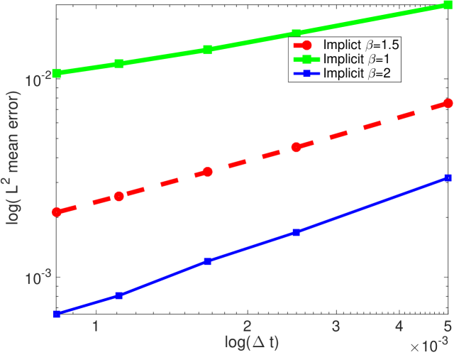
Figure 1: Convergence of the implicit scheme for $\beta=1$, $\beta=1.5$ and $\beta=2$ in (164) for SPDE (162). The orders of convergence in time are $0.47$ for $\beta=1$, $0.72$ for $\beta=1.5$ and $0.93$ for $\beta=2$. The total number of samples used is $100$.

In Figure 1, we can observe the convergence of the the implicit scheme for three noise’s parameters. Indeed, the order of convergence in time is $0.47$ for $\beta=1$, $0.721$ for $\beta=1.5$ and $0.93$ for $\beta=2$. These orders are close to the theoretical orders $0.5$, $0.75$ and $1$ obtained in Theorem 2.3 for $\beta=1$, $\beta=1.5$ and $\beta=2$ respectively.

4.2 Multiplicative noise and application in porous media flow

We consider the following stochastic reactive dominated advection diffusion equation with constant diagonal difussion tensor

$$dX=\left[\left(1+e^{-t}\right)\left(\varDelta X-\nabla\cdot(\mathbf{q}X)\right)-\dfrac{e^{-t}X}{|X|+1}\right]dt+XdW,$$ (170)

with mixed Neumann-Dirichlet boundary conditions on $\Lambda=[0,L_{1}]\times[0,L_{2}]$. The Dirichlet boundary condition is $X=1$ at $\Gamma=\{(x,y):\;x=0\}$ and we use the homogeneous Neumann boundary conditions elsewhere. The eigenfunctions $\{e_{i,j}\}=\{e_{i}^{(1)}\otimes e_{j}^{(2)}\}_{i,j\geq 0}$ of the covariance operator $Q$ are the same as for Laplace operator $-\varDelta$ with homogeneous boundary condition and we also use the noise representation (164). In our simulations, we take $\beta\in\{1.5,2\}$ and $\delta=0.001$. In (14), we take $b(x,u)=u$, $x\in\Lambda$ and $u\in\mathbb{R}$. Therefore, from [19, Section 4] it follows that the operator $B$ defined by (14) fulfills Assumptions 2.4 and 2.5. The function $F$ is given by $F(t,v)=-\dfrac{e^{-t}v}{1+|v|}$, $t\in[0,T]$, $v\in H$ and obviously satisfies Assumption 2.3. The nonlinear operator $A(t)$ is given by

$$A(t)=(1+e^{-t})\left(\varDelta(.)-\nabla.\mathbf{q}(.)\right),\quad t\in[0,T],$$ (171)

where $\mathbf{q}$ is the Darcy velocity obtained as in [24]. Clearly $\mathcal{D}(A(t))=\mathcal{D}(A(0))$, $t\in[0,T]$ and $\mathcal{D}((A(t))^{\alpha})=\mathcal{D}((A(0))^{\alpha})$, $t\in[0,T]$, $0\leq\alpha\leq 1$. The function $q_{i,j}(x,t)$ defined in (12) is given by $q_{i,j}(x,t)=1+e^{-t}$. Since $q_{i,j}(x,t)$ is bounded below by $1+e^{-T}$, it follows that the ellipticity condition (13) holds and therefore as a consequence of Section 2.2, it follows that $A(t)$ is sectorial. Obviously Assumption 2.2 is fulfills.

(a)

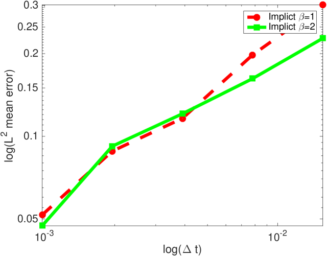
(b)

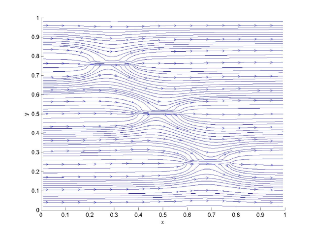
Figure 2: (a) Convergence of the implicit scheme for $\beta=1$, and $\beta=2$ in (164) for SPDE (170). The orders of convergence in time are $0.62$ for $\beta=1$, $0.54$ for $\beta=2$. The total number of samples used is 100. The graph of the streamline $\mathbf{q}$ is given at (b).

In Figure 2, we can observe the convergence of the the implicit scheme for two noise’s parameters. Indeed, the order of convergence in time is $0.62$ for $\beta=1$ and $0.54$ for $\beta=2$. These orders are close to the theoretical orders $0.5$ obtained in Theorem 2.2 for $\beta=1$ and $\beta=2$.

References

- [1] H. Amann, On abstract parabolic fundamental solutions, J. Math. Soc. Jpn. 39 (1987) 93–116.
- [2] S. Blanes, F. Casa, J. A. Oteo, J. Ros, The Magnus expansion and some of its applications, Physics Reports 470 (2009) 151–238.
- [3] S. Blanes, F. Casas, J. A. Oteo, J. Ros, Magnus and Fer expansion for matrix differential equations: the convergence problem, J. Phys. A: Math. Gen. 31 (1998) 259–268.
- [4] S. Blanes, P. C. Moan, Fourth- and sixth-order commutator-free Magnus integrators for linear and non-linear dynamical systems, Appl. Numer. Math. 56 (2006) 1519–1537.
- [5] P. L. Chow, Stochastic partial differential equations, Chapman & Hall/CRC Appl. Math. Nonlinear Sci. ser, 2007.
- [6] P. G. Ciarlet, The finite element method for elliptic problems, Amsterdam: North-Holland, 1978.
- [7] C. M. Elliot, S. Larsson, Error estimates with smooth and nonsmooth data for a finite element method for the Cahn-Hilliard equation, Math. Comput. 58 (1992) 603–630.
- [8] L. C. Evans, Partial Differential Equations, Grad, Stud, 1997.
- [9] H. Fujita, A. Mizutani, On the finite element method for parabolic equation, I; approximation of holomorphic semi-group, J. Math. Soc. Japan 28(4) (1976).
- [10] H. Fujita, T. Suzuki, Evolutions problems (part1). in: P. G. Ciarlet and J. L. Lions(eds.), Handb. Numer. Anal. vol. II, North-Holland, 1991.
- [11] C. González, A. Ostermann, M. Thalhmmer, A second-order Magnus-type integrator for non autonomous parabolic problems, J. Comput. Appl. Math. 189 (2006) 142–156.
- [12] E. Hairer, C. Lubich, G. Wanner, Geometric numerical integration: Structure-preserving algorithms for ordinary differential equations, Springer: Berlin, 2002.
- [13] D. Henry, Geometric Theory of semilinear parabolic equations, Lecture notes in Mathematics, vol. 840, Berlin: Springer, 1981.
- [14] D. Hipp, M. Hochbruck, A. Ostermann, An exponential integrator for non-autonomous parabolic problems, Elect Trans on Numer. Anal. 41 (2014) 497–511.
- [15] M. Hochbruck, C. Lubich, On Magnus integrators for time-dependent Schrödinger equations, SIAM J. Numer. Anal. 41 (2003) 945–963.
- [16] A. Iserles, H. Z. Munthe-Kaas, S. P. Nørsett, A. Zanna A, Lie group methods, Acta Numer. 9 (2000) 215–365.
- [17] A. Jentzen, P. E. Kloeden, G. Winkel, Efficient simulation of nonlinear parabolic SPDEs with additive noise, Ann. Appl. Probab. 21(3) (2011) 908–950.
- [18] A. Jentzen, P. E. Kloeden, Overcoming the order barrier in the numerical approximation of stochastic partial differential equations with additive space-time noise, Proc. R. Soc. A. 465 (2009), 649–667.
- [19] A. Jentzen, M. Röckner, Regularity analysis for stochastic partial differential equations with nonlinear multiplicative trace class noise, J. Differential Equations 252 (2012) 114–136.
- [20] R. Kruse, Optimal error estimates of Galerkin finite element methods for stochastic partial differential equations with multiplicative noise, IMA J. Numer. Anal. 34 (2014) 217–251.
- [21] R. Kruse, S. Larsson, Optimal regularity for semilinear stochastic partial differential equations with multiplicative noise, Electron J. Probab. 65 (2012) 1–19.
- [22] M. Kovács, S. Larsson, F. Lindgren, Strong convergence of the finite element method with truncated noise for semilinear parabolic stochastic equations with additive noise, Numer. Algor. 53 (2010) 309–220.
- [23] S. Larsson, Nonsmooth data error estimates with applications to the study of the long-time behavior of the finite elements solutions of semilinear parabolic problems, Preprint 1992-36, Departement of Mathematics, Chalmers University of Technology (1992)
- [24] G. J. Lord, A. Tambue, Stochastic exponential integrators for the finite element discretization of SPDEs for multiplicative and additive noise, IMA J. Numer. Anal. 2 (2012) 1–29.
- [25] G. J. Lord, A. Tambue, A modified semi-implict Euler-Maruyama scheme for finite element discretization of SPDEs with additive noise, Appl. Math. Comput. 332 (2018) 105–122.
- [26] Y. Y. Lu, A fourth-order Magnus scheme for Helmholtz equation, J. Compt. Appl. Math. 173 (2005) 247–253.
- [27] M. Luskin, R. Rannacher, On the smoothing property of the Galerkin method for parabolic equations, SIAM J. Numer. Anal. 19(1) (1981) 1–21.
- [28] M. Magnus, On the exponential solution of a differential equation for a linear operator, Comm. Pure Appl. Math. 7 (1954) 649–673.
- [29] H. Mingyou, V. Thomée, Some Convergence Estimates for Semidiscrete Type Schemes for Time-Dependent Nonselfadjoint Parabolic Equations, Math. Comp. 37 (1981) 327–346.
- [30] P. C. Moan, J. Niesen, Convergence of the Magnus series, Found. Comput. Math. 8(2008), 291–301.
- [31] J. D. Mukam, A. Tambue, Strong convergence analysis of the stochastic exponential Rosenbrock scheme for the finite element discretization of semilinear SPDEs driven by multiplicative and additive noise, J. Sci. Comput. 74 (2018) 937–978.
- [32] J. D. Mukam, A. Tambue, Magnus-type integrator for the finite element discretization of semilinear non autonomous SPDEs driven by additive noise, Preprint 2018, Available at: https://arxiv.org/abs/1809.06234
- [33] A. Tambue, J. D. Mukam, Convergence analysis of the Magnus-Rosenbrock type method for the finite element discretization of semilinear non autonomous parabolic PDE with nonsmooth initial data, Preprint 2018, Available at: https://arxiv.org/abs/1809.03227
- [34] T. Nambu, Characterization of the Domain of Fractional Powers of a Class of Elliptic Differential Operators with Feedback Boundary Conditions, J. Diff. Eq. 136 (1997) 294–324.
- [35] A. Ostermann, M. Thalhammer, Convergence of the Runge-Kutta methods for nonlinear parabolic equations, Appl. Num. Math. 42 (2002) 367–380.
- [36] A. Pazy, Semigroup of Linear Operators and Applications to Partial Differential Equations, Springer: new York, 1983.
- [37] D. G. Prato, J. Zabczyk, Stochastic equations in infinite dimensions, Encyclopedia of Mathematics and its Applications, Vol. 44, Cambridge: Cambridge University press, 1992.
- [38] C. Prévôt, M. Röckner, A Concise Course on Stochastic Partial Differential Equations, Lecture Notes in Mathematics, Vol. 1905, Springer: Berlin, 2007.
- [39] J. Printems, On the discretization in time of parabolic stochastic partial differential equations, Math. Model. Numer. Anal. 35(6) (2001) 1055–1078.
- [40] R. Seely, Norms and domains of the complex powers , Amer. J. Math. 93 (1971) 299–309.
- [41] J. Seidler, Da Prato-Zabczyk’s maximal inequality revisited I, Math. Bohem. 118(1) (1993) 67–106.
- [42] A. Tambue, J. D. Mukam, Strong convergence of the linear implicit Euler method for the finite element discretization of semilinear SPDEs driven by multiplicative or additive noise, Appl. Math. Comput. 346 (2019) 23–40.
- [43] A. Tambue, J. D. Mukam, Magnus-type integrator for non-autonomous SPDEs driven by multiplicative noise. Discrete Contin. Dyn. Syst. Ser. A. 40(8) (2020), 4597–4624.
- [44] H. Tanabe, Equations of Evolutions, Pitman: London, 1979.
- [45] V. Thomée, Galerkin Finite Element Methods for Parabolic Problems, Springer Series in Computational Mathematics, Vol. 25. Berlin: Springer, 1997.
- [46] X. Wang, Strong convergence rates of the linear implicit Euler method for the finite element discretization of SPDEs with additive noise. IMA J. Numer. Anal. 37(2) (2016) 965–984.
- [47] X. Wang, Q. Ruisheng, A note on an accelerated exponential Euler method for parabolic SPDEs with additive noise, Appl. Math. Lett. 46 (2015) 31–37.
- [48] Y. Yan, Galerkin finite element methods for stochastic parabolic partial differential equations, SIAM J. Num. Anal. 43(4) (2005) 1363–1384.