Harnessing the Power of Serverless Runtimes
for Large-Scale Optimization

Abstract

The event-driven and elastic nature of serverless runtimes makes them a very efficient and cost-effective alternative for scaling up computations. So far, they have mostly been used for stateless, data parallel and ephemeral computations. In this work, we propose using serverless runtimes to solve generic, large-scale optimization problems. Specifically, we build a master-worker setup using AWS Lambda as the source of our workers, implement a parallel optimization algorithm to solve a regularized logistic regression problem, and show that relative speedups up to 256 workers and efficiencies above 70% up to 64 workers can be expected. We also identify possible algorithmic and system-level bottlenecks, propose improvements, and discuss the limitations and challenges in realizing these improvements.

I Introduction

Developments in communication and data storage technologies have made large-scale data collection easier than ever. In order to transform this data into insight or decisions, one often needs to solve a large-scale optimization problem. Examples include optimal classification and regression of data sets, such as, e.g., those available in AWS Public Dataset Program [1], and training of deep neural networks for pattern recognition. Similarly, multi-stage stochastic optimization problems appearing in finance, transportation and energy domains also tend to have larger dimensions than what can be reasonably handled by a single computer.

Traditionally, large-scale problems have been tackled in high-performance computing (HPC) environments. However, HPC environments are expensive and inflexible in the sense that one has to deal with a lot of paperwork to apply for computing power, write programs that obey certain rules and use specific libraries, estimate memory and running-time requirements of these programs and submit them as jobs to the HPC environment accordingly, which are later scheduled by the environment itself. These issues have led to HPC environments’ having limited reach (cf. the discussion in [2]).

Later, with the improvements in virtualization technologies, cloud computing providers started providing dedicated virtual machines (VMs) with different memory and computing power configurations to their customers. Because these dedicated VMs eliminate the burden of paperwork, provide customized programming environments and do not involve job submissions, they have quickly gained wider adoption than HPC environments. However, these solutions still have relatively coarse-grained resource combinations, which might be hard to choose from for a given problem. Even though there exist works such as Ernest [3] and Hemingway [4] that help users choose the correct resource combination for their problems, dedicated VMs are still hard to rescale for new, differently-sized problems. In addition, needing to provision VMs and pay for their idle times are among the reasons that limit VMs’ reach in many scientific applications.

More recently, improvements in container-based solutions have opened an alternative path: serverless runtimes [5, 6, 7]. Serverless runtimes are compute services that let users run their programs in isolated containers without the need for managing or provisioning servers. The main motivation behind the serverless runtimes is, for the providers, that they can simply offer current excess capacity at their backends temporarily to the customers. From the end-user perspective, serverless runtimes are advantageous thanks to their event-driven and elastic nature. Users can not only activate serverless runtimes based on events such as HTTP requests, and thus, only pay for what they use, but also change the resource allocation and number of workers of the runtimes dynamically as needed. Moreover, all major providers support custom programming runtimes, and give away free usage every month. As an example, users get, from each provider, roughly 9 hours of free computing time every month, should they choose to allocate 128 MB memory for their runtimes and spawn 100 workers.

This elasticity of serverless runtimes, however, comes at the expense of some limitations. First, serverless runtimes are stateless. As such, users of serverless runtimes are responsible for keeping track of the states properly in stateful application domains, i.e., when, for instance, running scientific computations or solving optimization problems. Second, serverless runtimes are designed for event-driven, ephemeral applications such as, e.g., manipulating a database record upon an HTTP request, which leads to limited computation times and memory. As a result, careful design of the application code is needed to stay strictly within the bounds, or handle dynamic joining of new workers and leaving of dying workers in long-lived applications. Due to the dynamic nature of the communications, message-passing libraries such as MPI that require static network of nodes are not a viable option, either.

Even though serverless runtimes have been around since the late 2014, the literature involving the serverless runtimes and scientific computations is relatively sparse. There exist studies that examine the task completion latencies [8] and optimize the price of running applications [9] in serverless runtimes. Works such as [10, 11] propose using serverless runtimes to serve (already trained) deep-learning models. However, these applications do not require persistent states or involve frequent communications among workers of the serverless runtimes. In that regard, studies that implement linear algebra primitives [2] and do hyperparameter optimization on neural networks [12] are more relevant examples to using serverless runtimes for stateful and long-lived applications.

In this paper, we try to assess opportunities, limitations and challenges of the serverless runtimes for solving generic, large-scale optimization problems. More specifically,

• We propose using serverless workers for solving optimization problems, collectively, in a distributed way. This is, to the best of our knowledge, the first time serverless runtimes have been used for this purpose. In contrast to the hyperparameter optimization [12], which can be carried out by each worker independently of each other, our work requires that workers share their states at each iteration during the lifetime of the program.

• We show that relative speedups could be expected up to 256 workers and efficiencies above 70% could be expected up to 64 workers, even in a naive implementation.

• We identify possible algorithmic and system-level bottlenecks, propose improvements, and point out the limitations and challenges in implementing the improvements.

The rest of the paper is organized as follows. In Section II, we motivate our work, introduce our experimental setup and list our goals. In Section III, we briefly describe the experiments, and in Section IV, we report our results. Finally, in Section V, we summarize our findings and discuss about possible ways to improve scalability even further.

II Motivation

Figure 1: The external (left) and internal (right) views of the setup. The publisher (PUB) socket broadcasts important signals, such as the termination signal, to the workers and masters.

To evaluate the performance and possible limitations of the serverless runtimes for distributed optimization problems, we choose to focus on the problems of the form

$$\begin{aligned} &\operatorname*{minimize}_{x\in\mathbb{R}^{d}}&&\operatorname{\mathit{\phi}}\left(x\right)\coloneqq\sum_{n=1}^{N}\operatorname{\mathit{f_{n}}}\left(x\right)+\operatorname{\mathit{h}}\left(x\right)\,.\end{aligned}$$ (1)

This loss function $\operatorname{\mathit{\phi}}\left(x\right)$, which appears in many applications, consists of two main parts. The first part is a sum of $N$ smooth functions, $\operatorname{\mathit{f_{n}}}\left(x\right)$, and the second part is a possibly non-smooth function, $\operatorname{\mathit{h}}\left(x\right)$, of the $d$-dimensional decision vector $x$.

Many data-driven machine-learning problems and multi-stage stochastic decision problems can be cast as optimization problems on the form (1). In the case of machine-learning problems, the smooth part encodes the data loss while the non-smooth part is generally used to give preference to a particular solution with desirable properties. For instance, given a data matrix $A$ and a vector $b$, in ridge regression problems, one tries to solve

$$\begin{aligned} &\operatorname*{minimize}_{x\in\mathbb{R}^{d}}&&\sum_{n=1}^{N}\left\lVert\left\langle a_{n},x\right\rangle-b_{n}\right\rVert_{2}^{2}+\frac{\lambda_{2}}{2}\left\lVert x\right\rVert_{2}^{2}\,,\end{aligned}$$

where the first part is the sum of squared residuals coming from ordinary least-squares and the second part is used to prefer solutions with smaller norms. Similarly, in $\ell_{1}$-penalized logistic regression problems, one tries to solve

$$\begin{aligned} &\operatorname*{minimize}_{x\in\mathbb{R}^{d}}&&\sum_{n=1}^{N}\operatorname{log}\left(1+\operatorname{exp}\left(-b_{n}\left\langle a_{n},x\right\rangle\right)\right)+\lambda_{1}\left\lVert x\right\rVert_{1}^{1}\,,\end{aligned}$$

where $b_{n}\in\{-1,1\}$ is the (binary) label for each of the $N$ samples, and the second part in the total loss is used to promote sparse solutions. In the case of multi-stage stochastic optimization problems

$$\begin{aligned} &\operatorname*{minimize}_{x\in\mathbb{R}^{d}}&&\sum_{n=1}^{N}\pi_{n}\operatorname{\mathit{f_{n}}}\left(x\right)+\operatorname{\mathbf{I}}_{\mathbb{X}}\left(Mx\right)\,,\end{aligned}$$

where $\pi_{n}$ denotes the probability of occurring of a scenario in a scenario tree and $\operatorname{\mathbf{I}}_{\mathbb{X}}\left(\cdot\right)$ denotes the indicator function of a set, $\mathbb{X}$, the first part encodes the expected cost of the scenario tree whereas the second part encodes the nonanticipativity of stage variables [13].

One approach to solving problems of the form (1) is to use proximal algorithms [14]. Different proximal algorithms iteratively use the proximal operator

$$x_{k+1} =\operatorname{prox_{\gamma_{k}\operatorname{\mathit{f}}}}\left(x_{k}\right)$$

$$=\arg\,\min_{x}\left\{\operatorname{\mathit{f}}\left(x\right)+\frac{1}{2\gamma_{k}}\left\lVert x-x_{k}\right\rVert_{2}^{2}\right\}$$

for some function $\operatorname{\mathit{f}}\left(\cdot\right)$ and step size $\gamma_{k}$. When the loss function is naturally split into two parts, as in (1), where both parts are closed and proper convex functions, one common approach is to use the alternating direction method of multipliers (ADMM), which, at each iteration $k$, solves the following subproblems [15]:

$$x_{k+1} =\arg\,\min_{x}\left\{\sum_{n=1}^{N}\operatorname{\mathit{f_{n}}}\left(x\right)+\frac{\rho_{k}}{2}\left\lVert x-\left(z_{k}-u_{k}\right)\right\rVert_{2}^{2}\right\}$$ (2)

$$z_{k+1} =\arg\,\min_{z}\left\{\operatorname{\mathit{h}}\left(z\right)+\frac{\rho_{k}}{2}\left\lVert z-\left(x_{k+1}+u_{k}\right)\right\rVert_{2}^{2}\right\}$$ (3)

$$u_{k+1} =u_{k}+x_{k+1}-z_{k+1}\,.$$ (4)

Basically, ADMM iterations alternate between $x$ and $z$-updates by using the proximal operators of the smooth and non-smooth parts of the augmented Lagrangian of the loss function, respectively, and then update the dual variable $u$. Here, $\rho_{k}>0$ is called the penalty parameter.

ADMM is particularly useful when each part of the loss is proximable, i.e., the proximal operator for each part is efficiently obtained, whereas the total sum is not [14]. Moreover, since ADMM handles each part separately, this method is suitable for distributed-memory architectures such as, e.g., the master-worker setups, where worker nodes hold chunks of the smooth loss, and the master node keeps track of the common decision vector and is responsible for handling the non-smooth loss. However, in these setups, one needs to rewrite the ADMM iterations (2)–(4) to obtain the so-called global variable consensus formulation [15]:

$$x_{k+1}^{w} =\arg\,\min_{x}\left\{\sum_{n\in\mathbb{N}_{w}}\operatorname{\mathit{f_{n}}}\left(x\right)+\frac{\rho_{k}}{2}\left\lVert x-\left(z_{k}-u_{k}^{w}\right)\right\rVert_{2}^{2}\right\}\quad\forall w$$ (5)

$$z_{k+1} =\arg\,\min_{z}\left\{\operatorname{\mathit{h}}\left(z\right)+\frac{N\rho_{k}}{2}\left\lVert z-\left(\bar{x}_{k+1}+\bar{u}_{k}\right)\right\rVert_{2}^{2}\right\}$$ (6)

$$u_{k+1}^{w} =u_{k}^{w}+x_{k+1}^{w}-z_{k+1}\quad\forall w\,.$$ (7)

Here, each worker $w$ updates its own copy of $x^{w}$ using its local dataset $\mathbb{N}_{w}$, and the master updates the global variable $z$ using the averaged variables ($\bar{x}$ and $\bar{u}$) of workers.

II-A Setup

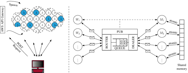
In this paper, we construct a master-worker setup similar to those discussed in [16, 17], and use AWS Lambda as the source of our worker nodes. Currently, AWS Lambda does not allow for inbound network connections. Hence, one cannot obtain a fully connected network of master and worker nodes. For this reason, we build a star network, and assign a local server, i.e., the scheduler, as the central node (see Figure 1). Each node in the star network is connected to the central node with a point-to-point connection. We use ZMQ [18] to handle dynamic joining and leaving of workers in the network, cereal [19] to serialize and deserialize data, and cURL [20] and AWS API Gateway to spawn AWS Lambda functions.

In this setup, the scheduler is responsible for spawning and orchestrating masters and workers. Given a fixed-size problem, the scheduler generates POST requests for the AWS API Gateway to spawn $W$ workers, and embeds the necessary states of the algorithm such as, e.g., problem information and local solver options, inside the requests. It uses ZMQ’s router socket to fair-queue messages coming from the workers. To alleviate the delays in processing the message queue, the scheduler spawns one local master thread per $\bar{W}$ workers, and uses ZMQ’s dealer socket to distribute the messages to the master threads in a round-robin fashion. Master threads process the queue in parallel, average the local variables of the workers using atomic operations, and finally update the global $z$ variable (cf. Equation (6)). If the stopping criterion is satisfied, the scheduler sends a termination signal to the workers and the masters. Otherwise, it broadcasts the new penalty parameter along with the updated $z$ variable to the workers. Pseudocode for the scheduler’s logic is listed in Algorithm 1.

Input: Total number of samples, $N$; problem dimension, $d$; density of non-zero features for each sample, $p$; possibly non-smooth function, $\operatorname{\mathit{h}}\left(\cdot\right)$; number of workers, $W$; maximum number of workers per master, $\bar{W}$; initial penalty parameter, $\rho_{0}$; maximum number of ADMM iterations, $K$; primal residual tolerance, $\epsilon_{r}$; dual residual tolerance, $\epsilon_{s}$; minimum number of local solver iterations, $K_{w}$; gradient norm tolerance, $\epsilon_{g}$; relative function value improvement $\epsilon_{f}$.

1

Output: Optimizer, $x^{\star}$.

2

3foreach $w=1$ to $W$ do API Gateway calls

4       $N_{w}\leftarrow N/W$;

5       spawn($w$; $N_{w}$, $d$, $p$, $\rho_{0}$, $K_{w}$, $\epsilon_{g}$, $\epsilon_{f}$);

6      

7 end foreach

8

9Initialize $k\leftarrow 0$, $t\leftarrow 0$, $\omega\leftarrow 0$, $z_{k}\leftarrow 0$ and $z_{k+1}\leftarrow 0$;

10

11foreach $m=1$ to $\lceil W/\bar{W}\rceil$ do in parallel

12       repeat

13             receive($q_{k}^{w}$, $\omega_{k+1}^{w}$);

             $q\leftarrow q+q_{k}^{w}$;

              // (atomic) reduce

             $\omega\leftarrow\omega+\omega_{k+1}^{w}/N$;

              // (atomic) reduce

14             if All workers have returned then block others

                   // Update the global $z$

15                   $z_{k}\leftarrow z_{k+1}$;

16                   $z_{k+1}\leftarrow\arg\,\min_{z}\left\{\operatorname{\mathit{h}}\left(z\right)+\frac{N\rho_{k}}{2}\left\lVert z-\omega\right\rVert_{2}^{2}\right\}$;

17                   $r\leftarrow\sqrt{q}$;

18                   $s\leftarrow\rho_{k}\left\lVert z_{k+1}-z_{k}\right\rVert_{2}$;

19                   $\rho_{k+1}\leftarrow$ new_penalty($\rho_{k}$, $r$, $s$);

20                   if converged($r$, $s$, $k$; $\epsilon_{r}$, $\epsilon_{s}$, $K$) then

21                         Signal TERM;

22                         $x^{\star}\leftarrow z_{k+1}$;

23                        

24                  else

25                         broadcast($\rho_{k+1}$, $z_{k+1}$);

26                         $q\leftarrow 0$, $\omega\leftarrow 0$, $k\leftarrow k+1$;

27                        

28                   end if

29                  

30             end if

31            

32      until TERM is received;

33 end foreach

34return $x^{\star}$;

Algorithm 1 Scheduler logic.

Worker nodes, on the other hand, load their local problem data and initialize their local solvers based on the state information they receive in the POST requests. Local problem data is not present in the scheduler; instead, the scheduler simply provides enough information so that the workers could either fetch a batch of data samples from hosted datasets or generate the problem data from its closed-form formulation. Then, they update their local primal and dual variables (cf. Equations (5) and (7)) with the penalty parameter and global $z$ variable they receive from the scheduler, and send back the updated ones. We list the pseudocode in Algorithm 2.

Input: $N_{w}$, $d$, $p$, $\rho_{0}$, $K_{w}$, $\epsilon_{g}$, $\epsilon_{f}$.

1

2Load problem data with $N_{w}$, $d$ and $p$ (Section III);

3

4Initialize local solver with $K_{w}$, $\epsilon_{g}$ and $\epsilon_{f}$ (Section III);

5

6Initialize $x_{0}$, $k\leftarrow 0$, $u_{0}\leftarrow 0$ and $z_{0}\leftarrow 0$;

7

8repeat

9       $r_{k}\leftarrow x_{k}-z_{k}$;

10       $u_{k+1}\leftarrow u_{k}+r_{k}$;

11       $x_{k+1}\leftarrow\arg\,\min_{x}\left\{\sum_{n=1}^{N_{w}}\operatorname{\mathit{f_{n}}}\left(x\right)+\frac{\rho_{k}}{2}\left\lVert x-z_{k}+u_{k+1}\right\rVert_{2}^{2}\right\}$;

12       $q_{k}^{w}\leftarrow\left\lVert r_{k}\right\rVert_{2}^{2}$;

13       $\omega_{k+1}^{w}\leftarrow x_{k+1}+u_{k+1}$;

14       send($q_{k}^{w}$, $\omega_{k+1}^{w}$);

15       receive($\rho_{k+1}$, $z_{k+1}$);

16       $k\leftarrow k+1$;

17      

18until TERM is received;

Algorithm 2 Worker logic.

II-B Goals

Our goals in this paper are to assess the performance of serverless runtimes when solving generic optimization problems, and identify possible bottlenecks as well as challenges in addressing them. To this end, we measure the following.

Relative speedup and efficiency. Perhaps the most important measures when evaluating the performance of parallel computations are the relative speedup and efficiency. Relative speedup is the speedup obtained in the new architecture with respect to the old one, i.e., $S_{\text{new}}=t_{\text{old}}/t_{\text{new}}$, where $t_{\text{old}}$ and $t_{\text{new}}$ are the wall-clock times of finishing a task in the old and new architecture, respectively. The efficiency of the new architecture gives an indication of how well the resources are utilized, and is defined as $E_{\text{new}}=S_{\text{new}}/(W_{\text{new}}/W_{\text{old}})$, where $W_{\text{old}}$ and $W_{\text{new}}$ are the number of workers employed in the old and new architecture, respectively.

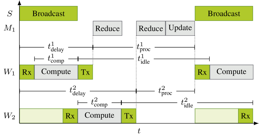
Utilization. To identify bottlenecks in both the algorithm and our experimental setup, we want to understand how the worker functions use their time. To this end, we measure three major utilization metrics: idle time, computation time and delay time of each worker (see Figure 2). The idle time of a worker is measured from the time it sends its local $x$ and $u$ variables until the time it receives the updated $z$ variable from the scheduler. Thus, the idle time includes both the total communication time for the variables and the processing time at the scheduler, i.e., $t^{w}_{\text{idle}}=t^{w}_{\text{comm}}+t^{w}_{\text{proc}}$. The worker’s computation time, $t^{w}_{\text{comp}}$, is the time from when it receives a new global $z$ variable from the scheduler until it returns its updated local variables. Both idle time and computation times are measured by the worker itself. Finally, the delay time associated with a worker as observed from a master is the time between when the scheduler broadcasts the global $z$ variable until the master starts processing the corresponding worker’s $x$ and $u$ updates. The delay time includes both the total communication time and the computation time of the worker, i.e., $t^{w}_{\text{delay}}=t^{w}_{\text{comm}}+t^{w}_{\text{comp}}$. From these metrics, we compute the total communication time of a worker as $t^{w}_{\text{comm}}=t^{w}_{\text{delay}}-t^{w}_{\text{comp}}$. Similarly, we estimate the effect of queuing at the scheduler node by subtracting the delay time from the idle time of the workers, i.e., $t^{w}_{\text{idle}}-t^{w}_{\text{delay}}=t^{w}_{\text{proc}}-t^{w}_{\text{comp}}$. Ideally, processing times at the scheduler should not exceed the workers’ computation times.

Figure 2: Sample timing diagram for the scheduler ($S$), master ($M_{1}$) and workers ($W_{1}$, $W_{2}$) in a 1-master-2-worker setup. “Rx” and “Tx” stand for “reception” and “transmission,” respectively.

Cold starting. Worker functions are not only limited in computation time per invocation but are also stateless. Hence, serverless runtimes suffer from the cold-starting phenomenon, which is defined as the penalty of getting serverless code ready to run [21]. We measure cold-starting times of the workers from the time the scheduler generates the API request until the time the worker contacts the scheduler for the first time. Cold-starting times include transmission of the API request, spawning of the worker and the loading of local data at the worker. Because, in long-lived optimization algorithms, the scheduler needs to spawn new workers to replace those approaching their time limits, cold starting of workers should be small relative to the computation time of the workers.

Responsiveness. The last measure we are interested in assessing is how fast the worker functions respond to the scheduler at each iteration. Because serverless functions are isolated containers that share memory, CPU and network resources with others in the service provider’s backend, their response times can get perturbed by the actual load of the corresponding node in the backend. We would like to understand if there are any stragglers that consistently fall behind the rest.

III Experiments

In our experiments, we follow the procedure outlined in [22] to generate a random instance of $\ell_{1}$-penalized logistic regression problem:

$$\begin{aligned} &\operatorname*{minimize}_{x\in\mathbb{R}^{d}}&&\sum_{n=1}^{N}\operatorname{log}\left(1+\operatorname{exp}\left(-b_{n}\left\langle a_{n},x\right\rangle\right)\right)+\lambda_{1}\left\lVert x\right\rVert_{1}^{1}\end{aligned}$$

with $N=600\,000$ samples, $d=10\,000$ features, $p=0.001$ density (proportion of non-zero features in each sample), and $\lambda_{1}=1$. Every sample has equal probability of having a positive (or negative) label, i.e., $\operatorname{\mathbf{P}}\left[b_{n}=1\right]=\operatorname{\mathbf{P}}\left[b_{n}=-1\right]=0.5$. Indices of the non-zero features for each sample are selected uniformly at random without replacement, whereas the values of non-zero features for samples with positive (or negative) label are drawn independently from a normal distribution $\operatorname{\mathcal{N}}\left(\nu,1\right)$, where $\nu$ is drawn from a uniform distribution on $[0,1]$ (or $[-1,0]$).

For $\ell_{1}$-penalized logistic regression problems, the solution to the subproblem on Line 1 of Algorithm 1 can be obtained easily by applying the soft thresholding operator

$$\operatorname{\mathcal{S}}\left(a;b\right)=\operatorname{max}\left(0,\left(1-b/\left\lvert a\right\rvert\right)\right)a$$

element-wise to $\omega$ with $b=\lambda_{1}/(N\rho_{k})$. However, the subproblem on Line 2 of Algorithm 2 does not have a closed-form solution. Hence, we solve this subproblem (approximately) using an iterative method, FISTA [23] with backtracking. As termination criterion for FISTA, we choose to require that either $\left\lVert g_{\tilde{k}}\right\rVert_{2}\leq\epsilon_{g}=10^{-2}$ or $(f_{\tilde{k}-1}-f_{\tilde{k}})/f_{\tilde{k}-1}\leq\epsilon_{f}=10^{-12}$, where $g_{\tilde{k}}$ and $f_{\tilde{k}}$ are the gradient and function value of the augmented loss at (inner) iteration $\tilde{k}$, respectively. We observe that the gradient norm tolerance and relative function value improvement criteria lead to different number of (inner) iterations for different subproblems, and thus, nonuniform load distributions on the workers. To observe any external effects on the load of workers, we therefore perform two sets of experiments by forcing FISTA to run at least $K_{w}=1$ (nonuniform load) and $K_{w}=50$ iterations (uniform load).

Although problem instances with the aforementioned dimensions can fit in a single AWS Lambda worker with 128 MB of memory, they are too large to handle with $W=1$ or $W=2$ workers within the computation time limit of 15 minutes. As a result, we start with spawning $W=4$ workers and double the number of workers until we do not observe further relative speedup. We consider the ADMM iterations as converged when either both primal and dual residual norms are small enough, i.e., $r\leq\epsilon_{r}=2\cdot 10^{-2}$ and $s\leq\epsilon_{s}=2\cdot 10^{-2}$, or $K=100$ iterations have passed. Finally, we use the following rule [15] to adjust the new penalty parameter at each iteration:

$$\rho_{k+1}=\begin{cases}2\rho_{k}&\text{if }r>10s\,,\\ 0.5\rho_{k}&\text{if }s>10r\,,\\ \rho_{k}&\text{otherwise,}\end{cases}$$

starting with $\rho_{0}=1$.

IV Results

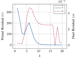
In our experiments, we observe speedups in wall-clock times of ADMM iterations up to $W=256$ workers. In all the experiments, we observe that ADMM iterations converge within at most $K=23$ iterations by satisfying the primal and dual residual tolerance values. In Figure 3, we provide traces of the residuals for $W=64$ workers when the workers had nonuniform load distributions.

Figure 3: Convergence of the residuals for $W=64$ workers and $K_{w}=1$.

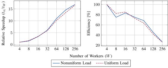
Relative speedup and efficiency. Because our problem instances cannot be solved by fewer than four workers, we report relative speedup and efficiency metrics with respect to $W=4$. In Figure 4, we observe that relative speedups up to 17 times can be expected in both uniform and nonuniform load scenarios, which translates to 26% efficiency.

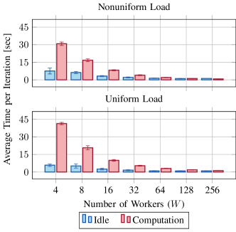
We also observe that there is a sharp decrease in efficiency when going from $W=64$ (74%) to $W=256$ (26%) workers. This is best explained in Figure 5, which shows the average idle and computation times per iteration. As can be seen, after $W=64$ workers, average idle time starts beating average computation time. Basically, when we increase the number of workers, average computation time constantly decreases. On the contrary, average idle time decreases up to a point and then increases again with increasing number of workers. The reason is that increasing the number of workers improves the worst-case solution times of subproblems (which get smaller as the number of workers increases), which in turn improves the idle time up to the level set by transmission time of the decision vector. After this level, queuing effects take over with increasing number of workers. In the ideal case, instead of fixing the problem size and increasing the number of workers, one should aim at increasing both the problem size and the number of workers to benefit from more computing power, which is in line with Gustafson’s Law [24].

The main difference between uniform and nonuniform loads is that the average computation times are increased per iteration and the variance in both idle and computation times is decreased for uniform loads. This is because we make the local solvers run for roughly the same number of iterations ($K_{w}=50$).

Figure 4: Speedup and effiency plots. Speedup and efficiency of the algorithm are reported relative to $W=4$ workers, since fewer workers are not sufficient to solve the problem within the time limit.

Figure 5: Average utilization of Lambda workers. Time spent in idle and computation is first averaged over total number of iterations, and then over total number of Lambda functions. Error bars show one standard deviation among the workers.

Utilization. Even though AWS Lambda does not guarantee any performance measures other than the built-in fault tolerance and allocation of CPU power, network bandwidth and disk input/output proportional to the selected memory size of the workers, we have observed consistent behavior in workers’ performance during our experiments (see Figure 6 for a sample histogram for $W=64$ workers).

Figure 6: Utilization histograms for Lambda workers when $W=64$ workers are used.

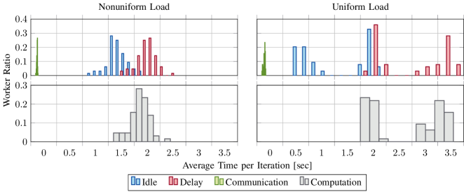
As expected, nonuniform loads (Figure 6, left) result in computation time distributions centered around a smaller mean and with a more peaked shape compared to those of the uniform loads (Figure 6, right). Because the delay time is dominated by the computation time of workers in our experiments (cf. communication time in Figure 6), it also has a similar behavior in its distribution. On the contrary, because the idle time is a measure of the discrepancy between the fastest and slowest workers for a fixed problem size and master-worker setup, it is decreased with uniform loads. As a result, uniform loads result in less queuing times for workers. For instance, as can be seen in Figure 7, when we have $W=256$ workers, workers with uniform loads still spend more time in computing than idling, whereas those with nonuniform loads idle more. Unfortunately, having workers spend more time computing than idling does not directly translate to a more efficient algorithm, as ADMM iterations can sill converge to modest accuracies with inexact $x$-minimization steps [15].

Figure 7: Utilization histograms for Lambda workers when $W=256$ workers are used.

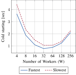
Cold starting. When generating AWS API Gateway requests, we use cURL’s multi interface that enables multiple simultaneous transfers in the same (background) thread. We report cold-starting times of AWS workers in Figure 8, which is representative of spawning new workers in bulks with problem data that has closed form representations. In the experiments, we observe that the cold starting of workers are rather consistent, and, up to $W=64$ workers, well below the average time spent in computation per single ADMM iteration. Afterwards, the cold starting degrades due to the queuing of bulk requests in the (background) thread.

Figure 8: Cold starting of Lambda workers. The plot shows the first response time of the fastest and slowest workers after getting spawned.

Responsiveness. Finally, we compute the fraction of iterations in which each worker is among the slowest 10% to return its local solutions to the scheduler, and plot the corresponding histogram in Figure 9. Similar to the utilization metrics, workers have consistent responsiveness. There are not any stragglers which fall behind more than one third of the total iterations, and, only a very few of the workers lag behind more than one forth of the total time. Moreover, the fastest group, i.e., the 0-bin in Figure 9, has a bigger set of workers in uniform load scenario compared to that in the nonuniform load.

Figure 9: Responsiveness of Lambda workers during the algorithm when $W=64$ workers are used.

V Conclusion

In this work, we have investigated the performance and limitations of serverless runtimes when solving generic, distributed optimization problems. To this end, we have built a master-worker setup in a star network, in which the central node is a managed multi-core server and the other nodes are AWS Lambda functions. In our experiments, we have used synchronous parallel ADMM iterations to solve regularized logistic regression problems, and observed relative speedups up to 256 workers and efficiencies above 70% up to 64 workers. Furthermore, even though AWS Lambda does not give any specific performance guarantees, the workers have satisfactory cold-starting times compared to their computation times and they do not show major straggling problems that could hinder the performance of the algorithms.

Because serverless runtimes are stateless and have limited compute times, they have a major limitation when solving optimization problems. For long-lived optimization algorithms, serverless runtimes require careful bookkeeping of algorithm states as well as fault tolerance of workers approaching their time limits. Second, inability to have inbound network connections at serverless runtimes makes it impossible to use collective communication patterns such as, e.g., MPI’s AllReduce or Bcast, among the nodes.

V-A Outlook and Future Work

Despite their aforementioned limitations, we believe that serverless runtimes, with their availability and elasticity, are promising candidates for scaling the performance of distributed optimization algorithms. There are some possible algorithmic and system-level improvements to obtain better efficiencies, which are left as future work.

Algorithmic improvements. In this work, we have considered a single family of algorithms, i.e., synchronous parallel ADMM. We have observed that increasing the computation times of worker nodes by making them use more iterations in their local solvers does not directly translate to improved efficiencies. One way to improve the parallel efficiency is to try asynchronous parallel ADMM [25, 26, 27] or other (asynchronous) families of algorithms that could potentially allow for better scalability. An alternative approach could be to account for the slowest workers at each iteration in the synchronized setting. In the machine learning community, there have been recent works [3, 28, 29] that simply discard a small percentage of the slowest workers in synchronized parallel algorithms. In these works, discarding information contained within the slowest workers’ messages acts as an implicit regularization, and the authors obtain not only improved timings but also better classification performance. However, for generic optimization problems, this approach will result in a suboptimal solution. Instead, one can try coded optimization techniques [30, 31, 32] to alleviate the straggler effects in the synchronized setting.

System-level improvements. In our experiments, we have solved problems that involve decision vectors of size $d=10\,000$. Broadcasting this vector using point-to-point communications to workers, and reducing the information coming from workers collectively using multiple masters have negligible effect during computations (cf. communication and computation times in Figure 6). However, for decision vectors with sizes larger than, e.g., $d=80\,000$, the communication time will be on par with the computation time. In these cases, spawning masters as serverless runtimes and using the ideas in [2] to replace the shared memory of the masters with the high-bandwidth, high-latency distributed object store could be beneficial in improving the communication times.

References

- [1] Amazon Web Services. (2019, Jan.) AWS Public Dataset Program. [Online]. Available: https://aws.amazon.com/opendata/public-datasets/
- [2] V. Shankar, K. Krauth, Q. Pu, E. Jonas, S. Venkataraman, I. Stoica, B. Recht, and J. Ragan-Kelley, “numpywren: serverless linear algebra,” Oct. 2018. [Online]. Available: http://arxiv.org/abs/1810.09679v1
- [3] S. Venkataraman, Z. Yang, M. Franklin, B. Recht, and I. Stoica, “Ernest: Efficient performance prediction for large-scale advanced analytics,” in 13th USENIX Symposium on Networked Systems Design and Implementation (NSDI 16). Santa Clara, CA: USENIX Association, 2016, pp. 363–378. [Online]. Available: https://www.usenix.org/conference/nsdi16/technical-sessions/presentation/venkataraman
- [4] X. Pan, S. Venkataraman, Z. Tai, and J. Gonzalez, “Hemingway: Modeling distributed optimization algorithms,” Feb. 2017. [Online]. Available: http://arxiv.org/abs/1702.05865v1
- [5] Amazon Web Services. (2018, Dec.) AWS Lambda — Serverless Compute. [Online]. Available: https://aws.amazon.com/lambda/
- [6] Microsoft Azure. (2018, Dec.) Azure Functions — Serverless Architecture. [Online]. Available: https://azure.microsoft.com/en-us/services/functions/
- [7] Amazon Web Services. (2018, Dec.) Cloud Functions — Event-driven Serverless Computing. [Online]. Available: https://cloud.google.com/functions/
- [8] M. Gorlatova, H. Inaltekin, and M. Chiang, “Characterizing task completion latencies in fog computing,” Nov. 2018. [Online]. Available: http://arxiv.org/abs/1811.02638v1
- [9] T. Elgamal, A. Sandur, K. Nahrstedt, and G. Agha, “Costless: Optimizing cost of serverless computing through function fusion and placement,” Nov. 2018. [Online]. Available: http://arxiv.org/abs/1811.09721v1
- [10] V. Ishakian, V. Muthusamy, and A. Slominski, “Serving deep learning models in a serverless platform,” Oct. 2017. [Online]. Available: http://arxiv.org/abs/1710.08460v2
- [11] Google Cloud. (2018, Dec.) Solutions — Building a Serverless Machine Learning Model. [Online]. Available: https://cloud.google.com/solutions/building-a-serverless-ml-model
- [12] L. Feng, P. Kudva, D. D. Silva, and J. Hu, “Exploring serverless computing for neural network training,” in 2018 IEEE 11th International Conference on Cloud Computing (CLOUD). IEEE, Jul. 2018.
- [13] J. Eckstein, J.-P. Watson, and D. L. Woodruff, “Asynchronous projective hedging for stochastic programming,” Oct. 2018. [Online]. Available: http://www.optimization-online.org/DB_HTML/2018/10/6895.html
- [14] N. Parikh, “Proximal algorithms,” Foundations and Trends® in Optimization, vol. 1, no. 3, pp. 127–239, 2014.
- [15] S. Boyd, “Distributed optimization and statistical learning via the alternating direction method of multipliers,” Foundations and Trends® in Machine Learning, vol. 3, no. 1, pp. 1–122, 2010.
- [16] M. Li, L. Zhou, Z. Yang, A. Li, F. Xia, D. Andersen, and A. J. Smola, “Parameter Server for distributed machine learning,” in Big Learning Workshop, Advances in Neural Information Processing Systems 26 (NIPS), 2013.
- [17] L. Xiao, A. W. Yu, Q. Lin, and W. Chen, “Dscovr: Randomized primal-dual block coordinate algorithms for asynchronous distributed optimization,” Oct. 2017. [Online]. Available: 1710.05080v1
- [18] MQ. (2017) Distributed Messaging. [Online]. Available: http://zeromq.org/
- [19] USCiLab. (2018, Aug.) cereal. [Online]. Available: https://uscilab.github.io/cereal/
- [20] (2018, Aug.) curl. [Online]. Available: https://curl.haxx.se/
- [21] I. Baldini, P. Castro, K. Chang, P. Cheng, S. Fink, V. Ishakian, N. Mitchell, V. Muthusamy, R. Rabbah, A. Slominski, and P. Suter, Serverless Computing: Current Trends and Open Problems. Singapore: Springer Singapore, 2017, pp. 1–20.
- [22] K. Koh, S.-J. Kim, and S. Boyd, “An interior-point method for large-scale -regularized logistic regression,” Journal of Machine Learning Research (JMLR), vol. 8, pp. 1519–1555, 2007. [Online]. Available: http://www.jmlr.org/papers/volume8/koh07a/koh07a.pdf
- [23] A. Beck and M. Teboulle, “A fast iterative shrinkage-thresholding algorithm for linear inverse problems,” SIAM Journal on Imaging Sciences, vol. 2, no. 1, pp. 183–202, Jan. 2009.
- [24] J. L. Gustafson, “Reevaluating amdahl’s law,” Communications of the ACM, vol. 31, no. 5, pp. 532–533, May 1988.
- [25] R. Zhang and J. Kwok, “Asynchronous distributed ADMM for consensus optimization,” in Proceedings of the 31st International Conference on Machine Learning (ICML). JMLR.org, 2014, pp. 1701–1709. [Online]. Available: http://jmlr.org/proceedings/papers/v32/zhange14.pdf
- [26] T.-H. Chang, M. Hong, W.-C. Liao, and X. Wang, “Asynchronous distributed ADMM for large-scale optimization—part i: Algorithm and convergence analysis,” IEEE Transactions on Signal Processing, vol. 64, no. 12, pp. 3118–3130, Jun. 2016.
- [27] T.-H. Chang, W.-C. Liao, M. Hong, and X. Wang, “Asynchronous distributed ADMM for large-scale optimization—part II: Linear convergence analysis and numerical performance,” IEEE Transactions on Signal Processing, vol. 64, no. 12, pp. 3131–3144, Jun. 2016.
- [28] J. Chen, X. Pan, R. Monga, S. Bengio, and R. Jozefowicz, “Revisiting distributed synchronous sgd,” Apr. 2016. [Online]. Available: http://arxiv.org/abs/1604.00981v3
- [29] M. Teng and F. Wood, “Bayesian distributed stochastic gradient descent,” in Advances in Neural Information Processing Systems 31 (NIPS). Curran Associates, Inc., 2018, pp. 6380–6390. [Online]. Available: http://papers.nips.cc/paper/7874-bayesian-distributed-stochastic-gradient-descent.pdf
- [30] R. Tandon, Q. Lei, A. G. Dimakis, and N. Karampatziakis, “Gradient coding: Avoiding stragglers in distributed learning,” in Proceedings of the 34th International Conference on Machine Learning, ser. Proceedings of Machine Learning Research, vol. 70. PMLR, Aug. 2017, pp. 3368–3376. [Online]. Available: http://proceedings.mlr.press/v70/tandon17a.html
- [31] C. Karakus, Y. Sun, S. Diggavi, and W. Yin, “Straggler mitigation in distributed optimization through data encoding,” in Advances in Neural Information Processing Systems 30 (NIPS). Curran Associates, Inc., 2017, pp. 5434–5442. [Online]. Available: http://papers.nips.cc/paper/7127-straggler-mitigation-in-distributed-optimization-through-data-encoding.pdf
- [32] J. Zhu, Y. Pu, V. Gupta, C. Tomlin, and K. Ramchandran, “A sequential approximation framework for coded distributed optimization,” Oct. 2017. [Online]. Available: http://arxiv.org/abs/1710.09001v1