Quantum simulation dynamics and circuit synthesis of FMO complex on an NMR quantum computer
Abstract
Recently, the dynamics simulation of light-harvesting complexes as an open quantum system, in the weak and strong coupling regimes, has received much attention. In this paper, we investigate a digital quantum simulation approach of the Fenna-Matthews-Olson (FMO) photosynthetic pigment-protein complex surrounded with a Markovian bath, i.e., memoryless, based on a nuclear magnetic resonance (NMR) quantum computer. For this purpose, we apply the decoupling(recoupling) method, which is turn off(on) the couplings and also Solovay-Kitaev techniques to decompose Hamiltonian and Lindbladians into efficient elementary gates on an NMR simulator. Finally, we design the quantum circuits for the unitary and non-unitary part due to the system-environment interactions of the open system dynamics.
Keywords Quantum simulation, FMO complex, NMR quantum computation.
1 Introduction
Real quantum systems interact as open systems with their surroundings, and understanding the dynamics of the interacting system, including many degrees of freedom in an environment, is one of the significant challenges in physics, chemistry, and biology. Dynamic evolution of open systems treatment due to the decoherence, and dissipation effects isn’t unitary and It’s very complicated and often used to describe the dynamics of proximity like the Born-Markov approximation [1]. Due to the exponential growth of variables, efficiently simulating quantum systems with complex many-body interactions are hard for classical computers. For this reason, the idea of modeling a quantum computer to simulate large quantum systems was initially been suggested, by R. Feynman [2], where he conjectured that the quantum computers might be able to carry the simulation more efficiently than the classical one. Although, implementation of universal quantum computers for large sizes of open systems are not available yet. According to this, a quantum simulation was proposed to solve such an exponential explosion problem using a controllable quantum system [2], and typically classified into two main categories, namely, analogs that are more scalable [3] and digital that are more flexible and universal [4] . A lot of analytical and numerical methods had been employed to simulate the dynamics of open quantum systems [5, 6, 7, 8, 9, 10]. Different platforms have been used for implementing quantum simulators, such as ions trapped in the optical cavity [11, 12], cold atoms in optical lattices [13], super-conducting qubits [14, 15], photons [16], quantum dots [17] and the spin qubits based on magnetic resonance process [18, 19, 20, 21, 22]. We will consider quantum simulation dynamics of photosynthetic light-harvesting complexes as an open system in terms of some time sequence quantum gates. In all of the photosynthetic organisms, light is absorbed by pigments such as chlorophyll and carotene in antenna complexes, and then this energy transfers as an electronic excitation to a reaction center where charge separation occurs through the processes. The FMO complex is made of three identical monomers where each monomer involves seven bacteriochlorophyll molecules surrounded by a protein environment. Neill Lambert et al. [23] introduced interesting progress in quantum biology, where they performed an experimental and theoretical studies on the photosynthesis such as the quantum coherent energy transport, entanglement, and tests of quantumness. Decoherence in biological systems are being studied in Ref. [24] and principles of a noise-assisted transport as well as the origin of long-lived coherences for the FMO complex in photosynthesis was given. The exciton-energy transfer in light-harvesting complexes has been investigated by various methods such as the Forster theory in a weak molecular interaction limit or by the Redfield master equations derived from Markov approximation in a weak coupling regime between molecules and environment [25, 26, 27, 28, 29, 30]. In general, the dynamics of an open quantum system can be divided into two categories. Markovian and non-Markovian dynamics that depend on the strength of the coupling between the system and the environment. In the weak coupling regime between the system and the environment, often proximity like the Born and Markov approximations are used. Non-Markovian effects on energy transfer dynamic are significant [31, 32]. Here, we ignore the non-Markovian effects and the exact dynamics of the FMO complex can be described with the Markovian Lindblad master equation, which we will discuss in this article. It should be noticed that effective dynamics of the FMO complex is modeled by a Hamiltonian which describes the coherent exchange of excitations among different sites, also local Lindblad terms that take into account the dissipation and dephasing processes caused by a surrounding environment[33, 34]. In the one hand, simulations of the light-harvesting complexes have considered, and a large number of various experimental and analytical studies have been done. For instance, numerical analysis of a spectral density based on the molecular dynamics has been studied in Refs. [32, 35, 36], as well as the corresponding dynamics had been investigated based on a two-dimensional electronic spectroscopy [37], superconducting qubits [38] and numerically and analytically simulations [39, 40]. On the other hand, nuclear spin systems are good candidates for a quantum simulator, because they include long coherence times and may be manipulated by complex sequences of radio frequency (RF) pulses, then they can be carried out easily using modern spectrometers. Because of the importance of the subject, we present an effective nuclear spin system using an NMR-based quantum simulator as a controllable quantum system that can be applied to simulate the Hamiltonian and Lindbladians of the FMO complex. We investigate a scheme based on the recoupling and decoupling methods [41] ,which are particularly relevant to the connection of any two nuclear spins using RF pulses in any selected time for simulating the Hamiltonian of FMO complex. Here, we assume the Solovay-Kitaev decomposition strategy for single-qubit channels [10] to simulate the non-unitary part of quantum master equation and circuits obtained on the NMR quantum computation.
The paper is organized as follows. In Sec. 2, the FMO complex will be introduced. In Sec. 3, simulation of Hamiltonian of the FMO complex by an NMR simulator is expressed. In Sec. 4, corresponding calculations to simulate the non-unitary part will be given. Finally, Sec. 5 is devoted to some conclusions.
2 FMO complex
The FMO complex is generally constituted of multiple chromophores which transform photons into exactions and transport to a reaction center. The exciton dynamics for the light-harvesting system (e.g., in the FMO complex) is modelled by a Markovian master equation of the form
| (1) |
which contains the coherent exchange of excitation and local Lindblad terms [33, 34]. The quantum coherent evolution is governed by a electronic tight-binding Hamiltonian with seven bacteriochlorophyll (BChl) sites in general form:
| (2) |
where are the site energies and is the Coulomb couplings of the transition densities of the chromophores, often taken to be of the (Forster) dipole-dipole form. We consider one excited molecule in time and others in ground states in every cycle so it goes as seven bacteriochorophyll sites space that are the basis denoting the excitations at site i for . To facilitate the comparison with NMR quantum computing, we rewrite the total Hamiltonian Eq.2 using Pauli matrices
| (3) |
where is single-qubit Hamiltonian and is long-term interaction. For expressing the dynamics of non-unitary part, we assume that the system affected by two distinct types of noise are called the dissipative and dephasing processes. Dissipative effect passes the excitation energy with rate to the environment and dephasing process destroys the phase coherence with the rate of the site . Both of these processes can be describe using a Markovian master equation with local dephasing and dissipation terms. For the FMO complex in the Markovian master equation approach, the dissipative and the dephasing processes are captured, respectively, by the Lindblad super-operators as follows
| (4) |
| (5) |
Finally, the total transfer of excitation is measured by the population in the sink. In the next section, we introduce the recoupling and decoupling method attached to simulate the Hamiltonian of the FMO complex.
3 Simulation of Hamiltonian with recoupling and decoupling method
We use, the recoupling, and decoupling method with Hadamard matrix’s approach to simulate the Hamiltonian of FMO complex and perform a specific coupling in the NMR quantum computation. The task of turning-off all the couplings is known as decoupling, and also doing this for a selected subset of couplings is known as recoupling. These pulses are single-qubit operations that transfer Hamiltonian in time between two pulses so that unwanted couplings in a consecutive evolution cancel each other. The decoupling part must be chosen as the Hadamard matrices , where we have used instead of the positive and negative sign, respectively. We use the gates to control the signs of for each spin over an equal interval, and we will achieve sign matrix , where each column represents a time interval and each row indicates a qubit; for details, see Ref. [41]. When does not necessarily exist, we start with and finally take . Similarly, for the recoupling part, we use a normalized Hadamard matrix , which has only ’s in the first row and column. Then, to implement selective recoupling between the and qubit, we exclude the first row and taking the second row of to be the and qubit row of , also the other rows of can be chosen from the remaining rows of .
When a nuclear spin is placed in a static magnetic fieldalong the z-direction, the dynamical evolution will be dominated by the internal Hamiltonian , where is the nuclear gyromagnetic ratio, is the chemical shift arising from the partial shielding of by the electron cloud surrounding the nuclear spin, and is the Larmor frequency. Note, is the angular momentum operator related to Pauli matrix . For multiple-spin systems, heteronuclear spins are easily distinguished due to the distinct and thus very different in the magnitude of hundreds of MHz, while homonuclear spins are often individually addressed by the distinct due to different local environments. Furthermore, the qubit-qubit interactions are the natural mediated spin-spin interactions called Hamiltonian J-coupling terms. The Hamiltonian for nearest-neighbor interaction is . Therefore, the total Hamiltonian for a N-spin system is
| (6) |
which forms a well-defined multi-qubit system used in most NMR quantum computing [42].
The Hamiltonian called Longitudinal Ising model in solid-state systems and denotes a coupling strength between the and qubits. This Hamiltonian evolved in time by the following unitary operator
| (7) |
The key insight of this paper is that to use the NMR quantum simulator with to simulate the Hamiltonian of Eq.3 in two steps: the first step is to simulate single-qubit Hamiltonian and the second one is to simulate interaction part . We then combine and to obtain the complete Hamiltonian of Eq.3. The detailed description of these steps is as given below.
3.1 Simulation of
It is clear that the Hamiltonian of the FMO complex includes seven-qubits, then the sign matrix should have seven rows. On the other hand, the Hadamard matrix of order-7 does not exist; then we consider a Hadamard matrix of order-8 to obtain a sign matrix . We obtain the time evolution for the first qubit and generalize it to seven qubits, for this purpose by using the Eq.(7), and removing the last row of :
| (8) |
a possible sign matrix can be obtained as follows
| (9) |
In continuation with the following pulse sequence
using the Eq.(7) and the Paul matrices, we have
| (10) |
which provides a time evolution of the first qubit, i.e.
| (11) |
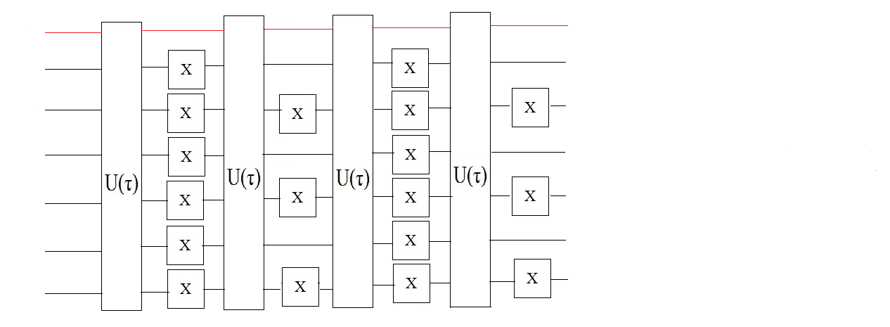
Quantum circuits to simulate is shown in Figure 1. Similarly, for seven qubits it can be written as
| (12) |
with
| (13) |
where , with , and prime denotes that if is odd (even) number, is considered as a even (odd) number. Then, the time evolution of obtain at = . To test our quantum circuit, we use the Forest (pyQuil) software platform. It is an open-source Python library developed by Rigetti for constructing, analyzing, and running quantum programs [43]. We consider the initial state as , and then putting , implement our circuit. The output of circuit on Forest is
which matches the theory, i.e. is equivalent to . Since the time evolution occurred only on the first qubit, it means that the recoupling has done( See Appendix I for details and code).
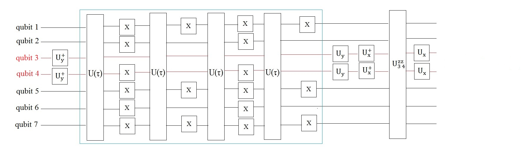
3.2 Simulation of
In this subsection, we simulate a time evolution of the Hamiltonian , by using a decoupling method. Similar to the case already discussed in the previous section, the sign matrix is obtained by a Hadamard matrix . We implement recoupling between the and qubits and finally expressed in the general case for seven qubits. Firstly, we exclude the first row of and take the second row of to be the and qubit row of , Finally, five other rows of can be chosen from the remaining rows of . A possible structure is
| (14) |
in this case, the pulse sequence can be written as
Along with the identity , it can be recast into:
| (15) |
Note we consider and interaction for two nearest-neighbor-interacting qubits, and then by using the single-qubit operations, we obtain:
| (16) |
where we have used the notation . Also, for seven qubits it can
be written, generally, as follows
where , with and considering . Quantum circuits to simulate is shown in figure 2. Similar to the previous
one, by implementing circuit on the Forest’s software
platform by:
it is approximately equal with direct calculation of . It is easily seen that coupling between the and site is conserved, i.e. the decoupling yield with high efficiency. With all nearest-neighbor coupling operators and being simulated, one can extend them to the long-range interactions in a straightforward manner. Since, both the Hamiltonian and are available, then the total Hamiltonian can be obtained by the Trotters formula [44]:
| (17) |
Here we have used as a Hamiltonian simulator, which can be used instead of other Hamiltonian such as the transverse Ising model, the and Heisenberg model.
4 Quantum simulation of the non-unitary part
It can be deduced from the non-unitary part of the FMO complex that each monomer has seven bacteria and considered as a system of seven qubits. We consider one of them which interacts with their surroundings and study its dynamics with the single-qubit channels approach. So we restrict ourselves to single-qubit states and begin by recalling some geometric properties of them [45]. In general, every density matrix can be written in terms of the standard bases, , as with and =. Each single qubit quantum channel can then be represented in this basis by a unique matrix , where is a matrix and , denote row and column vectors respectively. The density matrix through the action of a channel will change as follows.
| (18) |
with and the channel, , is considered as an affine map, i.e.
| (19) |
by
| (20) |
Also, the matrix can be rewritten in the following form
| (21) |
in this case, the Kraus operators will be given by
| (22) |
| (23) |
where and . For one qubit state the Eq. (4) becomes
| (24) |
by using the damping basis methods [46, 47] (details are given in the Appendix) and considering
one can find as the following equation
| (25) |
Any single-qubit channel (CPTP map) can be simulated with one ancillary qubit, one CNOT, and four single-qubit operations[10]. The two rotation operations are applied to cover the Kraus operator’s action, and another single-qubit operation is used only to diagonalize the matrix . We want to design a circuit to simulate the non-unitary part dynamics of the FMO complex on the NMR computer. So recalling some properties of the NMR quantum computation [48], we shall consider a physical system which consists of a solution of identical molecules. Each molecule has N magnetically inequivalent nuclear spins, which serve as qubits. Nuclear spins interact via a dipole-dipole coupling or indirect coupling mediated by electrons. In any case, in the presence of a strong external magnetic field, only the secular parts are important [41]. Single qubit operations can be induced by the RF magnetic fields, oriented in the plane perpendicular to the static field. The RF pulse can be selectively addressed spin by an oscillator at angular frequency . The general form of single-qubit gates in quantum information processing may become as the RF pulse along the -axis induces the rotation operator where is proportional to the pulse duration (pulse width) and amplitude. For example can be considered as a single pulse around -axes, then the Hadamard gate can create a -pulse around -axes followed by a -pulse around -axes, too. Coupled logic gates can be naturally performed by a time evolution of the system. It can be assumed that the individual coupling term can be selectively turned on to perform a coupled operation between and qubits, next turning on the coupling term for time , leads to the evolution of logic gate . Together with setting all of single-qubit transformations, the fulfills a requirement for universality. Returning to the original problem and starting by the following assumptions:
the kraus operators are obtained as follows
| (26) |
| (27) |
As mentioned above an action of the Kraus operators can be represented through the rotations = with and in a quantum circuit. For implementing the rotations and , respectively, we set
| (28) |
and
| (29) |
Along with the CNOT gate and above mentioned preliminaries, we can obtain a quantum circuit for implementation of the quantum channel of T for dissipation process that shown in Figure. 3. For the dephasing process, a straightforward calculations of the Kraus operators leads to
| (30) |
| (31) |
similarly, this process is also implemented based on the NMR simulator. In comparing with the implementation process of the and we choose here and and and respectively.
\Qcircuit@C=0.6em @R=1.95em \lstick|q_sys⟩
& \gateU(δ) \gateR_z(π2) \qw \qw \multigate1cZ \qw \qw \qw \gateX \gateU(φ) \qw \qw
\lstick|q_anc⟩ \qw \gateR_y(2γ_1) \gateH \gateR_z((π2) \qw \ghostcZ \qw \gateH \qw \gateR_y(2γ_2) \meter \qw \qw
5 Conclusion
In this paper, we investigated a quantum simulation of the
FMO complex dynamics by nuclear spin systems. We employed recoupling
and decoupling methods to simulate the Hamiltonian of FMO complex,
then for quantum simulation of the non-unitary part dynamics of FMO
complex with the single-qubit channel’s a quantum circuit had obtained.
Finally, the obtained circuit implements an NMR quantum computation
based on Forest’s software platform (pyQuil). The output of
the pyQuil code is compatible with direct calculation, too. Also,
dynamical simulation of the FMO complex optimized with currently
available technology. However, we will study the non-Markovian dynamics of the FMO complex base on NMR quantum computation in the future.
Appendix I
As mentioned above pyQuil is an open-source Python library developed by Rigetti for constructing, analyzing, and running quantum programs. It is built on top of Quil, an open quantum instruction language (or simply quantum language), designed specifically for near-term quantum computers and based on a shared classical/quantum memory model [43]. By using this instruction we implement the Eq.(10) on pyQuil by below code:
from pyquil.quil import
from pyquil.api import WavefunctionSimulator
for i in list1:
p+=H(i),CPHASE(np.pi,i+1,i),RX(0.25,i),CPHASE(np.pi,i+1,i),H(i),RZ(0.25,i)
for i in list1:
if i>0:
p+=X(i)
p+=X(2),X(4),X(6)
for i in list1:
p+=H(i),CPHASE(np.pi,i+1,i),RX(0.25,i),CPHASE(np.pi,i+1,i),H(i),RZ(0.25,i)
for i in list1:
if i>0:
p+=X(i)
for i in list1:
p+=H(i),CPHASE(np.pi,i+1,i),RX(0.25,i),CPHASE(np.pi,i+1,i),H(i),RZ(0.25,i)
p+=X(2),X(4),X(6)
#
#
#
#
Similarly, the code to implement of Ee.(16) can be written straightforward.
Appendix II
To solve the master equation which is the generator of a semigroup of a quantum channel at first, we must find left and right eigen-operators and which satisfying the following condition:
| (32) |
| (33) |
By using the left action of superopertor that defined as for arbitrary Hermitian operator and any density matrix can find that = and where Tr refers to the usual trace, so that initial state writing in damping base method such [46, 47]
| (34) |
and
| (35) |
where . So for solving equation (23) we utilize these set {, , and } as right eigen-operators, we obtain:
| (36) |
| (37) |
| (38) |
| (39) |
For left eigen-operators action we consider an appropriate set of operators { , , and }
| (40) |
| (41) |
| (42) |
| (43) |
References
- [1] H.-P. Breuer, F. Petruccione, et al., The theory of open quantum systems. Oxford University Press on Demand, 2002.
- [2] R. P. Feynman, “Simulating physics with computers,” Int. J. Theor. Phys., vol. 21, no. 6-7, pp. 467–488, 1982.
- [3] J. J. G.-R. F. D. D. Ballester, G. Romero and E. Solano, “Quantum simulation of the ultrastrong-coupling dynamics in circuit quantum electrodynamics,” Phys. Rev. X, vol. 2, no. 5298, p. 021007, 2012.
- [4] S. Lloyd, “Universal quantum simulators,” science, vol. 273, p. 1073, 1996.
- [5] M. Hillery, M. Ziman, and V. Bužek, “Implementation of quantum maps by programmable quantum processors,” Phys. Rev. A, vol. 66, no. 4, p. 042302, 2002.
- [6] D. Bacon, A. M. Childs, I. L. Chuang, J. Kempe, D. W. Leung, and X. Zhou, “Universal simulation of markovian quantum dynamics,” Phys. Rev. A, vol. 64, no. 6, p. 062302, 2001.
- [7] M. Ziman, P. Štelmachovič, and V. Bužek, “Description of quantum dynamics of open systems based on collision-like models,” J. Open Syst. Inform. Dynam, vol. 12, no. 1, pp. 81–91, 2005.
- [8] M. Koniorczyk, V. Buzek, P. Adam, and A. Laszlo, “Simulation of markovian quantum dynamics on quantum logic networks,” arXiv preprint quant-ph/0205008, 2002.
- [9] M. Koniorczyk, V. Bužek, and P. Adam, “Simulation of generators of markovian dynamics on programmable quantum processors,” J. Eur. Phys. D, vol. 37, no. 2, pp. 275–281, 2006.
- [10] D.-S. Wang, D. W. Berry, M. C. de Oliveira, and B. C. Sanders, “Solovay-kitaev decomposition strategy for single-qubit channels,” Phys. Rev. Lett, vol. 111, no. 13, p. 130504, 2013.
- [11] D. Porras and J. I. Cirac, “Effective quantum spin systems with trapped ions,” Phys. Rev. Lett., vol. 92, no. 20, p. 207901, 2004.
- [12] K. Kim, M.-S. Chang, S. Korenblit, R. Islam, E. E. Edwards, J. K. Freericks, G.-D. Lin, L.-M. Duan, and C. Monroe, “Quantum simulation of frustrated ising spins with trapped ions,” Nature, vol. 465, no. 7298, p. 590, 2010.
- [13] D. Jaksch and P. Zoller, “The cold atom hubbard toolbox,” Annals of physics, vol. 315, no. 1, pp. 52–79, 2005.
- [14] J. You and F. Nori, “Atomic physics and quantum optics using superconducting circuits,” Nature, vol. 474, no. 7353, p. 589, 2011.
- [15] J. Clarke and F. K. Wilhelm, “Superconducting quantum bits,” Nature, vol. 453, no. 7198, p. 1031, 2008.
- [16] J. Cho, D. G. Angelakis, and S. Bose, “Fractional quantum hall state in coupled cavities,” Phys. Rev. Lett., vol. 101, no. 24, p. 246809, 2008.
- [17] E. Manousakis, “A quantum-dot array as model for copper-oxide superconductors: A dedicated quantum simulator for the many-fermion problem,” J. Low Temp. Phys., vol. 126, no. 5-6, pp. 1501–1513, 2002.
- [18] A. F. Fahmy and T. F. Havel, “Nuclear magnetic resonance spectroscopy: An experimentally accessible paradigm for quantum computing,” Quantum Computation and Quantum Information Theory: Reprint Volume with Introductory Notes for ISI TMR Network School, 12-23 July 1999, Villa Gualino, Torino, Italy, p. 471, 2000.
- [19] N. A. Gershenfeld and I. L. Chuang, “Bulk spin-resonance quantum computation,” science, vol. 275, no. 5298, pp. 350–356, 1997.
- [20] D. G. Cory, A. F. Fahmy, and T. F. Havel, “Ensemble quantum computing by nmr spectroscopy,” Proc. Nat. Acad. Sci., vol. 94, no. 5, pp. 1634–1639, 1997.
- [21] Z. Li, M.-H. Yung, H. Chen, D. Lu, J. D. Whitfield, X. Peng, A. Aspuru-Guzik, and J. Du, “Solving quantum ground-state problems with nuclear magnetic resonance,” Scientific reports, vol. 1, p. 88, 2011.
- [22] J. Zhang, M.-H. Yung, R. Laflamme, A. Aspuru-Guzik, and J. Baugh, “Digital quantum simulation of the statistical mechanics of a frustrated magnet,” Nature Communications, vol. 3, p. 880, 2012.
- [23] N. Lambert, Y.-N. Chen, Y.-C. Cheng, C.-M. Li, G.-Y. Chen, and F. Nori, “Quantum biology,” Nature Physics, vol. 9, no. 1, p. 10, 2013.
- [24] A. Chin, S. Huelga, and M. Plenio, “Coherence and decoherence in biological systems: principles of noise-assisted transport and the origin of long-lived coherences,” Phil. Trans. R. Soc. A, vol. 370, no. 1972, pp. 3638–3657, 2012.
- [25] O. Sinanoğlu, Modern Quantum Chemistry: Action of light and organic crystals. Academic Press, 1965.
- [26] M. Grover and R. Silbey, “Exciton migration in molecular crystals,” J. Chem. Phys, vol. 54, no. 11, pp. 4843–4851, 1971.
- [27] M. Yang and G. R. Fleming, “Influence of phonons on exciton transfer dynamics: comparison of the redfield, förster, and modified redfield equations,” J. Chem. Phys., vol. 282, no. 1, pp. 163–180, 2002.
- [28] V. I. Novoderezhkin, M. A. Palacios, H. Van Amerongen, and R. Van Grondelle, “Energy-transfer dynamics in the lhcii complex of higher plants: modified redfield approach,” J. Phys. Chem. B, vol. 108, no. 29, pp. 10363–10375, 2004.
- [29] S. Jang, M. D. Newton, and R. J. Silbey, “Multichromophoric förster resonance energy transfer,” Phys. Rev. Lett., vol. 92, no. 21, p. 218301, 2004.
- [30] V. V. Poddubnyy, I. O. Glebov, and V. V. Eremin, “Non-markov dissipative dynamics of electron transfer in a photosynthetic reaction center,” Theoretical and Mathematical Physics, vol. 178, no. 2, pp. 257–264, 2014.
- [31] F. Caruso, A. W. Chin, A. Datta, S. F. Huelga, and M. B. Plenio, “Entanglement and entangling power of the dynamics in light-harvesting complexes,” Phys. Rev. A, vol. 81, no. 6, p. 062346, 2010.
- [32] X. Wang, G. Ritschel, S. Wüster, and A. Eisfeld, “Open quantum system parameters for light harvesting complexes from molecular dynamics,” J. Physical Chemistry Chemical Physics (PCCP), vol. 17, no. 38, pp. 25629–25641, 2015.
- [33] F. Caruso, A. W. Chin, A. Datta, S. F. Huelga, and M. B. Plenio, “Highly efficient energy excitation transfer in light-harvesting complexes: The fundamental role of noise-assisted transport,” J. Chem. Phys., vol. 131, no. 10, p. 09B612, 2009.
- [34] A. W. Chin, A. Datta, F. Caruso, S. F. Huelga, and M. B. Plenio, “Noise-assisted energy transfer in quantum networks and light-harvesting complexes,” New Journal of Physics, vol. 12, no. 6, p. 065002, 2010.
- [35] J. Moix, J. Wu, P. Huo, D. Coker, and J. Cao, “Efficient energy transfer in light-harvesting systems, iii: The influence of the eighth bacteriochlorophyll on the dynamics and efficiency in fmo,” The Journal of Physical Chemistry Letters, vol. 2, no. 24, pp. 3045–3052, 2011.
- [36] M. Mahdian, M. Arjmandi, and F. Marahem, “Chain mapping approach of hamiltonian for fmo complex using associated, generalized and exceptional jacobi polynomials,” International Journal of Modern Physics B, vol. 30, no. 18, p. 1650107, 2016.
- [37] S.-H. Yeh and S. Kais, “Simulated two-dimensional electronic spectroscopy of the eight-bacteriochlorophyll fmo complex,” J. Phys. Chem., vol. 141, no. 23, p. 12B645_1, 2014.
- [38] S. Mostame, J. Huh, C. Kreisbeck, A. J. Kerman, T. Fujita, A. Eisfeld, and A. Aspuru-Guzik, “Emulation of complex open quantum systems using superconducting qubits,” J. Quantum Inf. Process., vol. 16, no. 2, p. 44, 2017.
- [39] A. Chin, J. Prior, R. Rosenbach, F. Caycedo-Soler, S. Huelga, and M. Plenio, “The role of non-equilibrium vibrational structures in electronic coherence and recoherence in pigment–protein complexes,” Nature Physics, vol. 9, no. 2, p. 113, 2013.
- [40] M. Mahdian and H. D. Yeganeh, “Quantum simulation of fmo complex using one-parameter semigroup of generators,” Brazilian Journal of Physics, DOI: 10.1007/s13538-020-00804-4, 2019.
- [41] D. W. Leung, I. L. Chuang, F. Yamaguchi, and Y. Yamamoto, “Efficient implementation of coupled logic gates for quantum computation,” Phys. Rev. A, vol. 61, no. 4, p. 042310, 2000.
- [42] J. A. Jones, “Quantum computing with nmr,” arXiv preprint arXiv:1011.1382, 2010.
- [43] R. S. Smith, M. J. Curtis, and W. J. Zeng, “A practical quantum instruction set architecture,” arXiv preprint arXiv:1608.03355, 2016.
- [44] H. F. Trotter, “On the product of semi-groups of operators,” Proc. Am. Math. Soc., vol. 10, no. 4, pp. 545–551, 1959.
- [45] M. B. Ruskai, S. Szarek, and E. Werner, “An analysis of completely-positive trace-preserving maps on 2x2 matrices,” arXiv preprint quant-ph/0101003, 2000.
- [46] S. Daffer, K. Wódkiewicz, and J. K. McIver, “Quantum markov channels for qubits,” Phys. Rev. A, vol. 67, no. 6, p. 062312, 2003.
- [47] H.-J. Briegel and B.-G. Englert, “Quantum optical master equations: The use of damping bases,” Phys. Rev. A, vol. 47, no. 4, p. 3311, 1993.
- [48] C. P. Slichter, Principles of magnetic resonance, vol. 1. Springer Science & Business Media, 2013.