Endemic-epidemic models with discrete-time serial interval distributions for infectious disease prediction

Abstract

Multivariate count time series models are an important tool for the analysis and prediction of infectious disease spread. We consider the endemic-epidemic framework, an autoregressive model class for infectious disease surveillance counts, and replace the default autoregression on counts from the previous time period with more flexible weighting schemes inspired by discrete-time serial interval distributions. We employ three different parametric formulations, each with an additional unknown weighting parameter estimated via a profile likelihood approach, and compare them to an unrestricted nonparametric approach. The new methods are illustrated in a univariate analysis of dengue fever incidence in San Juan, Puerto Rico, and a spatio-temporal study of viral gastroenteritis in the twelve districts of Berlin. We assess the predictive performance of the suggested models and several reference models at various forecast horizons. In both applications, the performance of the endemic-epidemic models is considerably improved by the proposed weighting schemes.

Keywords: disease surveillance, epidemic forecasting, multivariate logarithmic score, spatio-temporal modelling, time series of counts

1 Introduction

Infectious disease surveillance produces multivariate time series of counts, usually available on a weekly basis. Models for such data can help to understand mechanisms of spread or to predict future incidence. As Keeling and Rohani (2008) point out, the different goals are often in conflict. While prediction requires high accuracy, transparency of models is important to better understand disease spread. This trade-off has given rise to a wide spectrum of methods (Siettos and Russo, 2013), from individual-level to compartmental to statistical approaches.

In this article we consider the endemic-epidemic (in the following: EE) framework, a class of statistical time series models for multivariate surveillance counts introduced by Held et al. (2005) and extended in a series of articles (Paul et al., 2008; Held and Paul, 2012; Meyer and Held, 2014, 2017). In its current formulation and implementation in the R package surveillance (Meyer et al., 2017) the EE framework uses only incidence from the directly preceding week $t-1$ to explain incidence in week $t$. In a mechanistic interpretation of such a first-order model, the time between the appearance of symptoms in successive generations is thus assumed to be fixed to the observation interval at which the data are collected, here one week. However, in reality this time span, called the serial interval (Becker, 2015, p.156), varies randomly across infection events and may exceed one observation interval. Other factors like incomplete reporting or external drivers may likewise introduce dependencies at larger time horizons, which the EE model cannot currently capture. In this paper we address this limitation by introducing more flexible weighting schemes for past incidence inspired by different shapes of the serial interval distribution. Specifically we consider shifted Poisson, triangular and geometric weights and compare them to an unrestricted nonparametric approach.

Univariate EE models with geometric lag weights have close links to integer-valued GARCH (INGARCH) time series models (Fokianos et al., 2009; Zhu, 2011). Multivariate INGARCH models have also been considered in the time series literature in recent years (Heinen and Rengifo, 2007; Cui and Zhu, 2018; Fokianos et al., 2020). However, they do not address the particular challenges encountered in infectious disease epidemiology, as they are not able to describe the spatio-temporal spread of infectious diseases (Xia et al., 2004) or to accommodate social contact data (Mossong et al., 2008). On a practical note, no general implementation of multivariate INGARCH models seems to be available, whereas the methods presented in this paper can be applied by practitioners using the R packages surveillance and hhh4addon (see A). Recent applications to malaria and cutaneous leishmaniasis (Adegboye et al., 2017), dengue (Cheng et al., 2016; Zhu et al., 2019) and invasive pneumococcal disease (Chiavenna et al., 2019) illustrate the practical usefulness of the EE framework.

Forecasting is a key task in infectious disease epidemiology and may help to guide interventions, but has proven to be challenging (Moran et al., 2016). In recent years the topic has received increasing attention due to large-scale forecasting competitions such as the CDC FluSight Challenge (McGowan et al., 2019), the DAPRA Chikungunya Challenge (Del Valle et al., 2018), the NOAA Dengue Forecasting Project (Pandemic Prediction and Forecasting Science and Technology Interagency Working Group, 2015), and the RAPIDD Ebola Forecasting Challenge (Viboud et al., 2018). While e.g. the FluSight Challenges also feature forecasts for multiple geographical sub-units (the 10 Health and Human Services Regions of the US), the different forecasts are evaluated and often generated separately in a univariate fashion. The EE framework, in contrast, has been repeatedly used for joint spatio-temporal count prediction (Paul and Held, 2011; Meyer and Held, 2014; Held et al., 2017), and general methodology to evaluate such forecasts has been provided in Held et al. (2017) and Held and Meyer (2019). Other approaches for spatio-temporal epidemic forecasting include deterministic compartmental models (Yang et al., 2016; Pei et al., 2018), statistical matching (Viboud et al., 2003) and spline methods (Bauer et al., 2016). An overview on spatio-temporal epidemic modelling, also covering time-series SIR models (Xia et al., 2004), can be found in Wakefield et al. (2019).

In two case studies we examine how the suggested weighting schemes can improve the predictive performance of EE models. The first considers weekly dengue counts in San Juan, Puerto Rico. Ray et al. (2017) recently used these data to compare the forecasting performance of their kernel conditional density estimation (KCDE) method to a first-order EE model and found their approach to give better results. A possible reason is that the KCDE method conditions forecasts on several preceding observations rather than just the most recent. In the second case study we assess the benefits of the suggested model extension in multivariate EE models for viral gastroenteritis in the twelve districts of Berlin. Here we propose to evaluate multivariate forecasts at various horizons via multivariate logarithmic scores (Gneiting et al., 2008) and provide an efficient Monte Carlo algorithm for computation. For comparison we consider forecasts from naïve seasonal models and negative binomial GLARMA (generalized linear autoregressive moving average) models (Dunsmuir and Scott, 2015).

The remainder of the article is structured as follows. Section 2 introduces the two case studies. In Section 3 we extend the EE model class by including weighting schemes for past incidence and give details on inference and prediction. Section 4 presents the results from our case studies, before we conclude with a discussion in Section 5.

2 Data

2.1 Incidence of dengue fever in San Juan, Puerto Rico

Weekly counts of reported dengue cases in San Juan, Puerto Rico from week 1990-W18 through 2013-W17 are shown in Figure 1. These have previously been analysed by Ray et al. (2017) following the NOAA Dengue Forecasting Project (Pandemic Prediction and Forecasting Science and Technology Interagency Working Group, 2015). Dengue, a viral febrile illness transmitted by mosquitoes, is endemic in most tropical and subtropical regions (Heymann, 2015). Incidence is highest during summer and early autumn. The incubation period is 4–7 days while the mean serial interval is estimated at 15–17 days (Aldstadt et al., 2012). To put this into perspective, we note that this mean serial interval is considerably longer than for seasonal influenza (2–3 days), similar to varicella (14 days, Vink et al. 2014), and much shorter than for e.g. tuberculosis (estimates between 6 and 18 months, Ma et al. 2018). As in Ray et al. (2017) the data are split into a training (1990-W18–2009-W17, 988 weeks) and a test period (2009-W18–2013-W17, 208 weeks) where the forecast performance is assessed.

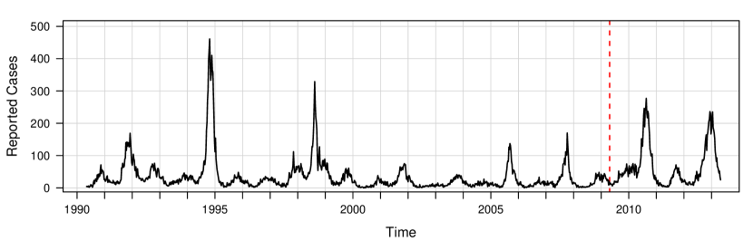
Figure 1: Weekly numbers of reported dengue cases in San Juan, Puerto Rico, 1990–2013. The dashed line marks the boundary between training and test data.

2.2 Viral gastroenteritis incidence in Berlin, Germany

Norovirus and rotavirus are common causes of viral gastroenteritis and can be transmitted from person to person or via contaminated food and items. The average serial interval of norovirus is 3–4 days (Richardson et al., 2001), but the virus may be shed for up to three weeks after symptom resolution (Heymann, 2015). For rotavirus the average serial interval is 5–6 days (Richardson et al., 2001), with infectiousness lasting for up to 12 days (Centers for Disease Control and Prevention, 2015). For rotavirus a vaccine has been available since 2006, while this is not the case for norovirus. In Germany both diseases are notifiable and the Robert Koch Institute makes weekly numbers of reported cases available (https://survstat.rki.de). We consider counts from the twelve districts of Berlin from week 2011-W01 through 2017-W52 (downloaded on 30 Aug 2018). For both diseases we will assess the predictive performance over the weeks 2015-W01 through 2017-W52 (156 weeks) based on at least four years (208 weeks) of training data. Figure 2 shows the observed incidence aggregated to city-wide weekly counts (panels a and b) and the spatial distribution across the twelve districts (panels c and d). For illustration we also show counts from Pankow and Spandau, Berlin’s largest and smallest districts, respectively (panels e–h; see the Supplementary Material for the other districts). Note that parts of the norovirus data have been previously analysed with first-order EE models (Meyer and Held, 2017; Held et al., 2017).

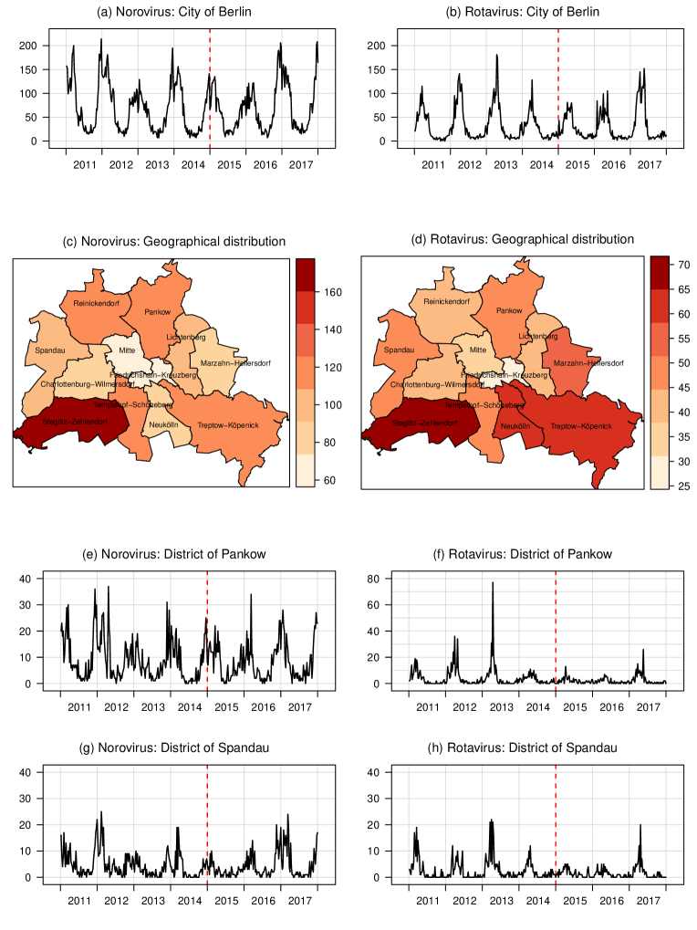
Figure 2: Weekly numbers of reported norovirus (left) and rotavirus (right) cases in Berlin, 2011–2017. Top row: Pooled over the twelve city districts. Second row: Average number of cases per year and 100,000 inhabitants in the twelve districts. Third and fourth row: Districts of Pankow and Spandau. Dotted lines show the beginning of the test period. Plots for the remaining districts can be found in the Supplementary Material.

3 Methodology

3.1 The endemic-epidemic model

We provide a brief overview on the current state of the endemic-epidemic (EE) framework. Given the past, the number of cases $Y_{it}$ in unit $i=1,\dots,m$ and week $t$ is assumed to follow a negative binomial distribution

$$Y_{it}\,|\,\mathbf{Y}_{t-1},\mathbf{Y}_{t-2},\dots \sim\operatorname{NBin}(\lambda_{it},\psi_{i})$$ (1)

with conditional mean $\lambda_{it}$ and overdispersion parameter $\psi_{i}$. The conditional variance is thus $\lambda_{it}+\psi_{i}\lambda_{it}^{2}$ and reduces to $\lambda_{it}$ for $\psi_{i}=0$. A common simplification is to assume one global overdispersion parameter, i.e. $\psi_{i}=\psi$ for $i=1,\dots,m$. Counts from different units $i$ and $j$ at time $t$ are assumed to be conditionally independent given the past.

The conditional mean $\lambda_{it}$ in (1) is further decomposed into

$$\lambda_{it} =\nu_{it}+\phi_{it}\sum_{j=1}^{m}\lfloor w_{ji}\rfloor Y_{j,t-1},$$ (2)

where $\nu_{it}$ is referred to as the endemic component and captures infections not directly linked to observed cases from the previous week. The remaining autoregressive term in (2) is the epidemic component and describes how the incidence in region $i$ is linked to previous cases $Y_{j,t-1}$ in units $j=1,\dots,m$. The parameters $\nu_{it}$ and $\phi_{it}$ are constrained to be non-negative and modelled in a log-linear fashion, for instance with sine-cosine terms to account for seasonality (Held and Paul, 2012). Long-term temporal trends and covariates such as meteorological conditions (Cheng et al., 2016; Bauer and Wakefield, 2018) or vaccination coverage (Herzog et al., 2011) could also be included.

The coupling between units is described by weights $w_{ji}$, which enter in (2) after normalisation: $\lfloor w_{ji}\rfloor=w_{ji}/\sum_{h=1}^{m}w_{jh}$. Unrestricted estimation of all $m^{2}$ weights is usually unstable in practice, so more parsimonious and epidemiologically meaningful parameterizations have been introduced. Specifically, the weights can be based on social contact data for spread across age groups (Meyer and Held, 2017) or on the geographical distance between cases to describe spatio-temporal spread (Meyer and Held, 2014). In the latter case the weights can be specified through a power law

$$w_{ji} =(o_{ji}+1)^{-\rho}$$ (3)

where $o_{ji}$ is the path distance between the regions $j$ and $i$ (with $o_{ii}=0$, $o_{ji}=1$ for direct neighbours $i$ and $j$ and so on) and $\rho$ is a decay parameter to be estimated from the data. The power law formulation is motivated from human movement behaviour (Brockmann et al., 2006) and has been found to be an efficient way of capturing spatial dependence.

3.2 Weighting schemes for past incidence

The EE framework was originally formulated as an observation-driven statistical time series model (Cox, 1981), but a direct derivation from a discrete-time susceptible-infectious-removed (SIR) model has recently been provided by Bauer and Wakefield (2018) and Wakefield et al. (2019). They derive formulation (2) from a competing risks framework where the forces of infection from the infected individuals in units $j=1,\dots,m$ on a susceptible in unit $i$ add up to an overall risk of infection. An important assumption leading to equation (2) is that infectiousness lasts for exactly one time period, and infection at time $t$ is only possible by cases from $t-1$. In other words, the serial interval is fixed to one observation interval. If this assumption is violated, a simple remedy is to aggregate the data to a time scale corresponding to the average serial interval, as done by Herzog et al. (2011) and Wakefield et al. (2019) for measles. This, however, still does not account for the fact that serial intervals are random in reality and vary across infection events. This can be included in the model via an autoregression on several past observations, where the (discretized) distribution of the serial intervals is reflected in the weights assigned to the different lags (Forsberg White and Pagano 2008, Becker 2015, p.156).

Moreover, it has been shown that underreporting can introduce dependencies at higher lags, even if the underlying process is a first-order autoregression (Bracher, 2019). External drivers such as meteorological conditions may have similar effects. This means that even for diseases with typically short serial intervals, including higher-order lags may yield improved predictive performance. At the same time, confounding by such factors implies that there may not always be direct correspondence between the estimated lag weights and the serial interval distribution.

We start by considering univariate EE model with time-constant endemic and epidemic parameters $\nu$ and $\phi$, respectively, which we extend to

$$\lambda_{t}=\nu+\phi\sum_{d=1}^{p}\lfloor u_{d}\rfloor Y_{t-d}.$$ (4)

Here, the weights $\lfloor u_{d}\rfloor=u_{d}/\sum_{g=1}^{p}u_{g}$ are normalized and restricted to be positive. This is in line with the motivation from a discrete-time serial interval distribution (where $\lfloor u_{d}\rfloor$ is the probability for a serial interval of $d$ weeks), but also has technical reasons. The sum-to-one constraint is required for identifiability while positivity of the weights ensures well-definedness of the model (allowing $u_{d}<0$ can result in negative $\lambda_{t}$, in which case the negative binomial distribution is not defined).

Estimating the normalized weights $\lfloor u_{d}\rfloor$ without further parametric assumptions is the most flexible approach, but the large number of additional parameters may lead to numerical instabilities and suboptimal predictive performance. The other extreme is to work with a pre-specified weighting scheme based on epidemiological knowledge. For instance Wang et al. (2011) fix the weights at $u_{1}=5/6,u_{2}=1/6$ in their study on hand, mouth and foot disease, which is considered a plausible description of the infectious period. As a flexible compromise between these two approaches we will moreover consider parametric weighting schemes corresponding to different shapes of the (discrete-time) serial interval distribution (Becker, 2015, p.156). This is combined with data-driven estimation of an underlying scalar parameter.

Specifically, we employ the following three parameterizations, always truncated to lags $d=1,\dots,p$ and depending on an unknown weighting parameter $\kappa$. Shifted Poisson weights correspond to

$$u_{d}=\frac{\kappa^{d-1}}{(d-1)!}\exp(-\kappa),\ \ \kappa>0,$$ (5)

as used by Kucharski et al. (2014) to analyse daily avian influenza data. A linear decay of the weights (subject to a non-negativity constraint),

$$u_{d}=\max(1-\kappa d,0),\ \ 0<\kappa<1,$$ (6)

corresponds to a triangular serial interval distribution. Finally, a geometric weighting scheme

$$u_{d}=(1-\kappa)^{d-1}\kappa,\ \ 0<\kappa<1,$$ (7)

is considered. The latter can also be motivated by the impact underreporting has on the autocorrelation of a first-order autoregressive process (Bracher, 2019). Moreover note that the formulation (4) with geometric weights (7) and $p\rightarrow\infty$ is equivalent to the negative binomial INGARCH(1, 1) model

$$\lambda_{t}=\alpha+\beta Y_{t-1}+\gamma\lambda_{t-1},$$ (8)

where $\alpha=\nu\kappa,\beta=\phi\kappa$ and $\gamma=1-\kappa$ (Fokianos et al., 2009; Zhu, 2011).

Parameterizations (6) and (7) force the weight $u_{1}$ to be the largest and imply a decay in infectiousness. This is reasonable for weekly data and diseases with short serial intervals. The Poisson version (5) can also capture an initial increase in infectiousness and may thus be more appropriate for longer serial intervals or daily data. For comparison we will also consider the current first-order EE formulation where all weight is concentrated on the first lag,

$$u_{1}=1,u_{2}=\ldots=u_{p}=0.$$ (9)

We may also combine the multivariate formulation (2) with the suggested weighting schemes,

$$\lambda_{it} =\nu_{it}+\phi_{it}\sum_{d=1}^{p}\sum_{j=1}^{m}\lfloor u_{d}\rfloor\lfloor w_{ji}\rfloor Y_{j,t-d},$$ (10)

where $\nu_{it}$ and $\phi_{it}$ now depend on unit $i$ and time $t$. The weights $\lfloor u_{d}\rfloor$, however, are assumed to be constant across units and time.

3.3 Inference

We have extended the likelihood-based inference procedure from the R package surveillance (Meyer et al., 2017) to fit higher-order lag models (5)–(7) in the package hhh4addon (see A). To optimize the likelihood given the weights $\lfloor u_{d}\rfloor$, the efficient and robust routine provided in surveillance for first-order models (Paul et al., 2008; Paul and Held, 2011; Meyer and Held, 2014) has been adapted. To facilitate integration with the existing implementation, the weighting parameter $\kappa$ (suitably transformed to the real line) or the unrestricted weights $\lfloor u_{d}\rfloor$ (on a multinomial logit scale) are estimated via a profile likelihood approach (Held and Sabanés Bové, 2014). This way, there is no need to implement cumbersome derivatives of the log likelihood function with respect to the additional parameters. Note that a similar approach has previously been applied to fit EE models with an additional age stratification (Meyer et al., 2017).

The maximum of the profile likelihood function can be found using standard numerical optimization. If the weights are estimated in an unrestricted nonparametric manner it may be necessary to try several starting values to ensure convergence. This is also the case for the triangular parameterization (6), which sometimes leads to several local optima (see remarks in Section 4.2.1).

Under the parametric formulations (5)–(7), the weights $\lfloor u_{d}\rfloor$ usually become negligible after a certain order. To find a sufficiently large $p$ we suggest to inspect the weights visually and to plot the order $p$ against the AIC (or log-likelihood, as the complexity of the model does not depend on $p$) to check when changes become negligible. For the unrestricted estimation of the weights $\lfloor u_{1}\rfloor,\dots,\lfloor u_{p}\rfloor$, where the number of model parameters depends on $p$, we choose the order based on the AIC, as is common for prediction purposes.

3.4 Prediction and predictive model assessment

In order to take into account the uncertainty surrounding epidemiological forecasts, these should take the form of predictive distributions rather than deterministic point forecasts (Held et al., 2017). We consider weekly updated forecasts for different horizons $h=1,\dots,H$, as in the recent CDC FluSight challenge (McGowan et al., 2019). This means that for each week $t$, the model is re-fitted using all data already available in order to predict the incidence in weeks $t+1,\dots,t+H$. As in previous work (Held and Meyer, 2019) we use plug-in forecasts, i.e. forecast from the fitted model without carrying forward the uncertainty in the parameter estimates. Taking this into account would require fitting EE models using MCMC methods in a Bayesian framework (Bauer and Wakefield, 2018; Wakefield et al., 2019) with carefully chosen prior distributions.

Plug-in one-week-ahead forecast distributions from EE models are given by independent negative binomial distributions for the $m$ units, so the predictive densities can be evaluated analytically. For forecast horizons of two or more weeks ahead, predictive means, variances and autocovariances can be still obtained analytically in the EE class, see the Supplementary Material for details. The full predictive distributions, however, are no longer given by any standard distribution and are dependent across different units, as they reflect e.g. spatio-temporal dependencies arising over a longer forecast horizon. To evaluate the predictive probability masses $f(\mathbf{Y}_{t+h}\,|\,M)$ we apply the following procedure, which uses Rao-Blackwellization (Gelfand and Smith, 1990; Ray et al., 2017) for improved numerical stability:

1. Generate $k=1,\ldots,K$ samples from the predictive distribution of
   $(\mathbf{Y}_{t+1},\dots,\mathbf{Y}_{t+h-1}\,|\,M)$.

2. For each sample $(\mathbf{y}_{t+1}^{(k)},\dots\mathbf{y}_{t+h-1}^{(k)})$ and each unit $i=1,\dots,m$ evaluate

   $$f(Y_{i,t+h}\,|\,M,\mathbf{y}_{t+1}^{(k)},\dots,\mathbf{y}_{t+h-1}^{(k)})$$

   on a suitably chosen support $y_{i,t+h}\in\{0,\dots,Y_{i,t+h}^{(\text{max})}\}$. These one-week-ahead distributions are conditionally independent negative binomial distributions. The joint probability mass function $f(\mathbf{Y}_{t+h}\,|\,M,\mathbf{y}_{t+1}^{(k)},\dots,\mathbf{y}_{t+h-1}^{(k)})$ is thus given by the product of the unit-wise probability mass functions.

3. Compute $f(\mathbf{Y}_{t+h}\,|\,M)=1/K\cdot\sum_{k=1}^{K}f(\mathbf{Y}_{t+h}\,|\,M,\mathbf{y}_{t+1}^{(k)},\dots,\mathbf{y}_{t+h-1}^{(k)})$.

As the relevant support of $\mathbf{Y}_{t+h}$ obviously gets very large even for moderate $m$, we usually only store the unit-wise marginal predictive densities or summaries thereof (central 50% and 95% predictive intervals), supplemented with analytically obtained covariances. In all applications we set $K=1000$, which led to very stable results.

To assess the performance of probabilistic forecasts, proper scoring rules (Gneiting and Raftery, 2007) have become the standard in infectious disease epidemiology (Held et al., 2017). A score is called proper if there is no incentive for a forecaster to digress from her true belief, and strictly proper if any such digress leads to a penalty. A commonly used strictly proper score is the logarithmic score

$$\text{logS}(y_{\text{obs}}\,|\,M)=-\log[f(y_{\text{obs}}\,|\,M)],$$

i.e. the negative log predictive probability mass the model $M$ assigned to the observed value $y_{\text{obs}}$. The score is negatively oriented, i.e. lower values are better. To aggregate over several forecasts one can use average log scores, which are still strictly proper. For multivariate $h$-week ahead forecasts of $\mathbf{Y}_{t+h}$ we apply the multivariate logarithmic score (Gneiting et al., 2008)

$$\text{logS}(\mathbf{y}_{t+h}\,|\,M)=-\log[f(\mathbf{y}_{t+h}\,|\,M)]$$ (11)

where $M$ is now a model fitted based on the information available at time $t$. In practice the score (11) is often standardized and divided by $m=\text{dim}(\mathbf{y}_{t})$. For one-week-ahead predictions from EE models, the standardized multivariate log score can be evaluated analytically as it is just the average of $m$ negative binomial log-densities. For $h\geq 2$ we apply the simulation-based approach described above.

3.5 Reference forecasts

Throughout this manuscript we will compare our methods to two other forecasting approaches. The first is a naïve seasonal model which does not take into account any serial dependence. It is given by a negative binomial generalized linear model (GLM) including the calendar week and, in the multivariate case, district as categorical covariates (fitting separate models per district was not possible as the frequent zero counts in our data led to degenerate forecast distributions). The second reference model is the negative binomial GLARMA (generalized linear autoregressive moving average) model implemented in the R package glarma (Dunsmuir and Scott, 2015). In contrast to the EE model, the GLARMA model also allows for negative dependencies between observations. As in Held and Meyer (2019) we fitted this model with the same sine-cosine terms for seasonality as the respective EE models. Details on the GLARMA model are provided in the Supplementary Material.

4 Applications

4.1 Incidence of dengue fever in San Juan, Puerto Rico

Ray et al. (2017) compare the predictive performance of the EE model framework with their kernel conditional density estimation (KCDE) method. They apply the following first-order EE model to the weekly dengue counts described in Section 2.1:

$$\lambda_{t} =\nu_{t}+\phi_{t}Y_{t-1}$$ (12)

$$\log(\nu_{t}) =\alpha^{(\nu)}+\gamma^{(\nu)}\sin(2\pi t/\omega)+\delta^{(\nu)}\cos(2\pi t/\omega)$$ (13)

$$\log(\phi_{t}) =\alpha^{(\phi)}+\sum_{k=1}^{2}\gamma_{k}^{(\phi)}\sin(2\pi kt/\omega)+\delta_{k}^{(\phi)}\cos(2\pi kt/\omega),$$ (14)

where $\omega=52$ to model yearly seasonality in weekly data. This formulation has been chosen by Ray et al. (2017) from a number of candidate models based on the AIC on the training data (1990-W18 through 2009-W17, see Figure 1). Note that unlike in other works on dengue (Cheng et al., 2016; Chen et al., 2019), Ray et al. (2017) do not incorporate meteorological data. To ensure comparability with Ray et al. (2017) we only replace (12) with (4) but stick to the decomposition of $\log(\nu_{t})$ and $\log(\phi_{t})$ as in (13) and (14). For the weights $\lfloor u_{d}\rfloor$ we apply unrestricted nonparametric estimation and the parametric formulations (5)–(7). In addition, we use a weighting scheme based on an estimate of the serial interval distribution from Siraj et al. (2017, Fig. 1). Discretized to a weekly scale, it is given by $u_{1}=0,u_{2}=0.2,u_{3}=0.425,u_{4}=0.25,u_{5}=0.125$. On a standard laptop the model fitting takes around one second per model for the parametric versions and four seconds for the unrestricted one. We did not re-run the KCDE forecasts from Ray et al. (2017), since their extensive Supplementary Material (https://github.com/reichlab/article-disease-pred-with-kcde) allowed us to compute all quantities required in our comparison. However, previous studies (Held and Meyer, 2019) indicate that KCDE requires at least an order of magnitude more computation time than the EE approach.

4.1.1 Model fit and residual correlation

Figure 3, left panel, shows the AIC values achieved for the training data under the different parameterizations of the lag weights and orders $p$ relative to the first-order EE model (AIC = 6671.1) used in Ray et al. (2017; we omit comparison to the KCDE method here as no AIC values are available). The largest improvement ($\Delta\mbox{AIC}=-117.1$) is achieved by a model with $p=4$ and unrestricted weights $\lfloor u_{d}\rfloor$. For all parametric versions (5)–(7) the AIC stays practically constant from $p=5$ on, with the geometric version performing better ($\Delta\mbox{AIC}=-112.2$) than the Poisson and triangular versions ($\Delta\mbox{AIC}=-97.5$ and $-96.3$, respectively). The model using the serial interval distribution from Siraj et al. (2017, referred to as literature in the legend) is omitted here as it has a considerably higher AIC ($\Delta\text{AIC}=186$ relative to the first-order model).

The weights $\lfloor u_{d}\rfloor$ resulting from the different parameterizations are shown in the middle panel of Figure 3 (with $p=4$ for the nonparametric version and $p=5$ otherwise). The unrestricted weights show a non-monotonic pattern where the third lag is more important than the second. The parametric weights all imply decaying weights, with the geometric version assigning more weight to lags 4 and 5 than two than the Poisson and triangular ones. These results are in contrast to the weights based on the serial interval distribution from Siraj et al. (2017), indicating that other factors like meteorological conditions also impact the autocorrelation structure and thus the estimated lag weights. Plots of the profile likelihood for each parameterization can be found in the Supplementary Material.

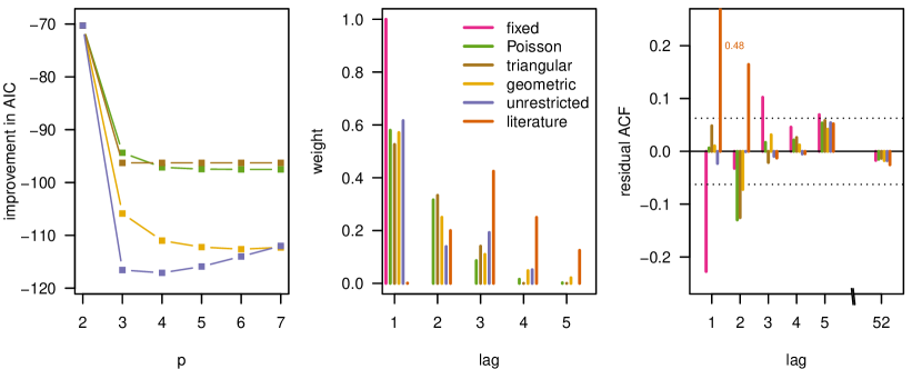
Figure 3: Left: Improvement in AIC (relative to the first-order EE model) for the different lag weight parameterizations and values of $p$, applied to dengue counts 1990–2009. Middle: Weights $\lfloor u_{d}\rfloor$ (with $p=4$ in the unrestricted case, $p=5$ otherwise). Right: Autocorrelations of Pearson residuals. The model denoted by literature is based on the serial interval distribution from Siraj et al. (2017).

The autocorrelation functions of the Pearson residuals $(y_{t}-\lambda_{t})/\sqrt{\lambda_{t}+\psi\lambda_{t}^{2}}$ shown in the right panel of Figure 3 look unsuspicious for the nonparametric and the geometric versions. The simpler first-order model suffers from strong negative autocorrelation at lag 1, while for the Poisson and triangular serial interval distributions these occur at lag 2. These patterns are in line with the fact that relative to the nonparametric version these parameterizations assign too much weight to lags one and two, respectively. The model with pre-specified weights based on the serial interval shows excessive residual autocorrelations at lag one, likely because it does not use the first lag and fails to capture short-time dependencies induced by external factors.

4.1.2 Predictive assessment

We now assess the predictive performance of the different EE models and compare them to the KCDE approach (Ray et al., 2017) and the reference models over the course of the seasons 2009/10 through 2012/13. Unlike Ray et al. (2017), who averaged scores over prediction horizons $1,\dots,52$, we focus on short-term forecasts and assess performance separately for the horizons $h=1,\dots,8$ weeks. For the KCDE method the respective average scores (over the 208 weeks of test data) could be computed from material provided in the Supplement of Ray et al. (2017).

The left panel of Figure 4 shows the average scores obtained by the periodic, full bandwidth KCDE method, the six variants of the EE model, and the two reference models from Section 3.5. The weighting based on the serial interval distribution from Siraj et al. (2017) leads to slight improvements relative to the first-order model for horizons 2 through 6, but considerably worse performance of one-week-ahead forecasts. The EE models with data-driven weighting schemes yield better performance than the first-order version at all horizons, while differences between the four parameterizations are minor. Notably, the unrestricted nonparametric approach does not lead to a performance gain compared to the parametric versions. For one- and two-week ahead predictions the extended EE models also outperform the KCDE method. The differences, shown in detail in the right panel of Figure 4, may be spurious, however. Permutation tests (Paul and Held, 2011) indicate only weak evidence that the forecasts from the extended EE models actually perform better (two-sided $p$-values between 0.05 and 0.18 for $h=1$ and 0.06 and 0.13 for $h=2$). While for $h=3$ performance is almost identical, from $h=4$ onwards there is moderate to strong evidence that KCDE performs better ($p$-values of 0.04 and smaller; see Supplementary Material). A possible reason is that KCDE uses separate models optimized for prediction at different horizons, while the EE method generates all forecasts iteratively from the same model. Concerning the reference models, the naïve seasonal model is clearly outperformed by all other approaches. The GLARMA model performs very similarly to the higher-order EE models for one-week-ahead forecasts, somewhat worse for horizons 2 through 4 and somewhat better for horizons 6 through 8 (but worse than KCDE).

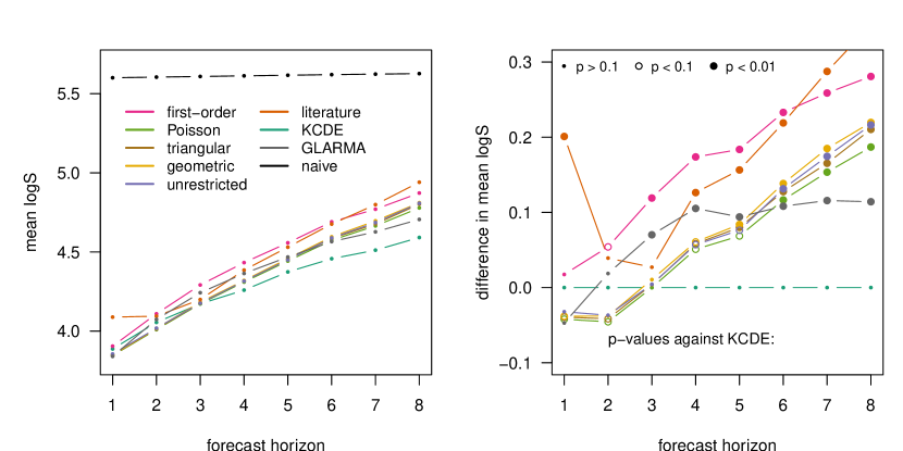
Figure 4: Left: average log scores of dengue forecasts at horizons $h=1,\dots,8$. Right: differences in average log scores compared to KCDE (negative values indicate better performance of EE methods). The point shape in the right plot indicates whether there is evidence for different forecasting performance of KCDE and the respective EE method (based on two-sided $p$-values from permutation tests; Paul and Held 2011). All numbers underlying this figure can be found in the Supplementary Material.

Visualizations of forecasts from different models and at different horizons can be found in the Supplementary Material. We here restrict ourselves to a comparison of the central 50% and 95% prediction intervals from the first-order and geometric lag EE models, shown in the left panel of Figure 5. As they are based on an average of past values rather than just the last, the predictions from the model with geometric weights form a smoother curve. The right panel of the figure moreover shows probability integral transform (PIT) histograms of one-week-ahead and four-week ahead forecasts from the model with geometric weights, i.e. the distribution of $\text{PIT}_{t+h}=\text{Pr}(Y_{t+h}\leq y_{t+h}\,|\,M)$ (with a correction for the discreteness of the data, Czado et al. 2009). If forecasts are well calibrated, the PIT histogram should be approximately uniform, as is the case for a forecast horizon of one week. At a horizon of four weeks, there are too many large PIT values, i.e. observations towards the upper tail of the respective predictive distribution. Note, however, that strictly speaking PIT histograms should be applied to a set of mutually independent forecasts, which is not the case for horizons $h>1$.

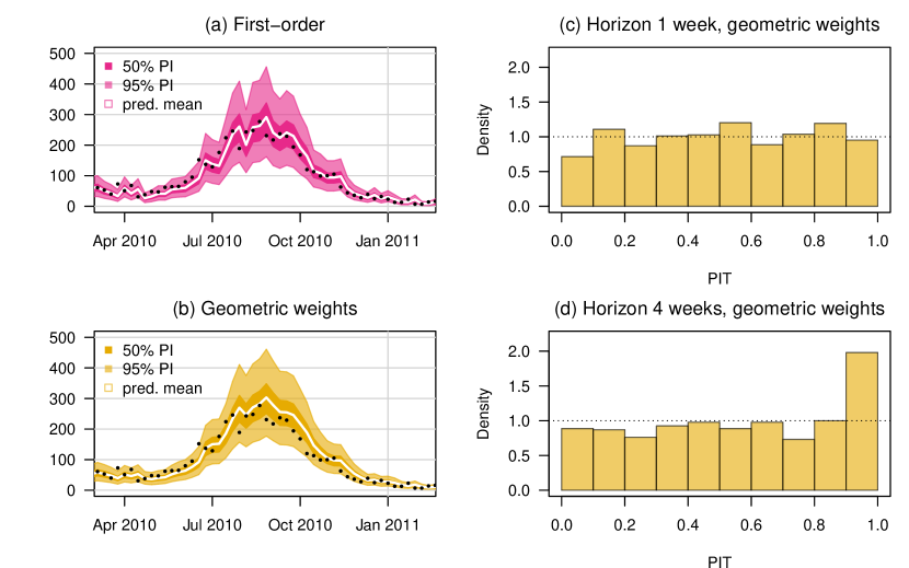
Figure 5: Left: One-week ahead 50% and 95% prediction intervals for dengue, season 2010/2011, obtained from EE models with (a) only first lag and (b) geometric weights. Right: PIT histograms of (c) one-week-ahead and (d) four-week-ahead forecasts from the model with geometric weights.

4.2 Viral gastroenteritis incidence in Berlin, Germany

We now apply multivariate EE models to the data on norovirus and rotavirus in Berlin, weeks 2011–W06 to 2017–W52. We revisit and extend two model variants specified in Held et al. (2017) for district-level norovirus data (there referred to as Models 7 and 8, Section 3.3). To model incidence in the twelve districts, both original models combine the formulation (2) and power law weights (3) to describe spatial spread. The overdispersion parameter $\psi$ is shared across districts. The first model, which we refer to as the full model, is defined as

$$\log(\nu_{it}) =\alpha^{(\nu)}_{i}+\beta^{(\nu)}x_{t}+\gamma^{(\nu)}\sin(2\pi t/\omega)+\delta^{(\nu)}\cos(2\pi t/\omega)$$ (15)

$$\log(\phi_{it}) =\alpha^{(\phi)}_{i}+\gamma^{(\phi)}\sin(2\pi t/\omega)+\delta^{(\phi)}\cos(2\pi t/\omega),$$ (16)

where again $\omega=52$. It features shared terms $\beta^{(\nu)},\gamma^{(\cdot)}$ and $\delta^{(\cdot)}$ for seasonality, but district-specific intercepts $\alpha^{(\cdot)}_{i}$ in both the endemic and the epidemic parameters. As in Held et al. (2017), the indicator $x_{t}$ for calendar weeks 52 and 1 aims to capture changes in reporting behaviour or social contact patterns during the Christmas break, as quantified by the coefficients $\beta^{(\nu)}$. Note that the same indicator has also been included into the GLARMA reference model.

The second model is more parsimonious and features a gravity model component (Xia et al., 2004) instead of district-specific intercepts in the epidemic component. Equation (16) is thus replaced by

$$\log(\phi_{it}) =\alpha^{(\phi)}+\tau^{(\phi)}\log(e_{i})+\gamma^{(\phi)}\sin(2\pi t/\omega)+\delta^{(\phi)}\cos(2\pi t/\omega),$$ (17)

where $e_{i}$ is the fraction of the total population living in district $i$. The amount of disease transmission thus scales with the population size of the ‘importing’ district (Meyer et al., 2017).

As mentioned in Section 2.2, epidemiological knowledge on both diseases suggests that serial intervals may exceed one week. Also, it is known that gastrointestinal diseases are subject to considerable underreporting (Tam et al., 2012) as well as meteorological influences (Patel et al., 2013). Consequently, we expect dependencies at higher lags and replace formulation (2) by the more flexible (10). Again, we apply nonparametric estimation of the lag weights and the three parametric versions (5)–(7). For comparison we apply the first-order formulation (9) as well as the reference models from Section 3.5.

4.2.1 Model fit and residual correlation

We start by contrasting some features of the model fits with and without weighting of past incidence. As the available time series are shorter here we use the full data set to obtain more reliable estimates. For the parametric serial weights the fitting took around four seconds per model on a standard laptop, while the unrestricted nonparametric versions took one minute. We chose $p=5$ as for both diseases and model versions (full and gravity) the AIC values for $p>5$ stayed constant for all parametric versions and increased for the nonparametric one, see Figures in the Supplementary Material. We also show plots of the profile likelihoods for the three parametric weighting schemes. The triangular version shows several local maxima for rotavirus, indicating that optimization has to be done with care under this parameterization (we adopt a grid-based optimization in the following to avoid getting stuck in local optima).

Table 1 indicates that for both norovirus and rotavirus the model performance improves when weights for past incidence are included, with the geometric version performing best. For both diseases, this extension leads to a stronger improvement than modelling cross-district dependencies more flexibly (when moving from the gravity to the full model). This emphasizes the importance of including the information contained in observations from two or more weeks back in time.

Table 1: Differences in AIC relative to the first-order version of the gravity model (negative values indicate improvement).

	Norovirus		Rotavirus
Weighting	gravity	full	gravity	full
scheme	model	model	model	model
first-order	0.0	-63.5	0.0	-35.9
Poisson	-120.7	-171.3	-78.7	-106.9
triangular	-118.0	-168.1	-74.8	-102.5
geometric	-125.9	-174.2	-93.3	-118.2
unrestricted	-123.0	-169.6	-92.9	-117.3

Figure 6: Estimated weights $\lfloor u_{d}\rfloor$, total endemic component $\sum_{i=1}^{12}\nu_{it}$, decay parameter $\rho$ of the spatial power law and overdispersion parameter $\psi$ for the full model with different lag weighting schemes.

In the remainder of this subsection we focus on the full model which showed better in-sample performance than the gravity model. Figure 6 shows selected features of models with different weight parameterizations. The weights $\lfloor u_{d}\rfloor$, shown in the first column, are similar for the two diseases, despite the differences in average serial intervals mentioned in Section 2.2. Under all four parameterizations, the first lag receives a weight slightly below 0.6. For both diseases the geometric weights mimic best the relatively slow decay in the unrestricted weights, explaining its good AIC values. As shown in the second column of Figure 6, including the weighting schemes reduces the total endemic component $\sum_{i=1}^{12}\nu_{it}$ considerably. A larger part of the incidence is thus explained by previous dynamics, which is a sign of improved model fit. Note that the lower values in calendar weeks $1$ and $52$ are due to the Christmas break. The power law decay parameters $\rho$ increase when lag weights are included (third column of Figure 6), meaning that the model borrows slightly less information across regions. Finally, the overdispersion parameters $\psi$ are lower for the extended models, indicating less unexplained variability (fourth column).

The first-order models lead to some significant residual autocorrelations at lags two and three (plots shown in the Supplementary Material). These largely disappear in the extended models.

4.2.2 Predictive model assessment

We assess the predictive performance of the different model variants for the period 2015-W01–2017-W52. Again, we re-fitted models each week including the most recent data. However, we chose the order $p$ only once based on the training data (2011-2014, 208 weeks). As for the models fitted to the full seven years of data in Section 4.2.1 this led to $p=5$ for all parametric versions and the nonparametric version for rotavirus. For the norovirus model with nonparametric lag weights, however, $p=3$ resulted in the best AIC on the training data, so that we used this value.

Table 2 shows the average standardized multivariate log scores of one-week ahead forecasts for the norovirus and rotavirus time series (over the 156 weeks of test data). For norovirus, the additional flexibility of the full model seems to lead to somewhat improved predictive performance, but permutation tests indicate only weak evidence for an actual difference ($p$-values between 0.097 and 0.19 for the different parameterizations). For rotavirus both model variants perform very similarly ($p$-values $\geq$ 0.57).

Table 2: Differences in mean standardized log scores of one-week-ahead forecasts over years 2015–2017, relative to the first-order gravity model (negative values indicate improvement). The two last rows provide results for the reference models.

	Norovirus		Rotavirus
Weighting	gravity	full	gravity	full
scheme	model	model	model	model
first-order	0.000	-0.006	0.000	0.003
Poisson	-0.015	-0.021	-0.017	-0.015
triangular	-0.014	-0.020	-0.012	-0.014
geometric	-0.017	-0.022	-0.019	-0.018
unrestricted	-0.015	-0.020	-0.016	-0.014
GLARMA		0.000		0.011
naive		0.091		0.090

The inclusion of the lag weighting schemes, on the other hand, very consistently improves the predictive performance, with the geometric version yielding the best results. There is strong evidence that the latter predicts better than the respective first-order version for both model variants and diseases ($p$-values of around 0.001). However, there is only weak evidence for a performance difference between the geometric and the other other weighting schemes ($p$-values between 0.07 and 0.09 and between 0.07 and 0.11 for the full norovirus and rotavirus models, respectively).

All EE models clearly outperform the naïve seasonal models. The performance of the GLARMA model is similar to that of the first-order gravity model for norovirus and somewhat worse for rotavirus. Permutation tests indicate that the GLARMA approach is outperformed by the higher-order EE models ($p$-values of 0.002 or below when compared to the respective full geometric weight model).

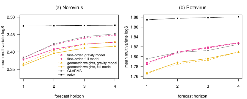
Figure 7: Average standardized multivariate log scores for norovirus and rotavirus forecasts at horizons $h=1,2,3,4$ weeks. Results are shown for first-order models and models with geometric weights. The naïve seasonal and the GLARMA model are shown for comparison.

Finally we compare the forecast performance of first-order EE models and models with geometric lag weights for horizons up to four weeks. Average standardized multivariate log scores over the test period are shown in Figure 7. For norovirus, the full model performs better than the gravity model also for horizons $h\geq 2$ ($p$-values of 0.062 and below), while for rotavirus the differences are again negligible. For both diseases and model versions, permutation tests indicate strong evidence that the geometric parameterization improves prediction at horizons $h=2,3,4$ ($p$-values ranging from $<0.0001$ to 0.007 for the two diseases and model versions). For norovirus the improvement corresponds roughly to the difference between two- and three-week-ahead forecasts. For rotavirus, it is even more pronounced as it corresponds to the difference between one- and three-week-ahead forecasts. Also at higher horizons, the GLARMA model yields similar performance as the first-order gravity model, while the naïve model performs considerably worse than all other approaches.

5 Discussion

In this article we have extended the endemic-epidemic framework to include weighting schemes for past incidence which are inspired by discrete-time serial interval distributions. In both case studies the proposed parameterizations led to considerably improved model fits, with the geometric scheme performing best. These improvements also translated to improved predictive performance at various forecasting horizons. There was no additional benefit in estimating the lag weights in an unrestricted nonparametric manner. The parametric formulations are therefore an attractive option for practical analyses and forecasts. As optimization of the log-likelihood function turned out to be more difficult for the triangular weights and performance tended to be slightly weaker, we consider the geometric and shifted Poisson versions preferable.

Our model extension is motivated from serial interval distributions, but some remarks are warranted. Firstly, as mentioned before, the weights $u_{d}$ are not only shaped by the serial interval distribution, but also other factors. These have to be taken into account if the purpose of an analysis is estimation of serial intervals rather than prediction. Moreover, to obtain valid estimates of transmission parameters, the observation interval needs to be chosen in a suitable way (Nishiura et al., 2010; Reich et al., 2016), ideally similar or shorter than the serial interval. For prediction purposes, however, this is not crucial, as the EE model can adapt to the increased dispersion resulting from within-week dynamics via its overdispersion parameter. We therefore think that our model extension is applicable to short-term forecasting of a wide range of diseases with short to medium-length serial intervals.

A property of the proposed formulation is that the weighting parameter $\kappa$ is assumed to be time-constant and identical across units, which is motivated from the assumption of time-invariant serial interval distributions. This may be restrictive in some applications, for instance due to time-varying social contact patterns, meteorological conditions and dominant strains. However, while in principle it would be possible to allow for a time-varying $\kappa_{t}$, we expect identifiability to be poor. Sometimes the EE framework is also applied to analyse two diseases jointly (Paul et al., 2008; Chiavenna et al., 2019), in which case using separate parameters $\kappa_{i}$ could be of interest. In spatio-temporal settings as in our work, however, we prefer to use one shared parameter $\kappa$.

In the present article we only assessed the forecasting performance for $h$-week ahead forecasts. Other potential forecast targets include the entire incidence curve over a season (Held et al., 2017) or more specific features like the onset timing, peak timing and peak incidence (Ray et al., 2017; McGowan et al., 2019). These, too, are expected to be dependent across geographical sub-units. It would therefore be of interest to generate and evaluate forecasts in a multivariate fashion as illustrated for $h$-week ahead forecasts in the present article. But even if forecasts are only evaluated at a univariate aggregate level, initial modelling at a finer resolution is a promising strategy which can improve forecasts (Held et al., 2017).

Appendix A Software and reproducibility

Software for model fitting and forecasting is provided in the R package hhh4addon which extends the functionality of the surveillance package (Meyer et al., 2017). It is available at https://github.com/jbracher/hhh4addon. The package also contains the data presented in Section 2, which were obtained from the web platform of the Robert Koch Institute (https://survstat.rki.de) and the Supplementary Material of Ray et al. (2017). Codes to reproduce the presented analyses are available at https://github.com/jbracher/dengue_noro_rota.

References

- Adegboye et al. (2017) Adegboye, O., M. Al-Saghir, and D. Leung (2017). Joint spatial time-series epidemiological analysis of malaria and cutaneous leishmaniasis infection. Epidemiology and Infection 145(4), 685–700.
- Aldstadt et al. (2012) Aldstadt, J., I. Yoon, D. Tannitisupawong, R. Jarman, S. Thomas, R. Gibbons, A. Uppapong, S. Iamsirithaworn, A. Rothman, T. Scott, and T. Endy (2012). Space-time analysis of hospitalised dengue patients in rural Thailand reveals important temporal intervals in the pattern of dengue virus transmission. Tropical Medicine & International Health 17(9), 1076–1085.
- Bauer and Wakefield (2018) Bauer, C. and J. Wakefield (2018). Stratified space-time infectious disease modelling, with an application to hand, foot and mouth disease in China. Journal of the Royal Statistical Society, Series C, Applied Statistics 67(5), 1379–1398.
- Bauer et al. (2016) Bauer, C., J. Wakefield, H. Rue, S. Self, Z. Feng, and Y. Wang (2016). Bayesian penalized spline models for the analysis of spatio-temporal count data. Statistics in Medicine 35(11), 1848–1865.
- Becker (2015) Becker, N. (2015). Modeling to Inform Infectious Disease Control. Boca Raton, FL: CRC Press.
- Bracher (2019) Bracher, J. (2019). Comment on “Under-reported data analysis with INAR-hidden Markov chains”. Statistics in Medicine 38(5), 893–898.
- Brockmann et al. (2006) Brockmann, D., L. Hufnagel, and T. Geisel (2006). The scaling laws of human travel. Nature 439(7075), 462–465.
- Centers for Disease Control and Prevention (2015) Centers for Disease Control and Prevention (2015). Epidemiology and Prevention of Vaccine-Preventable Diseases. Washington, D.C.: Public Health Foundation.
- Chen et al. (2019) Chen, C. W. S., K. Khamthong, and S. Lee (2019). Markov switching integer-valued generalized auto-regressive conditional heteroscedastic models for dengue counts. Journal of the Royal Statistical Society: Series C (Applied Statistics) 68(4), 963–983.
- Cheng et al. (2016) Cheng, Q., X. Lu, J. Wu, Z. Liu, and J. Huang (2016). Analysis of heterogeneous dengue transmission in Guangdong in 2014 with multivariate time series model. Scientific Reports 6, Article No. 33755.
- Chiavenna et al. (2019) Chiavenna, C., A. M. Presanis, A. Charlett, S. de Lusignan, S. Ladhani, R. G. Pebody, and D. De Angelis (2019). Estimating age-stratified influenza-associated invasive pneumococcal disease in England: A time-series model based on population surveillance data. PLOS Medicine 16(6), 1–21.
- Cox (1981) Cox, D. (1981). Statistical analysis of time series. Some recent developments. Scandinavian Journal of Statistics 8, 93–115.
- Cui and Zhu (2018) Cui, Y. and F. Zhu (2018). A new bivariate integer-valued GARCH model allowing for negative cross-correlation. TEST 27(2), 428–452.
- Czado et al. (2009) Czado, C., T. Gneiting, and L. Held (2009). Predictive model assessment for count data. Biometrics 65(4), 1254–1261.
- Del Valle et al. (2018) Del Valle, S. Y., B. H. McMahon, J. Asher, R. Hatchett, J. C. Lega, H. E. Brown, M. E. Leany, Y. Pantazis, D. J. Roberts, S. Moore, A. T. Peterson, L. E. Escobar, H. Qiao, N. W. Hengartner, and H. Mukundan (2018). Summary results of the 2014-2015 DARPA Chikungunya Challenge. BMC Infectious Diseases 18(1), 245.
- Dunsmuir and Scott (2015) Dunsmuir, W. and D. Scott (2015). The glarma package for observation-driven time series regression of counts. Journal of Statistical Software, Articles 67(7), 1–36.
- Fokianos et al. (2009) Fokianos, K., A. Rahbek, and D. Tjøstheim (2009). Poisson autoregression. Journal of the American Statistical Association 104(488), 1430–1439.
- Fokianos et al. (2020) Fokianos, K., B. Støve, D. Tjøstheim, and P. Doukhan (2020, 02). Multivariate count autoregression. Bernoulli 26(1), 471–499.
- Forsberg White and Pagano (2008) Forsberg White, L. and M. Pagano (2008). A likelihood-based method for real-time estimation of the serial interval and reproductive number of an epidemic. Statistics in Medicine 27(16), 2999–3016.
- Gelfand and Smith (1990) Gelfand, A. E. and A. F. M. Smith (1990). Sampling-based approaches to calculating marginal densities. Journal of the American Statistical Association 85(410), 398–409.
- Gneiting and Raftery (2007) Gneiting, T. and A. E. Raftery (2007). Strictly proper scoring rules, prediction, and estimation. Journal of the American Statistical Association 102(477), 359–378.
- Gneiting et al. (2008) Gneiting, T., L. I. Stanberry, E. P. Grimit, L. Held, and N. A. Johnson (2008). Assessing probabilistic forecasts of multivariate quantities, with an application to ensemble predictions of surface winds. TEST 17(2), 211–235.
- Heinen and Rengifo (2007) Heinen, A. and E. Rengifo (2007). Multivariate autoregressive modeling of time series count data using copulas. Journal of Empirical Finance 14(4), 564 – 583.
- Held et al. (2005) Held, L., M. Höhle, and M. Hofmann (2005). A statistical framework for the analysis of multivariate infectious disease surveillance counts. Statistical Modelling 5(3), 187–199.
- Held and Meyer (2019) Held, L. and S. Meyer (2019). Forecasting based on surveillance data. In: Held, L, Hens, N, O’Neill, P and Wallinga, J, ed. Handbook of Infectious Disease Data Analysis. London, UK: Chapman & Hall. 2019.
- Held et al. (2017) Held, L., S. Meyer, and J. Bracher (2017). Probabilistic forecasting in infectious disease epidemiology: the 13th Armitage lecture. Statistics in Medicine 36(22), 3443–3460.
- Held and Paul (2012) Held, L. and M. Paul (2012). Modeling seasonality in space-time infectious disease surveillance data. Biometrical Journal 54(6), 824–843.
- Held and Sabanés Bové (2014) Held, L. and D. Sabanés Bové (2014). Applied Statistical Inference: Likelihood and Bayes. Springer, Berlin.
- Herzog et al. (2011) Herzog, S., M. Paul, and L. Held (2011). Heterogeneity in vaccination coverage explains the size and occurrence of measles epidemics in German surveillance data. Epidemiology and Infection 139(4), 505–515.
- Heymann (2015) Heymann, D. (Ed.) (2015). Control of Communicable Diseases Manual (20th ed.). Washington, DC: APHA Press.
- Keeling and Rohani (2008) Keeling, M. and P. Rohani (2008). Modeling Infectious Diseases in Humans and Animals. Princeton, NJ: Princeton University Press.
- Kucharski et al. (2014) Kucharski, A., H. Mills, A. Pinsent, C. Fraser, M. Van Kerkhove, C. Donnelly, and R. S (2014). Distinguishing between reservoir exposure and human-to-human transmission for emerging pathogens using case onset data. PLOS Current Outbreaks.
- Ma et al. (2018) Ma, Y., C. R. Horsburgh, L. F. White, and H. E. Jenkins (2018). Quantifying TB transmission: a systematic review of reproduction number and serial interval estimates for tuberculosis. Epidemiology and Infection 146(12), 1478–1494.
- McGowan et al. (2019) McGowan, C. J., M. Biggerstaff, M. Johansson, K. M. Apfeldorf, M. Ben-Nun, L. Brooks, M. Convertino, M. Erraguntla, D. C. Farrow, J. Freeze, S. Ghosh, S. Hyun, S. Kandula, J. Lega, Y. Liu, N. Michaud, H. Morita, J. Niemi, N. Ramakrishnan, E. L. Ray, N. G. Reich, P. Riley, J. Shaman, R. Tibshirani, A. Vespignani, Q. Zhang, C. Reed, R. Rosenfeld, N. Ulloa, K. Will, J. Turtle, D. Bacon, S. Riley, W. Yang, and T. I. F. W. Group (2019). Collaborative efforts to forecast seasonal influenza in the United States, 2015–2016. Scientific Reports, 683.
- Meyer and Held (2014) Meyer, S. and L. Held (2014). Power-law models for infectious disease spread. Annals of Applied Statistics 8(3), 1612–1639.
- Meyer and Held (2017) Meyer, S. and L. Held (2017). Incorporating social contact data in spatio-temporal models for infectious disease spread. Biostatistics 18(2), 338–351.
- Meyer et al. (2017) Meyer, S., L. Held, and M. Höhle (2017). Spatio-temporal analysis of epidemic phenomena using the R package surveillance. Journal of Statistical Software 77(11), 1–55.
- Moran et al. (2016) Moran, K. R., G. Fairchild, N. Generous, K. Hickmann, D. Osthus, R. Priedhorsky, J. Hyman, and S. Y. Del Valle (2016, 11). Epidemic forecasting is messier than weather forecasting: The role of human behavior and internet data streams in epidemic forecast. The Journal of Infectious Diseases 214(suppl_4), S404–S408.
- Mossong et al. (2008) Mossong, J., N. Hens, M. Jit, P. Beutels, K. Auranen, R. Mikolajczyk, M. Massari, S. Salmaso, G. Scalia Tomba, J. Wallinga, J. Heijne, M. Sadkowska-Todys, M. Rosinska, and W. Edmunds (2008). Social contacts and mixing patterns relevant to the spread of infectious diseases. PLOS Medicine 5(3), e74.
- Nishiura et al. (2010) Nishiura, H., G. Chowell, H. Heesterbeek, and J. Wallinga (2010). The ideal reporting interval for an epidemic to objectively interpret the epidemiological time course. Journal of The Royal Society Interface 7(43), 297–307.
- Pandemic Prediction and Forecasting Science and Technology Interagency Working Group (2015) Pandemic Prediction and Forecasting Science and Technology Interagency Working Group (2015). Dengue Forecasting Project. https://dengueforecasting.noaa.gov/ (accessed 10 July 2019).
- Patel et al. (2013) Patel, M., V. Pitzer, W. Alonso, D. Vera, B. Lopman, J. Tate, C. Viboud, and U. Parashar (2013). Global seasonality of rotavirus disease. The Pediatric Infectious Disease Journal (32), e134–e147.
- Paul and Held (2011) Paul, M. and L. Held (2011). Predictive assessment of a non-linear random effects model for multivariate time series of infectious disease counts. Statistics in Medicine 30(10), 1118–1136.
- Paul et al. (2008) Paul, M., L. Held, and A. Toschke (2008). Multivariate modelling of infectious disease surveillance data. Statistics in Medicine 27(29), 6250–6267.
- Pei et al. (2018) Pei, S., S. Kandula, W. Yang, and J. Shaman (2018). Forecasting the spatial transmission of influenza in the United States. Proceedings of the National Academy of Sciences 115(11), 2752–2757.
- Ray et al. (2017) Ray, E., K. Sakrejda, S. Lauer, M. Johansson, and N. Reich (2017). Infectious disease prediction with kernel conditional density estimation. Statistics in Medicine 36(30), 4908–4929.
- Reich et al. (2016) Reich, N. G., S. A. Lauer, K. Sakrejda, S. Iamsirithaworn, S. Hinjoy, P. Suangtho, S. Suthachana, H. E. Clapham, H. Salje, D. A. T. Cummings, and J. Lessler (2016, 06). Challenges in real-time prediction of infectious disease: A case study of dengue in Thailand. PLOS Neglected Tropical Diseases 10(6), 1–17.
- Richardson et al. (2001) Richardson, M., D. Elliman, H. Maguire, J. Simpson, and A. Nicoll (2001). Evidence base of incubation periods, periods of infectiousness and exclusion policies for the control of communicable diseases in schools and preschools. The Pediatric Infectious Disease Journal 20(4), 380–391.
- Siettos and Russo (2013) Siettos, C. and L. Russo (2013). Mathematical modeling of infectious disease dynamics. Virulence 4(4), 295–306.
- Siraj et al. (2017) Siraj, A. S., R. J. Oidtman, J. H. Huber, M. U. G. Kraemer, O. J. Brady, M. A. Johansson, and T. A. Perkins (2017, 07). Temperature modulates dengue virus epidemic growth rates through its effects on reproduction numbers and generation intervals. PLOS Neglected Tropical Diseases 11(7), 1–19.
- Tam et al. (2012) Tam, C. C., L. C. Rodrigues, L. Viviani, J. P. Dodds, M. R. Evans, P. R. Hunter, J. J. Gray, L. H. Letley, G. Rait, D. S. Tompkins, and S. J. O’Brien (2012). Longitudinal study of infectious intestinal disease in the UK (IID2 study): incidence in the community and presenting to general practice. Gut 61(1), 69–77.
- Viboud et al. (2003) Viboud, C., P.-Y. Boëlle, F. Carrat, A.-J. Valleron, and A. Flahault (2003, 11). Prediction of the spread of influenza epidemics by the method of analogues. American Journal of Epidemiology 158(10), 996–1006.
- Viboud et al. (2018) Viboud, C., K. Sun, R. Gaffey, M. Ajelli, L. Fumanelli, S. Merler, Q. Zhang, G. Chowell, L. Simonsen, and A. Vespignani (2018). The RAPIDD ebola forecasting challenge: Synthesis and lessons learnt. Epidemics 22, 13 – 21.
- Vink et al. (2014) Vink, M. A., M. C. J. Bootsma, and J. Wallinga (2014, 10). Serial Intervals of Respiratory Infectious Diseases: A Systematic Review and Analysis. American Journal of Epidemiology 180(9), 865–875.
- Wakefield et al. (2019) Wakefield, J., T. Dong, and V. Minin (2019). Spatio-temporal analysis of surveillance data. In: Held, L, Hens, N, O’Neill, P and Wallinga, J, ed. Handbook of Infectious Disease Data Analysis. London, UK: Chapman & Hall. 2019.
- Wang et al. (2011) Wang, Y., Z. Feng, Y. Yang, S. Self, Y. Gao, I. Longini, J. Wakefield, J. Zhang, L. Wang, X. Chen (Bauer), L. Yao, J. Stanaway, Z. Wang, and W. Yang (2011). Hand, foot, and mouth disease in China: Patterns of spread and transmissibility. Epidemiology 22(6), 781–792.
- Xia et al. (2004) Xia, Y., O. N. Bjørnstad, and B. T. Grenfell (2004). Measles metapopulation dynamics: A gravity model for epidemiological coupling and dynamics. The American Naturalist 164(2), 267–281.
- Yang et al. (2016) Yang, W., D. R. Olson, and J. Shaman (2016, 11). Forecasting influenza outbreaks in boroughs and neighborhoods of New York City. PLOS Computational Biology 12(11), 1–19.
- Zhu (2011) Zhu, F. (2011). A negative binomial integer-valued GARCH model. Journal of Time Series Analysis 32(1), 54–67.
- Zhu et al. (2019) Zhu, G., J. Xiao, T. Liu, B. Zhang, Y. Hao, and W. Ma (2019). Spatiotemporal analysis of the dengue outbreak in Guangdong Province, China. BMC Infectious Diseases 19(1), 493.