Abstract

We report on the design and performance of a velocity map imaging (VMI) spectrometer optimized for experiments using high-intensity extreme ultraviolet (XUV) sources such as laser-driven high-order harmonic generation (HHG) sources and free-electron lasers (FELs). Typically exhibiting low repetition rates and high single-shot count rates, such experiments do not easily lend themselves to coincident detection of photo-electrons and -ions. In order to obtain molecular frame or reaction channel-specific information, one has to rely on other correlation techniques, such as covariant detection schemes. Our device allows for combining different photo-electron and -ion detection modes for covariance analysis. We present the expected performance in the different detection modes and present the first results using an intense high-order harmonic generation (HHG) source.

yes 8 0 0 Received: date; Accepted: date; Published: date A Versatile Velocity Map Ion-Electron Covariance Imaging Spectrometer for High-Intensity XUV Experiments Linnea Rading ^†, Jan Lahl *^,†, Sylvain Maclot ^†, Filippo Campi, Hélène Coudert-Alteirac, Bart Oostenrijk, Jasper Peschel, Hampus Wikmark, Piotr Rudawski, Mathieu Gisselbrecht and Per Johnsson * Linnea Rading, Jan Lahl, Sylvain Maclot, Filippo Campi, Hélène Coudert-Alteirac, Bart Oostenrijk, Jasper Peschel, Piotr Rudawski, Hampus Wikmark, Mathieu Gisselbrecht, and Per Johnsson Correspondence: jan.lahl@fysik.lth.se (J.L.); per.johnsson@fysik.lth.se (P.J.) These authors contributed equally to this work.

1 Introduction

During recent years, emerging short pulse high-intensity extreme ultraviolet (XUV) and X-ray sources such as laser-driven high-order harmonic generation (HHG) Ferray et al. (1988); Agostini and DiMauro (2004); McPherson et al. (1987); Corkum (1993); Schafer et al. (1993) and free-electron lasers (FELs) Ackermann et al. (2007); Emma et al. (2010); Ishikawa et al. (2012); McNeil and Thompson (2010) have opened up new fields of science. They made it possible to study ultrafast dynamics induced and probed with wavelengths in the XUV/X-ray regimes on femtosecond (FELs) Glownia et al. (2010) and even attosecond (HHG) Lépine et al. (2014); Krausz and Ivanov (2009) time scales. In addition, the high intensities and short pulse durations enable the study of hitherto inaccessible ionization processes Sorokin et al. (2007); Berrah et al. (2010); Bucksbaum et al. (2011); Fang et al. (2012), as well as single shot imaging of macromolecular complexes Gallagher-Jones et al. (2014); Seibert et al. (2011) by circumventing the resolution limit set by radiation damage for long exposures Neutze et al. (2000). However, compared to traditional laser or synchrotron experiments, experiments using short pulse high-intensity XUV and X-ray sources typically have to deal with very large single-shot signals ($\sim$1000 events/shot), often at relatively low repetition rates ($\sim$10–100 Hz), which calls for adapted detection schemes.

In experiments employing photo-induced ionization or fragmentation, the information about the interaction process lies in the energy and angular distribution of the emitted photo-electrons and -ions. One way of obtaining this information is by means of the application of a reaction microscope (REMI) Ullrich et al. (2003), where the initial three-dimensional momentum of particles is deduced from measurements of their impact coordinates on the detector, as well as from the flight time, acquired by means of, e.g., delay-line detectors. REMI gives access to complete, correlated, 3D velocity information of all particles detected in coincidence, as long as the count rates are sufficiently low ($<$1 event/shot) to avoid detecting fragments from more than one target atom or molecule on the same shot.

With high-intensity sources, the repetition rates are typically low, while the single-shot count rates can be very high, which in many cases makes it difficult to use techniques relying on detecting coincidences. Another approach is to use the so-called velocity map imaging (VMI) technique Eppink and Parker (1997), which uses an extraction field configuration that makes the impact coordinates on the detector independent of the location of the ionization event within the interaction volume, as well as of the momentum along the detector axis. This allows for the use of a micro-channel plate (MCP) and a phosphor screen where the impact of a large number of particles can be accumulated on every shot. Under the condition of cylindrical symmetry of the ionization process, the initial three-dimensional momentum distribution of the particles can be recovered from the measured two-dimensional projection using numerical inversion procedures Smith et al. (1988); Vrakking (2001).

There are several demonstrations of using VMI, under low count rate conditions, for photoelectron-photoion coincidence spectroscopy (PEPICO) Eland (1978), for example using electron VMI combined with ion time-of-flight (TOF), ion VMI together with electron spectroscopy and electron VMI with ion VMI Bodi et al. (2012); Sztáray et al. (2017); Garcia et al. (2009); O’Keeffe et al. (2011); Garcia and Nahon (2005).

An obvious drawback of VMI in high count rate conditions is that one cannot rely on coincidence detection for extracting information about different electrons or ions coming from the same target molecule. An elegant way to overcome this lack of correlated information in VMI, without sacrificing the high count rates, is to use covariance mapping Frasinski et al. (1989). Briefly, for any two variables, $\mathbf{X}=\left[X_{1},X_{2},\dots,X_{N}\right]$ and $\mathbf{Y}=\left[Y_{1},Y_{2},\dots,Y_{N}\right]$, sampled synchronously in a repetitive measurement, one can calculate the covariance, which is a measure of how well correlated the variations of the two variables are. Covariance mapping has successfully been applied in several laser and FEL experiments for different detection schemes, demonstrating ion-ion, electron-electron and ion-electron covariance mapping Frasinski et al. (1992); Frasinski (2016); Kornilov et al. (2013); Boguslavskiy et al. (2012). There are also a few examples where not only the mass or energy, but also the momentum of the particles has been studied through so-called covariance imaging Zhu and W. T. Hill (1997); Hansen et al. (2012); Slater et al. (2015); Pickering et al. (2016). Recently, a double-sided electron-ion momentum imaging spectrometer has been installed at the Laser Applications in Material Processing (LAMP)end-station at the Linac Coherent Light Source (LCLS). It features a complex lens design that allows operation either as a REMI or a VMI spectrometer, and for the simultaneous detection of scattered XUV/X-ray photons on a pn charge-coupled device (pnCCD)photon detector Osipov et al. (2018). While offering high flexibility, such devices by necessity compromise the imaging capabilities to some extent, due to the adapted electrode design, as well as to the absence of additional shielding of the interaction region from external fields.

Here, we present the design and performance of a double VMI spectrometer (VMIS) for covariance imaging of electrons and positively-charged ions, optimized for experiments using high-intensity XUV and X-ray sources. With minimal compromising of the imaging capabilities, the instrument is versatile and allows for combining photo-electron and -ion detection modes, such as ion TOF, ion VMI and electron VMI, in different ways, depending on the required information and the process under study. The performance of the different detection modes is estimated with simulations and tested in experiments using an intense HHG source, with promising first results using the ion TOF signal for species selection in ion VMI and extraction of channel-specific information from electron VMI data.

In Section 2, we describe the design of the apparatus, discuss technical requirements and the motivation of important design details such as the electrode geometry and the mounting, which allow floating voltages. Further, we describe the simulation procedure and present data on the estimated performance in the different operation modes. In Section 3, we show results from measurements with the spectrometer at the high-intensity XUV beamline at the Lund Attosecond Science Center. Finally, we conclude in Section 4.

2 Apparatus

The design of the double VMIS is an extension of the standard VMIS suggested by Eppink and Parker in 1997 Eppink and Parker (1997). The standard VMIS, corresponding to the left side in Figure 1a, consists of a repeller plate, an open extractor plate and a field-free flight tube. In the simplest case, where the flight tube is grounded ($V_{\mathrm{F}}^{e}=0$), the ratio between the extractor voltage ($V_{\mathrm{E}}^{e}$) and the repeller voltage ($V_{\mathrm{R}}$) defines the imaging mode of the VMIS. In the general case, the ratio can be written as:

$$\eta=\frac{V_{\mathrm{E}}^{\mathrm{e}}-V_{\mathrm{F}}^{\mathrm{e}}}{V_{\mathrm{R}}-V_{\mathrm{F}}^{\mathrm{e}}}.$$ (1)

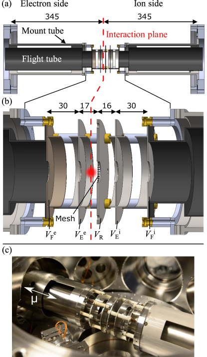
Figure 1: Drawing of the double velocity map imaging spectrometer (VMIS) (a) and an expanded view of the electrode package (b); dimensions are in mm. The indicated voltages are applied to the electron side flight tube ($V_{\mathrm{F}}^{\mathrm{e}}$), the electron side extractor ($V_{\mathrm{E}}^{\mathrm{e}}$), the repeller ($V_{\mathrm{R}}$), the ion side extractor ($V_{\mathrm{E}}^{\mathrm{i}}$) and the ion side flight tube ($V_{\mathrm{F}}^{\mathrm{i}}$). A photo of the spectrometer mounted in the experimental chamber is shown in (c). The sliding $\mu$-metal shield is marked by the letter $\mu$.

By changing $\eta$, the curvature of the field in the interaction region is changed, allowing for different imaging modes. Velocity map imaging mode is usually achieved for $\eta\approx 0.75$, with the exact value depending on the specific design geometry Eppink and Parker (1997). In this mode, electrons (or ions) with the same momentum in the plane parallel to the detection plane will be projected onto the same spot on the detector even if they are generated at different positions in the interaction region.

The full three-dimensional momentum distribution can be obtained through inversion procedures, as long as there is an axis of cylindrical symmetry in the ionization process Smith et al. (1988); Vrakking (2001). Another mode of operation, often referred to as the spatial imaging mode, is achieved for $\eta\approx 1$ Johnsson et al. (2010). The particle impact position on the detector is then most sensitive to where the charged particle is created, and therefore, the interaction region can be imaged. This is a useful mode for alignment purposes, providing a means of ensuring precise positioning of the XUV light focal spot, as well as good overlap between the laser beam and the molecular beam Johnsson et al. (2010). Moreover, by choosing $\eta$ between 0.78 and 0.8, a Wiley–McLaren ion time-of-flight mode can be achieved Wiley and McLaren (1955).

2.1 Design

The design of the double VMIS was made with the following goals: First, we wanted to add the capability to detect positively-charged ions without compromising the resolution on the electron side as compared to a standard VMIS. Second, as molecules have a typical ionization potential of 7–15 eV and, with HHG, the typical photon energies are up to 100 eV, the spectrometer should be able to focus electrons with energies up to $\approx$90 eV and ions with kinetic energies up to $\approx$10 eV, typical for, e.g., Coulomb explosion. Third, the spectrometer had to be compatible with the existing experimental chamber of the high-intensity XUV beamline at the Lund Attosecond Science Center containing the all-reflective short focal length XUV focusing optics Manschwetus et al. (2016); Coudert-Alteirac et al. (2017).

Extending the single-sided spectrometer to be able to record positively-charged ions and electrons simultaneously was the aim of this work. To that end, the design of the electron side, adapted from [44], was retained and the repeller electrode replaced by an electrode with a mesh, as shown in Figure 1b. On the ion side, an open extractor electrode and a flight tube, similar to that on the electron side, were added. There are two advantages with this choice of design. First, we are not changing the imaging conditions on the electron side, and second, once the optimum voltages have been found for the electrons, the voltages on the ion side can be tuned independently without affecting the electron image quality. The drawbacks are that the ions are to some extent scattered by the mesh, which has a transmission of $\sim$80%, and that they pass through a drift region before they pass the repeller and are focused by the fields on the ion side. This affects the energy resolution that can be achieved for the ion imaging, which will be discussed in Section 2.3.

The maximum electron or ion energy is restricted by the fact that the electrons or ions move away from the detector axis due to their initial velocity perpendicular to it. To increase the maximum detectable energy, one needs to either decrease the flight tube length, increase the flight tube and detector diameters or use higher acceleration voltages. In our case, the maximum detector size and the flight tube diameters were set by the existing chamber to $\sim$100 mm, leading to the choice of a standard MCP detector with a diameter of 75 mm, mounted on a CF160 flange. Similarly, the minimum flight tube lengths were set by the flange-to-flange distance (690 mm) of the existing experimental chamber to 345 mm. In principle, shorter flight tube lengths could have been achieved by a design where the MCPs are mounted inside the vacuum chamber, but this would have led to a more complicated design and a deteriorated TOF resolution, and was thus avoided.

With restrictions imposed on the detector size and flight tube length, the ratio between the maximum detectable kinetic energy and the acceleration voltage scales approximately as $\left(r/L\right)^{2}$, where $r$ is the detector radius and $L$ is the flight tube length. Under the chosen conditions, this means that particles with kinetic energies up to $\approx$1% of the acceleration voltage can be detected, meaning that a total voltage difference of almost 10 kV between the front of the electron MCP and the front of the ion MCP is required to detect electrons and ions with 90 eV and 10 eV of kinetic energy, respectively.

The design of the assembly was made in such a way that both detectors, electrodes and flight tubes could be supplied with floating voltages of $\pm 10$ kV. While the front of the MCPs are not electrically connected to the flight tubes, for the following discussion and simulations, we assume that the same voltage is applied to the front of the MCP and the flight tube.

The resulting design of the double VMIS is shown in Figure 1 together with the relevant dimensions. The spectrometer is mounted horizontally, and the electron and ion sides are separable between the repeller electrode and the ion extractor electrode to facilitate mounting of the spectrometer on the two opposite CF200 flanges of the experimental chamber. The mounting flanges are CF200 to CF160 zero-length reducers, allowing for convenient mounting of the detectors after the spectrometer has been installed. In order to allow for floating voltages on the flight tubes, ceramic spacers are used between these and the supporting grounded mount tubes, which are made of stainless steel. While the ion flight tube is made of stainless steel, the electron flight tube is made of $\mu$-metal to provide shielding from external magnetic fields. In addition, a sliding $\mu$-metal cylinder with holes for the laser beam and the molecular beam, visible on the far left in Figure 1c, can be moved in to shield also the electrode assembly. The flight tubes have a front brim, which is supported by four rods via ceramic spacers (white parts in Panel (b)) and bushings (yellow parts in Panel (b)). These brims also hold the electrodes, which can be conveniently reached and exchanged from the top of the chamber without unmounting the flight tube assemblies. The electrodes are mounted with ceramic bushings (yellow parts in Panel (b)) on rods made out of Vespel^®, separated by ceramic spacers (white parts in Panel (b)). No electrode or grounded parts are closer than 10 mm apart to allow for large voltage differences without the risk of arcing.

The final design offers a large versatility by allowing for voltages of $\pm 10$ kV to be applied to any of the spectrometer components (electrodes or flight tubes), and the choice of a mesh in the repeller electrode allows for independent tuning of the ion sides without affecting the electron imaging. The physical design makes it easy to mount and dismount the whole or parts of the spectrometer, and while being dimensioned for use in the existing experimental chamber, the assembly can be easily transferred also to chambers with other geometries.

2.2 Operation Modes

The spectrometer can be operated in different photo-electron and -ion detection modes. A selection of spectroscopically-relevant modes is listed below:

1. High resolution ion modes:

   1. Ion TOF,

   2. Ion VMI.

2. High resolution electron modes:

   1. Electron VMI, ion TOF,

   2. Electron VMI, ion VMI.

In the high resolution ion modes, the voltages are set to accelerate and detect ions on the electron side, as a standard single-side VMI, either in TOF mode (1(a)) under Wiley-McLaren conditions Wiley and McLaren (1955) or in VMI mode (1(b)). With this setting, the mesh in the repeller electrode does not impose any restriction on the achievable mass or energy resolution, since the ion side of the spectrometer is not used (see Figure 1). In the high resolution electron modes, the electron side of the spectrometer is configured for optimum VMI conditions for electrons, while the ion side voltages are set either for ion TOF (2(a)) or ion VMI (2(b)). The different modes are explored in Section 2.3.

2.3 Simulations

To evaluate the expected performance of the spectrometer, simulations were carried out using SIMION Dahl (2000) for the different operation modes listed above. An interaction region, defined by the overlap between the laser beam and the molecular beam, with a conservatively chosen size of $(100~{}\times 100\times 2000)$ $\upmu$m³ was used. For the VMI calculations, electron kinetic energies were chosen in steps of 5 eV from 10–90 eV and ion kinetic energies in steps of 1 eV from 2 to 10 eV. For each operation mode, we found optimum voltages, defined as the voltages for which the best resolution is obtained for electrons with a kinetic energy of 30 eV and singly-charged ions with a kinetic energy of 6 eV and a mass of $m=100$ u. The kinetic energies were chosen based on the typical energies of the photoelectrons and photoions of interest using high-order harmonics generated in argon to ionize molecules with ionization potentials in the 10–20-eV range, and the mass was chosen because it is typical for systems that are of current scientific interest, like small polycyclic aromatic hydrocarbons.

To find the optimum voltages for the VMI modes, a simplified simulation procedure was used, in which the trajectories of 27 particles arranged on a $3\times 3\times 3$ grid covering the interaction region and with their velocity component perpendicular to the detector axis were calculated and the energy or mass resolution calculated from the particle impact position distribution on the detector. For the optimum voltages found (summarized in Table 1), a procedure based on Monte Carlo sampling was used Ghafur et al. (2009), resulting in more realistic resolution estimates. The method consisted of launching a large number of electrons or ions ($\sim$10⁶) with a random starting position chosen from a Gaussian distribution over the interaction volume and with a random, isotropically-distributed 3D initial momentum. The particle impacts on the detector were then sampled to generate a simulated detector image or TOF trace, which was treated similarly to experimental data in order to extract the resolution. The simulated images were inverted using an iterative algorithm Vrakking (2001) to retrieve the 3D momentum distribution from the 2D image. From the 3D momentum distribution, the energy spectrum was calculated, and the energy resolution, $\Delta E/E$, was estimated by obtaining $\Delta E$ from the full width at half maximum of a Gaussian fit to the peaks in the spectrum. For the TOF simulations, only the Monte Carlo method was used, and the mass resolution, $m/\Delta m$, was calculated by obtaining $\Delta m$ from the full width at half maximum of a Gaussian fit to the peaks in the mass spectrum. They were performed both for ions with zero kinetic energy and for ions with an initial velocity in the direction of the molecular beam. The latter represents the more realistic scenario of target molecules with a mass of 100 u that are brought into the interaction region by a carrier gas, e.g., helium. This carrier gas typically travels at a speed of 1000 m/s, which corresponds to a kinetic energy of 520 meV for molecules with a mass of 100 u.

Operation Mode	$\eta$ (Equation (1))	$V_{\text{F}}^{\text{e}}$ (kV)	$V_{\text{E}}^{\text{e}}$ (kV)	$V_{\text{R}}$ (kV)	$V_{\text{E}}^{\text{i}}$ (kV)	$V_{\text{F}}^{\text{i}}$ (kV)
1(a) Ion TOF	0.76–0.78	0	2.275–2.354	3.000	not used	not used
1(b) Ion VMI	0.76	0	2.275	3.000	not used	not used
2(a) Electron VMI + ion TOF	0.76	5.000	$-$5.775	$-$9.200	$-$10.000	$-$10.000
2(b) Electron VMI + ion VMI	0.76	5.000	$-$5.775	$-$9.200	$-$8.802	$-$10.000

Table 1: Simulated optimum voltages for the different operation modes. For Mode 1(a), the exact optimum voltage $V_{\text{E}}^{\text{e}}$ depends on the initial velocity of the ions.

2.3.1 High Resolution Ion Modes

For the high resolution ion modes, ions are detected on the electron side of the spectrometer, and for the simulations, the choice was made to ground the front of the MCP and the flight tube ($V_{\mathrm{F}}^{\mathrm{e}}=0$ kV). The repeller voltage was set to $V_{\mathrm{R}}=3$ kV. Figure 2a shows the resulting mass resolution in Operation Mode 1(a) for extractor voltages from 1400–3000 V. For zero kinetic energy ions, the optimum extractor voltage was found to be $V_{\mathrm{E}}^{\mathrm{e}}=2.354$ kV ($\eta=0.78$, black curve). The resolution of $m/\Delta m=$ 35,000 is clearly over-estimated, and for the more realistic case of ions with an initial drift velocity, the best resolution of $m/\Delta m=2000$ was found for a voltage of $V_{\mathrm{E}}^{\mathrm{e}}=2.275$ kV ($\eta=0.76$, blue curve).

Figure 2b shows the resulting energy resolution for ion VMI in Operation Mode 1(b) for three different settings for the extractor voltage, $V_{\mathrm{E}}^{\mathrm{e}}$, calculated using the 27-particle model (blue, green and orange lines). The optimum extractor voltage, for which the best resolution was achieved for a photoion kinetic energy of 6 eV, was found to be $V_{\mathrm{E}}^{\mathrm{e}}=2.275$ kV ($\eta=0.76$), and for this setting, the resulting energy resolution from the Monte Carlo simulation is shown (black line), indicating an energy resolution better than $1.5\%$ for kinetic energies between 6 and 10 eV. In Figure 2c,d, the corresponding simulated detector image and the 3D momentum distribution after inversion are shown, respectively. Figure 2e shows the kinetic energy spectrum calculated from the 3D momentum distribution.

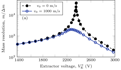
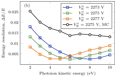
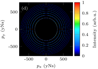
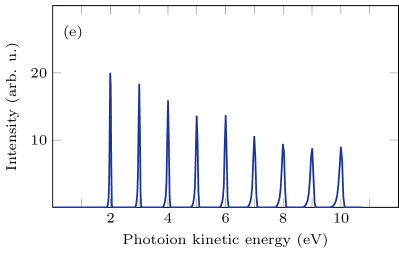
Figure 2: Simulation results for the high resolution ion modes. (a) shows the resulting mass resolution at mass $m=100$ u as a function of extractor voltage, $V_{\mathrm{E}}^{\mathrm{e}}$, for ions with zero initial kinetic energy (black) and ions with an initial velocity of $v_{0}=1000$ m/s in the direction of the molecular beam (blue). (b) shows the resulting VMI energy resolution for three different extractor voltages ($V_{\mathrm{E}}^{\mathrm{e}}$) using the 27-particle model (blue, green and orange lines) and the Monte Carlo model for the optimum setting (black line). (c,d) show the simulated detector image and the 3D momentum distribution after inversion, for the optimum voltages. (e) shows the kinetic energy spectrum calculated from the 3D momentum distribution.

2.3.2 High Resolution Electron Modes

For the high resolution electron modes, electrons and ions are detected on their respective sides of the spectrometer. To maximize the possible total voltage difference over the spectrometer, the voltage on the electron side flight tube (and thus, the front of the electron MCP) was set to $V_{\mathrm{F}}^{\mathrm{e}}=5$ kV, so that the phosphor screen could still be operated at its full voltage bias of 5 kV relative to the front of the MCP without exceeding the limit of the electrical feedthroughs. The repeller voltage was set to $V_{\mathrm{R}}=-9.2$ kV to allow for detection of electrons with kinetic energies up to 90 eV, while allowing for extraction and imaging of ions with kinetic energies up to 10 eV.

Figure 3a shows the resulting energy resolution for electron VMI for three different settings for the extractor voltage, $V_{\mathrm{E}}^{\mathrm{e}}$, calculated using the 27-particle model (blue, green and orange lines). The optimum extractor voltage, for which the best resolution was achieved for a photoelectron energy of 30 eV, was found to be $V_{\mathrm{E}}^{\mathrm{e}}=-5.775$ kV ($\eta=0.76$), and for this setting, the resulting energy resolution from the Monte Carlo simulation is shown (black line), indicating an energy resolution better than $2\%$ for photoelectron energies between 30 and 85 eV. In Figure 3b,c, the corresponding simulated detector image and the 3D momentum distribution after inversion are shown, respectively. Figure 3d shows the photoelectron energy spectrum calculated from the 3D momentum distribution.

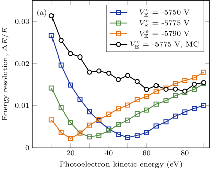
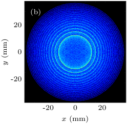
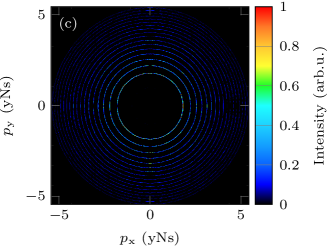
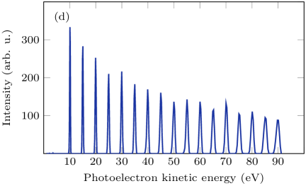
Figure 3: Simulation results for high resolution electron VMI mode. (a) shows the resulting energy resolution for three different extractor voltages ($V_{\mathrm{E}}^{\mathrm{e}}$) using the 27-particle model (blue, green and orange lines) and the Monte Carlo model for the optimum setting (black line). (b,c) show the simulated detector image and the 3D momentum distribution after inversion, for the optimum voltages. (d) shows the photoelectron energy spectrum calculated from the 3D momentum distribution.

With the electron side conditions optimized for electron VMI and the voltage on the ion side flight tube set to $V_{\mathrm{F}}^{\mathrm{i}}=-10$ kV to detect ions with kinetic energies up to 10 eV, the ion side can be tuned either for TOF (Operation Mode 2(a)) or VMI (Operation Mode 2(b)) by varying the ion extractor electrode voltage, $V_{\mathrm{E}}^{\mathrm{i}}$.

Figure 5a shows the resulting mass resolution in Operation Mode 2(a) for ions with an initial velocity of 1000 m/s in the direction of the molecular beam, for different extractor voltages, $V_{\mathrm{E}}^{\mathrm{i}}$. It is clear that it is not possible to reach Wiley–McLaren conditions within the voltage limits of the setup, due to the initial drift region between the interaction point and the mesh through which the ions have to travel. In addition, the best mass resolution of $m/\Delta m=110$, achieved for $V_{\mathrm{E}}^{\mathrm{i}}=-10$ kV, is a factor of 18 worse than that achieved in Operation Mode 1(a). In fact, the mass resolution is in this case limited by the influence of the drift region and not by the initial velocity of the ions, and the mass resolution for zero kinetic energy ions (not shown) coincides with the mass resolution shown in Figure 5a. Figure 5b shows the resulting energy resolution for ion VMI in Operation Mode 2(b) for three different settings for the extractor voltage, $V_{\mathrm{E}}^{\mathrm{i}}$, calculated using the 27-particle model (blue, green and orange lines). The optimum extractor voltage, for which the best resolution was achieved for a kinetic energy of 6 eV, was found to be $V_{\mathrm{E}}^{\mathrm{i}}=-8.802$ kV, and for this setting, the resulting energy resolution from the Monte Carlo simulation is shown (black line), indicating an energy resolution better than $2.5\%$ for kinetic energies between 3 and 10 eV. This is a small degradation in resolution as compared to the resolution obtained in Operation Mode 1(b) (shown by the dashed black line), but it is still an acceptable resolution for ions in most experiments. It is interesting to note that even in Operation Mode 2(b), for $V_{\mathrm{E}}^{\mathrm{i}}=-8.802$ kV, the mass resolution of the ion TOF is $m/\Delta m=100$, which is acceptable unless isotope resolution of heavier fragments is required. In Figure 5c,d, the corresponding simulated detector image and the 3D momentum distribution after inversion are shown, respectively. Figure 5e shows the kinetic energy spectrum calculated from the 3D momentum distribution.

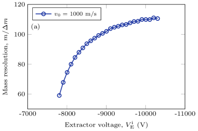
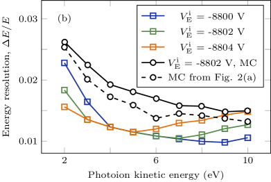
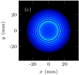
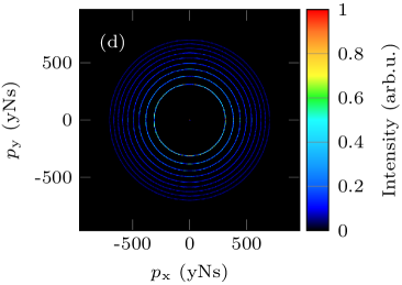
Figure 4: Cont.

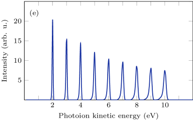
Figure 5: Simulation results for ion detection when the electron side is optimized for electron VMI (Operation Modes 2(a) and 2(b)). (a) shows the resulting mass resolution as a function of extractor voltage, $V_{\mathrm{E}}^{\mathrm{i}}$, for ions with an initial velocity of $v_{0}=1000$ m/s in the direction of the molecular beam. (b) shows the resulting VMI energy resolution for three different extractor voltages using the 27-particle model (blue, green and orange lines) and the Monte Carlo model for the optimum setting (solid black line). The dashed black line shows the resolution in Operation Mode 1(b) obtained by the Monte Carlo method, reproduced from Figure 2. (c,d) show the simulated detector image and the 3D momentum distribution after inversion, for the optimum voltages. (e) shows the kinetic energy spectrum calculated from the 3D momentum distribution.

3 Experimental Results

To evaluate the performance of the instrument, measurements have been done at the high-intensity XUV beamline at the Lund Attosecond Science Center Manschwetus et al. (2016), where high-flux XUV pulses generated through the HHG process were focused by reflective optics into the interaction region of the double VMIS. The target gas was introduced using a pulsed molecular beam from an Even–Lavie solenoid valve, able to produce high density pulses with durations as short as 10 $\upmu$s Even (2014, 2015). In Figure 6, the spectrum of the XUV pulses generated in argon and recorded by an XUV spectrometer is displayed. It contains photons from harmonic order 13 (20.0 eV) up to harmonic order 29 (44.7 eV). Lower photon energy contributions and the remaining driving laser light are absorbed by a 200 nm-thick aluminum filter. The XUV light is redirected to the XUV spectrometer by a rotatable gold mirror prior to the focusing into the interaction region of the double VMIS, and thus, the spectrum cannot be recorded during measurements with the double VMIS. The displayed XUV spectrum has been corrected for the spectral responses of the employed grating and MCP detector. In the further analysis, the corrected spectrum is used.

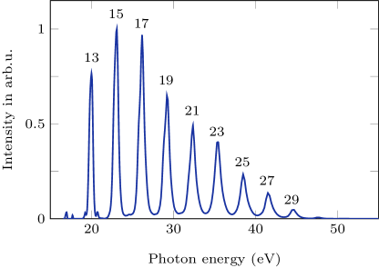
Figure 6: XUV spectrum recorded by the XUV spectrometer. The spectrum contains photons from harmonic order 13 (20.0 eV) up to harmonic order 29 (44.7 eV), indicated above the peaks.

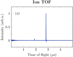
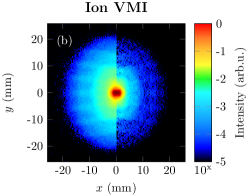
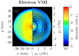
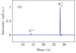
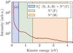
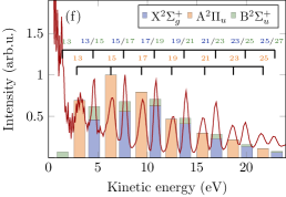
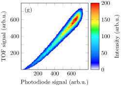
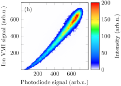
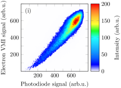
Figure 7: Experimental results in the high resolution electron mode (2(b)) using high-order harmonics generated in argon to ionize N₂. (a,d,g) show ion TOF data (a), with the calibrated mass spectrum in (d) and the correlation between the total ion TOF signal and the XUV intensity measured by the XUV photodiode visualized by a color-coded scatter plot in (g). (b,e,h) show ion VMI data, with the average detector image (left part) and inverted image (right part) in (b). The inverted images represent the reconstructed initial 3D momentum distributions obtained by inversion of the 2D projections recorded on the detector Vrakking (2001). The photoion kinetic energy spectrum is displayed in (e) with its attributed contributions shaded in different colors, calculated from the inverted image (b). The correlation between the total ion VMI signal and the XUV intensity is exhibited in (h). (c,f,i) show electron VMI data, with the average detector image (left part) and inverted image (right part) in (c). The photoelectron kinetic energy spectrum is displayed in panel (f) with the attributed electronic molecular channels and the color-coded corresponding harmonic orders. The correlation between the total electron VMI signal and the XUV intensity is shown in (i). The slight bend observed for low intensities in the correlation plots is likely caused by a non-linear behavior of the photodiode in this signal region.

To be able to apply covariance analysis, synchronized single-shot data need to be acquired. At the high-intensity XUV beamline, the repetition rate is 10 Hz, and acquisition of single-shot data is relatively straightforward. However, the intensity of the XUV light generated by laser-driven HHG typically varies on a shot-to-shot basis, introducing false correlations between channels that are physically not correlated. To circumvent this problem, a partial covariance method was used Frasinski et al. (1996), through which the covariance maps were corrected for the fluctuating source intensity, recorded on a single-shot basis by an in-vacuum XUV photodiode placed after the focus of the XUV pulses. In this section, we describe the acquisition of data and the subsequent proof-of-principle application of ion-ion and ion-electron covariance mapping.

3.1 Data Acquisition

The successful implementation of the partial covariance analysis technique, discussed above, requires that the different single-shot observables can be reliably recorded in a synchronized fashion. In order to achieve this, a timestamp server was set up. After receiving the trigger from the laser master clock, the acquisition programs signal their readiness to the server. If all programs signal within a set timeout, the server responds with a timestamp. Otherwise, it orders the programs to cancel the acquisition and to wait for the next trigger pulse. Typically, about 5% of the shots are discarded by the server. To fully evaluate the performance of the instrument, the acquisition of four synchronized signals is required:

• Ion time-of-flight trace

• Ion velocity map image

• Electron velocity map image

• XUV intensity from photodiode

The ion TOF trace was obtained by decoupling the current from the back of the ion MCP and converting it into a voltage signal. The XUV photodiode generates a current, which is converted to a voltage signal by means of a transimpedance amplifier. These analog ion TOF and XUV photodiode voltage traces are subsequently converted into digital signals using a two-channel, 1-GHz sampling rate, analog-to-digital converter (Agilent Acquiris DP1400), which acquires 20,000 samples per laser shot in each of the channels, with a dynamic range of eight bits. The ion and electron VMI data are recorded with two one-megapixel Allied Vision Technology Pike F-145B cameras that have an 8 bit dynamic range and a maximum frame rate of 30 Hz. In terms of storage rate, this amounts to more than 2 MB of data per shot, or 20 MB/s.

As a benchmark molecule, we used N₂. Figure 7 shows simultaneously-acquired data from N₂, acquired using voltage ratios corresponding to Operation Mode 2(b), i.e., optimized for electron and ion VMI, but with absolute voltages adapted for a maximum electron kinetic energy of 30 eV. The data were recorded for 25,000 laser shots, corresponding to just above 40 minutes of acquisition time and amounting to $\sim$50 GB of data. The molecules were ionized using the harmonics 13–29 generated in argon, corresponding to photon energies between 20 and 45 eV, as displayed in Figure 6. The typical on-target pulse energy was $\sim$5 nJ, which corresponds to approximately 10⁹ photons per pulse over the whole bandwidth and 10⁸ photons per pulse and harmonic. The count rates were on the order of 500 particles detected per shot for the ions, as well as the electrons.

Considering that the maximum available photon energy is just above the double ionization threshold of N₂ (42.88 eV Hochlaf et al. (1996)), a number of electronic states in N₂ with ionization potential (IP) in the range can be accessed: X${}^{2}\Sigma_{g}^{+}$, A${}^{2}\Pi_{u}$, B${}^{2}\Sigma_{u}^{+}$, C${}^{2}\Sigma_{u}^{+}$, F${}^{2}\Sigma_{g}^{+}$ and H${}^{2}\Sigma_{g}^{+}$. The average ion mass spectrum in Figure 7d exhibits two main features, which were assigned to the N⁺ and N${}_{2}^{+}$ channels. While the former also contains a contribution coming from stable N${}_{2}^{2+}$ ions, only photons from the 29th harmonic or higher can contribute, and considering the low intensity at these photon energies (Figure 6), the contribution from this channel is expected to be negligible. The mass resolution was estimated to $m/\Delta m=60$ for a mass of 28 u.

Figure 7b shows the photoion momentum distribution of all the ionic fragments that were generated in the interaction region, averaged over 25,000 shots. The anisotropy of the distribution, peaked in the vertical direction, is due to the fact that the cross-section for excitation to the dissociative states is higher for molecules aligned along the laser polarization direction. The faint horizontal ripple pattern in the images is a result of ions scattering on the mesh in the repeller electrode. In Figure 7e, the corresponding photoion kinetic energy is displayed. It reveals three main features: a peaked contribution shaded in blue, a broader feature shaded in green and another broad contribution almost spreading out to the edge of the detector shaded in orange. We attribute the strongest feature (shaded blue) to low kinetic energy N${}_{2}^{+}$ ions and predissociation of the N${}_{2}^{+}$ C${}^{2}\Sigma_{u}^{+}$ state Lucchini et al. (2012). The contribution shaded in green has previously been assigned to dissociation from the F${}^{2}\Sigma_{g}^{+}$ state, and the features in the area shaded in orange are associated with dissociation from the highly-excited Rydberg-like states of N${}_{2}^{+}$ and the H band Eckstein et al. (2015); Lucchini et al. (2012); Aoto and Ito (2006).

Figure 7c,f shows the photoelectron momentum distribution and the photoelectron kinetic energy spectrum, respectively. From the photoelectron spectrum, it is apparent that the resolution of the spectrometer is limited by the bandwidth of the harmonics ($\sim$0.5 eV) rather than by the electron imaging. Figure 7f contains the assigned contributions originating from the X${}^{2}\Sigma_{g}^{+}$, A${}^{2}\Pi_{u}$ and B${}^{2}\Sigma_{u}^{+}$ states, after taking their respective branching ratios, cross-sections Plummer et al. (1977); Hammet et al. (1976) and the relative XUV intensity at the photon energies contained in the XUV spectrum into account. The ratio of the contributions is displayed by a stacked bar plot, where each state has a specific color assigned. The much weaker contributions of the other cationic and dicationic states are not shown for clarity Aoto and Ito (2006); Plummer et al. (1977); Baltzer et al. (1992); Ahmad et al. (2006). The signal at kinetic energies smaller than 1 eV can be assigned to highly excited inner valence states of N${}_{2}^{+}$ and possibly the first electronic states of N${}_{2}^{2+}$ Eckstein et al. (2015); Aoto and Ito (2006); Ahmad et al. (2006).

As mentioned earlier, in order to extract information about the correlation between the different single-shot datasets, it is important that the sets are acquired simultaneously and can be analyzed in a synchronized fashion. That this is indeed the case for the acquired dataset readily verified by studying the color-coded scatter plots in Figure 7g–i, indicating a high degree of correlation between the XUV intensity measured by the photodiode and the other three detector signals.

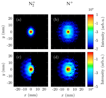
Figure 8: Results of ion-ion covariance analysis. (a,b) show covariance maps of the N${}_{2}^{+}$ and the N⁺ ion TOF fragments correlated with the ion VMI detector image, respectively. Furthermore, these maps were treated like raw VMI images and inverted. The results are displayed in the right halves of (c,d). For comparison the inverted image of the accumulated ion detector image from Figure 7b is reproduced in the left halves.

3.2 Covariance Analysis

Once the synchronized acquisition of data from all the detectors is established, covariance analysis can be applied to different variables to reveal more information about the underlying physical processes during and after the photoionization. As a proof-of-principle demonstration, we use covariance mapping to achieve post-acquisition mass selection of different ionic species. The aim is to extract the momentum distributions for individual ionic species from the average momentum distribution Figure 7b by calculating the covariance image with respect to the corresponding peak in the ion TOF spectrum shown in Figure 7a. For mass selection, temporal windows around the two features in the time-of-flight spectrum in Figure 7a were chosen. For this, the partial covariance Frasinski et al. (1996), $\text{pcov}(\mathbf{X},\mathbf{Y})$, between every pixel in the ion velocity map image ($\mathbf{X}$) with the total signal in the studied channel in the time-of-flight spectrum ($\mathbf{Y}$) was calculated.

The resulting covariance maps are displayed in Figure 8a for the N${}_{2}^{+}$ channel and in Figure 8b for the N⁺ channel. As expected, the N${}_{2}^{+}$ map (a) is dominated by the zero kinetic energy parent ions from ionization to the X${}^{2}\Sigma_{g}^{+}$, A${}^{2}\Pi_{u}$ and B${}^{2}\Sigma_{u}^{+}$ states. The N⁺ map (b) shows correlation both at low kinetic energies, previously attributed to the predissociation of the N${}_{2}^{+}$ C${}^{2}\Sigma_{u}^{+}$ state and, at higher kinetic energies, previously attributed to dissociation from the F${}^{2}\Sigma_{g}^{+}$ state, highly excited Rydberg-like states of N${}_{2}^{+}$ and the H band. Further, in order to compare it to the accumulated ion VMI data, the same inversion procedure was applied to the covariance maps. The results are shown side by side with the reproduced inverted data from Figure 7b in the left halves of Figure 8c for N${}_{2}^{+}$ and Figure 8d for N⁺, with the right halves being the inverted covariance maps. These results clearly show that mass selection via covariance is a viable method to extract correlated information about the products of photoionization using the proposed instrument.

A natural next step is to consider ion-electron covariance using this scheme. Consequently, the photoelectron covariance maps were calculated in an analogous way to the ion covariance maps shown in Figure 8a,b. Due to insufficient statistics, it was not possible to adequately invert the resulting covariance maps, and instead, the results of an angular integration of these are shown in Figure 9. Since, as shown in Figure 7f, the photoelectron spectrum primarily contains electrons from the X${}^{2}\Sigma_{g}^{+}$, A${}^{2}\Pi_{u}$ and B${}^{2}\Sigma_{u}^{+}$ states that are all coupled to the N${}_{2}^{+}$ channel, these completely dominate the covariance at photoelectron momenta between 1 and 2.6 yNs. While the individual peaks cannot be clearly resolved, partly due to a downsampling of the data for reasons of statistics, the contribution is stronger for the N${}_{2}^{+}$ channel in this regime, as expected. However, at close to zero momentum, the contribution associated with the production of N⁺ from dissociation is dominating, which is consistent with our previous attribution of these low kinetic energy electrons to excitation of inner valence states of N${}_{2}^{+}$. Although qualitative, these first ion-electron covariance results indicate the feasibility of using covariance analysis to extract channel-specific photoelectron data from experiments with high single-shot count rates using the double VMIS presented here.

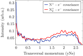
Figure 9: Results of ion-electron covariance analysis. Covariance between the photoelectron transversal momentum spectrum and the ion-TOF channels of N⁺ (blue) and N${}_{2}^{+}$ (red). Qualitatively, the N⁺ channel shows stronger correlation with low momentum photoelectrons, whereas the N${}_{2}^{+}$ channel exhibits a stronger correlation with photoelectrons at higher transversal momenta.

4 Conclusions and Outlook

In conclusion, we have reported on the design and performance of a velocity map imaging (VMI) spectrometer optimized for experiments using high-intensity extreme ultraviolet (XUV) sources such as laser-driven high-order harmonic generation (HHG) sources and free-electron lasers (FELs). The instrument is versatile and allows for combining photo-electron and -ion detection modes, such as ion time-of-flight (TOF), ion VMI and electron VMI, in different ways, depending on the required information and the process under study. The performance for the different detection modes was estimated using simulations, and first experimental results from an intense HHG source were presented together with proof-of-principle application of covariance mapping to mass selection of photoions and extraction of channel-specific photoelectron spectra.

The analysis of the experimental results confirms that the acquired data contain information about the correlation between the products of the photoionization, and the first covariance mapping analysis demonstrates the feasibility of extracting such information, indicating that the suggested approach is viable for extracting feature-rich correlated information from future experiments using high-intensity XUV sources.

Conceptualization: L.R. and P.J. Data curation: L.R., J.L. and S.M. Formal analysis: L.R., J.L., S.M. and P.J. Funding acquisition: P.J. Investigation: L.R., J.L., S.M., F.C., H.C.-A., B.O., J.P., H.W., P.R. and M.G. Project administration: P.J. Supervision: P.J.; Writing, original draft: L.R. and J.L. Writing, review and editing: L.R., J.L., S.M., F.C., H.C.-A., B.O., J.P., H.W., P.R., M.G. and P.J.

This research was supported by the Swedish Research Council, the Swedish Foundation for Strategic Research and the Crafoord Foundation. This project has received funding from the European Union’s Horizon 2020 research and innovation program under the Marie Sklodowska-Curie Grant Agreement No. 641789 MEDEA.

The authors declare no conflict of interest. The founding sponsors had no role in the design of the study; in the collection, analyses or interpretation of data; in the writing of the manuscript; nor in the decision to publish the results.

References

References

- Ferray et al. (1988) Ferray, M.; L’Huillier, A.; Li, X.; Lompre, L.; Mainfray, G.; Manus, C. Multiple-harmonic conversion of 1064 nm radiation in rare gases. J. Phys. B 1988, 21, L31.
- Agostini and DiMauro (2004) Agostini, P.; DiMauro, L.F. The physics of attosecond light pulses. Rep. Prog. Phys 2004, 67, 813.
- McPherson et al. (1987) McPherson, A.; Gibson, G.; Jara, H.; Johann, U.; Luk, T.S.; McIntyre, I.A.; Boyer, K.; Rhodes, C.K. Studies of multiphoton production of vacuum-ultraviolet radiation in the rare gases. J. Opt. Soc. Am. B 1987, 4, 595–601.
- Corkum (1993) Corkum, P. Plasma perspective on strong-field multiphoton ionization. Phys. Rev. Lett. 1993, 71, 1994.
- Schafer et al. (1993) Schafer, K.J.; Yang, B.; DiMauro, L.F.; Kulander, K.C. Above threshold ionization beyond the high harmonic cutoff. Phys. Rev. Lett. 1993, 70, 1599.
- Ackermann et al. (2007) Ackermann, W.A.; Asova, G.; Ayvazyan, V.; Azima, A.; Baboi, N.; Bähr, J.; Balandin, V.; Beutner, B.; Brandt, A.; Bolzmann, A.; et al. Operation of a free-electron laser from the extreme ultraviolet to the water window. Nat. Photonics 2007, 1, 336.
- Emma et al. (2010) Emma, P.; Akre, R.; Arthur, J.; Bionta, R.; Bostedt, C.; Bozek, J.; Brachmann, A.; Bucksbaum, P.; Coffee, R.; Decker, F.J.; et al. First lasing and operation of an ångstrom-wavelength free-electron laser. Nat. Photonics 2010, 4, 641.
- Ishikawa et al. (2012) Ishikawa, T.; Aoyagi, H.; Asaka, T.; Asano, Y.; Azumi, N.; Bizen, T.; Ego, H.; Fukami, K.; Fukui, T.; Furukawa, Y.; et al. A compact X-ray free-electron laser emitting in the sub-ångström region. Nat. Photonics 2012, 6, 540.
- McNeil and Thompson (2010) McNeil, B.W.J.; Thompson, N.R. X-ray free-electron lasers. Nat. Photonics 2010, 4, 814.
- Glownia et al. (2010) Glownia, J.M.; Cryan, J.; Andreasson, J.; Belkacem, A.; Berrah, N.; Blaga, C.I.; Bostedt, C.; Bozek, J.; DiMauro, L.F.; Fang, L.; et al. Time-resolved pump-probe experiments at the LCLS. Opt. Express 2010, 18, 17620–17630.
- Lépine et al. (2014) Lépine, F.; Ivanov, M.Y.; Vrakking, M.J.J. Attosecond molecular dynamics: Fact or fiction? Nat. Photonics 2014, 8, 195.
- Krausz and Ivanov (2009) Krausz, F.; Ivanov, M. Attosecond physics. Rev. Mod. Phys. 2009, 81, 163–234.
- Sorokin et al. (2007) Sorokin, A.; Wellhöfer, M.; Bobashev, S.; Tiedtke, K.; Richter, M. X-ray-laser interaction with matter and the role of multiphoton ionization: Free-electron-laser studies on neon and helium. Phys. Rev. A 2007, 75, 051402.
- Berrah et al. (2010) Berrah, N.; Bozek, J.; Costello, J.T.; Düsterer, S.; Fang, L.; Feldhaus, J.; Fukuzawa, H.; Hoener, M.; Jiang, Y.H.; Johnsson, P.; et al. Non-linear processes in the interaction of atoms and molecules with intense EUV and X-ray fields from SASE free electron lasers (FELs). J. Mod. Opt. 2010, 57, 1015–1040.
- Bucksbaum et al. (2011) Bucksbaum, P.H.; Coffee, R.; Berrah, N. The First Atomic and Molecular Experiments at the Linac Coherent Light Source X-Ray Free Electron Laser. In Advances in Atomic, Molecular, and Optical Physics; Academic Press: Cambridge, MA, USA, 2011; p. 239.
- Fang et al. (2012) Fang, L.; Osipov, T.; Murphy, B.; Tarantelli, F.; Kukk, E.; Cryan, J.P.; Glownia, M.; Bucksbaum, P.H.; Coffee, R.N.; Chen, M.; et al. Multiphoton Ionization as a clock to Reveal Molecular Dynamics with Intense Short X-ray Free Electron Laser Pulses. Phys. Rev. Lett. 2012, 109, 263001.
- Gallagher-Jones et al. (2014) Gallagher-Jones, M.; Bessho, Y.; Kim, S.; Park, J.; Kim, S.; Nam, D.; Kim, C.; Kim, Y.; Miyashita, O.; Tama, F.; et al. Macromolecular structures probed by combining single-shot free-electron laser diffraction with synchrotron coherent X-ray imaging. Nat. Commun. 2014, 5, 3798.
- Seibert et al. (2011) Seibert, M.M.; Ekeberg, T.; Maia, F.R.; Svenda, M.; Andreasson, J.; Jönsson, O.; Odić, D.; Iwan, B.; Rocker, A.; Westphal, D.; et al. Single mimivirus particles intercepted and imaged with an X-ray laser. Nature 2011, 470, 78–81.
- Neutze et al. (2000) Neutze, R.; Wouts, R.; Van der Spoel, D.; Weckert, E.; Hajdu, J. Potential for biomolecular imaging with femtosecond X-ray pulses. Nature 2000, 406, 752–757.
- Ullrich et al. (2003) Ullrich, J.; Moshammer, R.; Dorn, A.; Dörner, R.; Schmidt, L.P.H.; Schmidt-Böcking, H. Recoil-ion and electron momentum spectroscopy: Reaction-microscopes. Rep. Prog. Phys. 2003, 66, 1463–1545.
- Eppink and Parker (1997) Eppink, A.T.J.B.; Parker, D.H. Velocity map imaging of ions and electrons using electrostatic lenses: Application in photoelectron and photofragment ion imaging of molecular oxygen. Rev. Sci. Instrum. 1997, 68, 3477–3484.
- Smith et al. (1988) Smith, L.M.; Keefer, D.R.; Sudharsanan, S. Abel inversion using transform techniques. J. Quant. Spectrosc. Radiat. Transf. 1988, 39, 367–373.
- Vrakking (2001) Vrakking, M.J.J. An iterative procedure for the inversion of two-dimensional ion/photoelectron imaging experiments. Rev. Sci. Instrum. 2001, 72, 4084–4089.
- Eland (1978) Eland, J.H.D. Improved resolution in fixed-wavelength photoelectron–photoion coincidence spectroscopy. Rev. Sci. Instrum. 1978, 49, 1688–1690.
- Bodi et al. (2012) Bodi, A.; Hemberger, P.; Gerber, T.; Sztáray, B. A new double imaging velocity focusing coincidence experiment: i2PEPICO. Rev. Sci. Instrum. 2012, 83, 083105.
- Sztáray et al. (2017) Sztáray, B.; Voronova, K.; Torma, K.G.; Covert, K.J.; Bodi, A.; Hemberger, P.; Gerber, T.; Osborn, D.L. CRF-PEPICO: Double velocity map imaging photoelectron photoion coincidence spectroscopy for reaction kinetics studies. J. Chem. Phys. 2017, 147, 013944.
- Garcia et al. (2009) Garcia, G.A.; Soldi-Lose, H.; Nahon, L. A versatile electron-ion coincidence spectrometer for photoelectron momentum imaging and threshold spectroscopy on mass selected ions using synchrotron radiation. Rev. Sci. Instrum. 2009, 80, 023102.
- O’Keeffe et al. (2011) O’keeffe, P.; Bolognesi, P.; Coreno, M.; Moise, A.; Richter, R.; Cautero, G.; Stebel, L.; Sergo, R.; Pravica, L.; Ovcharenko, Y.; et al. Rev. Sci. Instrum. 2011, 82, 033109.
- Garcia and Nahon (2005) Garcia, G.A.; Nahon, L. A refocusing modified velocity map imaging electron/ion spectrometer adapted to synchrotron radiation studies. Rev. Sci. Instrum. 2005, 76, 053302.
- Frasinski et al. (1989) Frasinski, L.J.; Codling, K.; Hatherly, P.A. Covariance Mapping: A Correlation Method Applied to Multiphoton Multiple Ionization. Science 1989, 246, 1029–1031.
- Frasinski et al. (1992) Frasinski, L.J.; Stankiewicz, M.; Hatherly, P.A.; Cross, G.M.; Codling, K.; Langley, A.J.; Shaikh, W. Molecular H2 in intense laser fields probed by electron-electron, electron-ion, and ion-ion covariance techniques. Phys. Rev. A 1992, 46, R6789–R6792.
- Frasinski (2016) Frasinski, L.J. Covariance mapping techniques. J. Phys. B 2016, 49, 152004.
- Kornilov et al. (2013) Kornilov, O.; Eckstein, M.; Rosenblatt, M.; Schulz, C.P.; Motomura, K.; Rouzée, A.; Klei, J.; Foucar, L.; Siano, M.; Lübcke, A.; et al. Coulomb explosion of diatomic molecules in intense XUV fields mapped by partial covariance. J. Phys. B 2013, 46, 164028.
- Boguslavskiy et al. (2012) Boguslavskiy, A.E.; Mikosch, J.; Gijsbertsen, A.; Spanner, M.; Patchkovskii, S.; Gador, N.; Vrakking, M.J.J.; Stolow, A. The Multielectron Ionization Dynamics Underlying Attosecond Strong-Field Spectroscopies. Science 2012, 335, 1336–1340.
- Zhu and W. T. Hill (1997) Zhu, J.; W. T. Hill, I. Momentum and correlation spectra following intense-field dissociative ionization of H2. J. Opt. Soc. Am. B 1997, 14, 2212–2220.
- Hansen et al. (2012) Hansen, J.L.; Nielsen, J.H.; Madsen, C.B.; Lindhardt, A.T.; Johansson, M.P.; Skrydstrup, T.; Madsen, L.B.; Stapelfeldt, H. Control and femtosecond time-resolved imaging of torsion in a chiral molecule. J. Chem. Phys. 2012, 136, 204310.
- Slater et al. (2015) Slater, C.S.; Blake, S.; Brouard, M.; Lauer, A.; Vallance, C.; Bohun, C.S.; Christensen, L.; Nielsen, J.H.; Johansson, M.P.; Stapelfeldt, H. Coulomb-explosion imaging using a pixel-imaging mass-spectrometry camera. Phys. Rev. A 2015, 91, 053424.
- Pickering et al. (2016) Pickering, J.D.; Amini, K.; Brouard, M.; Burt, M.; Bush, I.J.; Christensen, L.; Lauer, A.; Nielsen, J.H.; Slater, C.S.; Stapelfeldt, H. Communication: Three-fold covariance imaging of laser-induced Coulomb explosions. J. Chem. Phys. 2016, 144, 161105, doi:10.1063/1.4947551.
- Osipov et al. (2018) Osipov, T.; Bostedt, C.; Castagna, J.C.; Ferguson, K.R.; Bucher, M.; Montero, S.C.; Swiggers, M.L.; Obaid, R.; Rolles, D.; et al. The LAMP instrument at the Linac Coherent Light Source free-electron laser. Rev. Sci. Instrum. 2018, 89, 035112.
- Johnsson et al. (2010) Johnsson, P.; Rouzée, A.; Siu, W.; Huismans, Y.; Lépine, F.; Marchenko, T.; Düsterer, S.; Tavella, F.; Stojanovic, N.; Redlin, H.; et al. Characterization of a two-color pump–probe setup at FLASH using a velocity map imaging spectrometer. Opt. Lett. 2010, 35, 4163–4165.
- Wiley and McLaren (1955) Wiley, W.C.; McLaren, I.H. Time-of-Flight Mass Spectrometer with Improved Resolution. Rev. Sci. Instrum. 1955, 26, 1150.
- Manschwetus et al. (2016) Manschwetus, B.; Rading, L.; Campi, F.; Maclot, S.; Coudert-Alteirac, H.; Lahl, J.; Wikmark, H.; Rudawski, P.; Heyl, C.M.; Farkas, B.; et al. Two-photon double ionization of neon using an intense attosecond pulse train. Phys. Rev. A 2016, 93, 061402.
- Coudert-Alteirac et al. (2017) Coudert-Alteirac, H.; Dacasa, H.; Campi, F.; Kueny, E.; Farkas, B.; Brunner, F.; Maclot, S.; Manschwetus, B.; Wikmark, H.; Lahl, J.; et al. Micro-Focusing of Broadband High-Order Harmonic Radiation by a Double Toroidal Mirror. Appl. Sci. 2017, 11, 1159.
- Rosca-Pruna (2001) Rosca-Pruna, F. Alignment of Diatomic Molecules Induced by Intense Laser Fields. Ph.D. Thesis, VU University of Amsterdam: Amsterdam, The Netherlands, 2001.
- Dahl (2000) Dahl, D.A. Simion for the personal computer in reflection. Int. J. Mass Spectrom. 2000, 200, 3–25.
- Ghafur et al. (2009) Ghafur, O.; Siu, W.; Johnsson, P.; Kling, M.F.; Drescher, M.; Vrakking, M.J.J. A velocity map imaging detector with an integrated gas injection system. Rev. Sci. Instrum. 2009, 80, 033110.
- Even (2014) Even, U. Pulsed Supersonic Beams from High Pressure Source: Simulation Results and Experimental Measurements. Adv. Chem. 2014, 2014, 1–11.
- Even (2015) Even, U. The Even-Lavie valve as a source for high intensity supersonic beam. EPJ Tech. Instrum. 2015, 2, 17.
- Frasinski et al. (1996) Frasinski, L.J.; Giles, A.; Hatherly, P.; Posthumus, J.; Thompson, M.; Codling, K. Covariance mapping and triple coincidence techniques applied to multielectron dissociative ionization. J. Electron Spectrosc. Relat. Phenom. 1996, 79, 367–371.
- Hochlaf et al. (1996) Hochlaf, M.; Hall, R.I.; Penent, F.; Kjeldsen, H.; Lablanquie, P.; Lavollée, M.; Eland, J.H.D. Threshold photoelectrons coincidence spectroscopy of N22+ and CO2+ ions. Chem. Phys. 1996, 207, 159–165.
- Lucchini et al. (2012) Lucchini, M.; Kim, K.; Calegari, F.; Kelkensberg, F.; Siu, W.; Sansone, G.; Vrakking, M.J.J.; Hochlaf, M.; Nisoli, M. Autoionization and ultrafast relaxation dynamics of highly excited states in N2. Phys. Rev. A 2012, 86, 043404.
- Eckstein et al. (2015) Eckstein, M.; Yang, C.H.; Kubin, M.; Frasetto, F.; Poletto, L.; Ritze, H.H.; Vrakking, M.J.J.; Kornilov, O. Dynamics of N2 Dissociation upon Inner-Valence Ionization by Wavelength-Selected XUV Pulses. J. Phys. Chem. Lett. 2015, 6, 419–425.
- Aoto and Ito (2006) Aoto, T.; Ito, K. Inner-valence states of N2+ and the dissociation dynamics studied by threshold photoelectron spectroscopy and configuration interaction calculation. J. Chem. Phys. 2006, 124, 234306.
- Plummer et al. (1977) Plummer, E.W.; Gustafsson, T.; Gudat, W.; Eastman, D.E. Partial photoionization cross sections of N2 and CO using synchrotron radiation. Phys. Rev. A 1977, 15, 2339–2355.
- Hammet et al. (1976) Hammet, A.; Stoll, W.; Brion, C. Photoelectron branching ratios and partial ionization cross-sections for CO and N2 in the energy range 18–50 eV. J. Electron Spectrosc. Relat. Phenom. 1976, 8, 367–376.
- Baltzer et al. (1992) Baltzer, P.; Larsson, M.; Karlsson, L.; Wannberg, B.; Carlsson-Göthe, M. Inner-valence states of N2+ studied by uv photoelectron spectroscopy and configuration-interaction calculations. Phys. Rev. A 1992, 46, 5545–5553.
- Ahmad et al. (2006) Ahmad, M.; Lablanquie, P.; Penent, F.; Lambourne, J.G.; Hall, R.I.; Eland, J.H.D. Structure and fragmentation dynamics of N22+ ions in double photoionization experiments. J. Phys. B 2006, 39, 3599.