4 Algorithm
Similar to Zou et al. (2014), our objective function is separable. For change point detection, a commonly adopted algorithm, Dynamic Programming (Hawkins 2001), can be applied. The main idea of Dynamic Programming is that estimation of is computed first, which is the rightmost change point. Then the time series data from to will be divided into parts, and we will estimate recursively. However, the computation complexity is , and taking Discrete Fourier transformation and spectrum smoothing into consideration, it is time-consuming.
To reduce computational complexity, Zou et al. (2014) proposed a screening algorithm. For , where is some constant integer, calculate the location where the function below reaches its maximum.
|
|
|
|
|
|
|
|
|
|
Here and denote the estimated spectral density functions based on observations from to , and to . Let change from to , then we have a set containing all , then apply Dynamic Programming on . The main idea is that if a change point is included in , then the equation above should reach its maximum at this true change point. That is, contains true change points. Here we should choose so that contain only one change point.
Here and denote the estimated spectral density function of samples from to , and to . Let change from to , then we have a set containing all , then apply dynamic programming on . The main idea is that if a change point is included in , then the equation above should reach its maximum at this true change point. That is, contains true change points. Here we should choose so that contain only one change point.
When calculating the spectrums within each segment of time series, the most widely used method is Fast Fourier Transformation (FFT). However, in FFT, a problem is that spectral density function is estimated on Nyguist frequency. If so, time series with different length is estimated on different set of Fourier frequency. So when calculating the integral in , we cannot align the frequencies where spectral density functions and are estimated. Our method is that we first choose a set of frequencies, denoted by , then apply Discrete Fourier Transformation on for every subset of samples, which will solve the alignment problem naturally.
For BIC criterion, usually Dynamic Programming will be applied first, then the values of BIC criterion for all will be calculated. Obviously, this will increase complexity. Killick et al. (2012) proposed a method called Pruned Exact Linear Time (PELT), which would significantly reduce computational complexity. The main idea is that when a new sample is included, check all the remaining locations before new sample. If the objective function decreases to the extent that it is larger than the penalty term , those locations which do not satisfy the condition will be removed and the next sample will be added into our calculation until the end. The cardinality of the set of all remaining locations is the estimated number of change points and the elements within will be the estimated change points. Under some assumptions, the computational complexity is linear with respect to sample size.
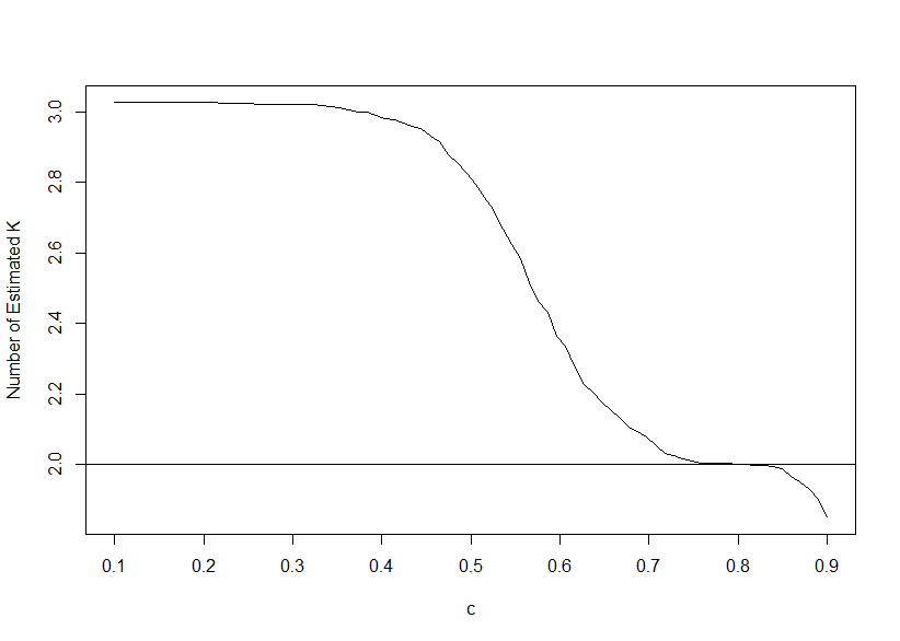
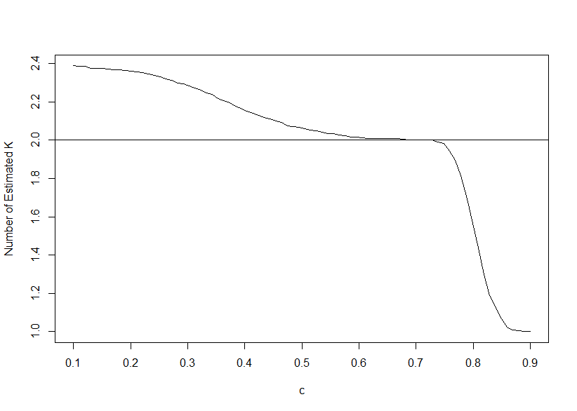
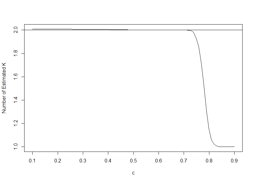
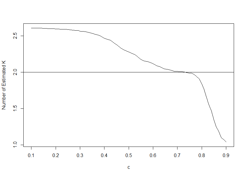
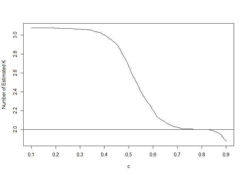
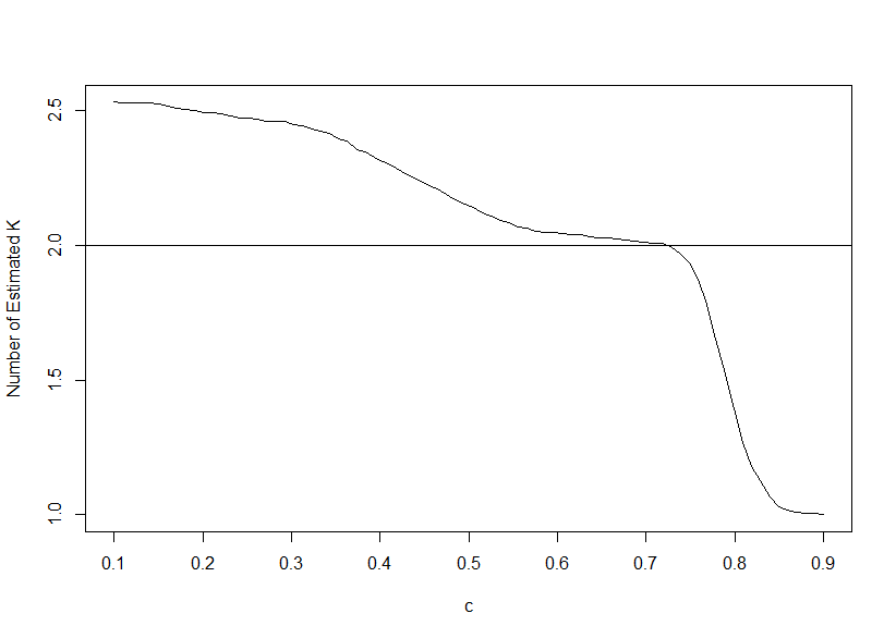
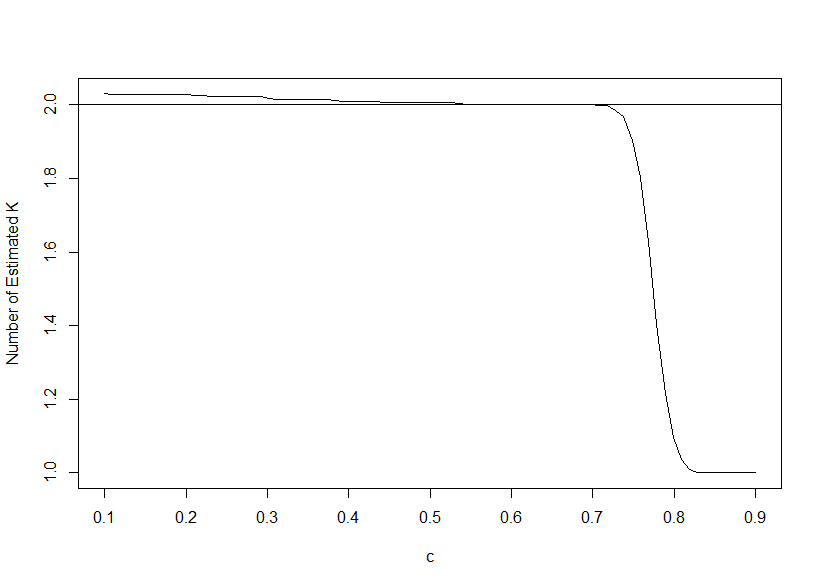
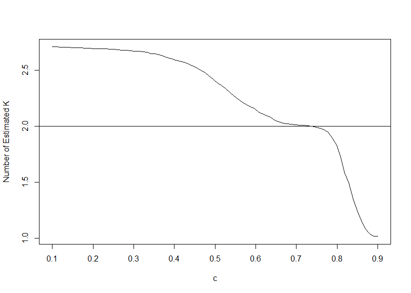
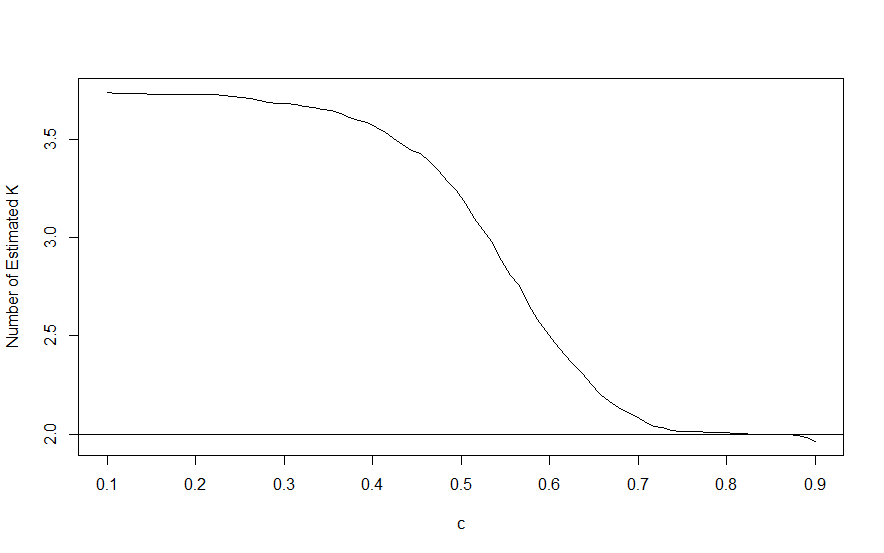
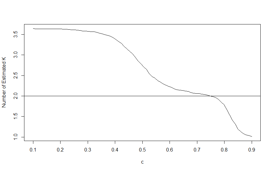
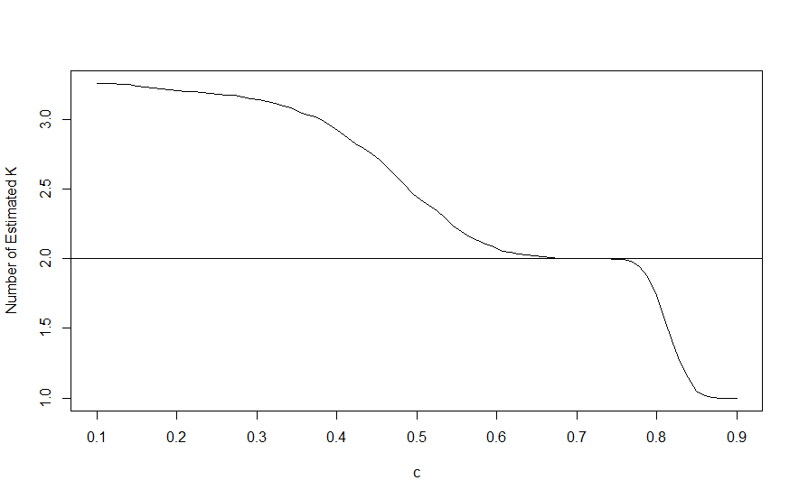
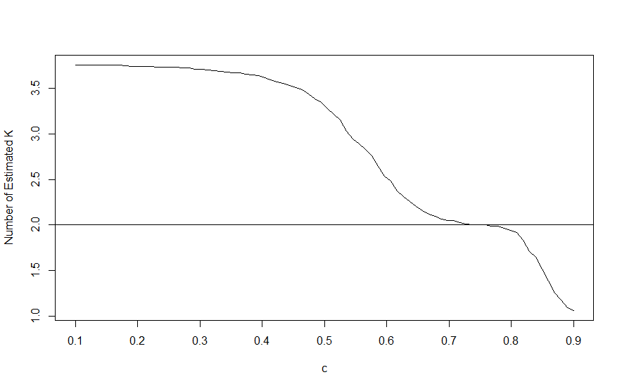
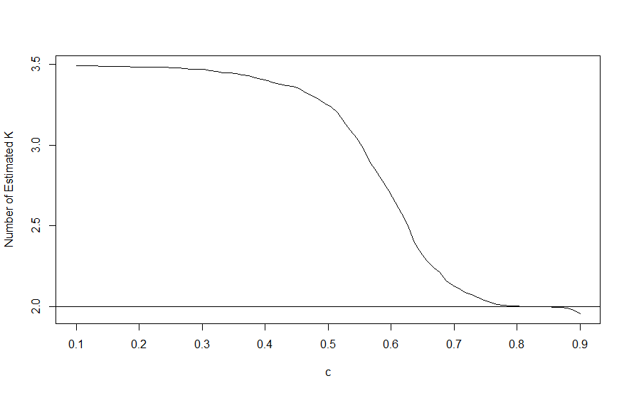
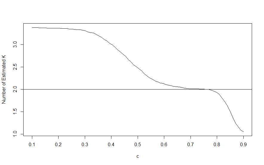
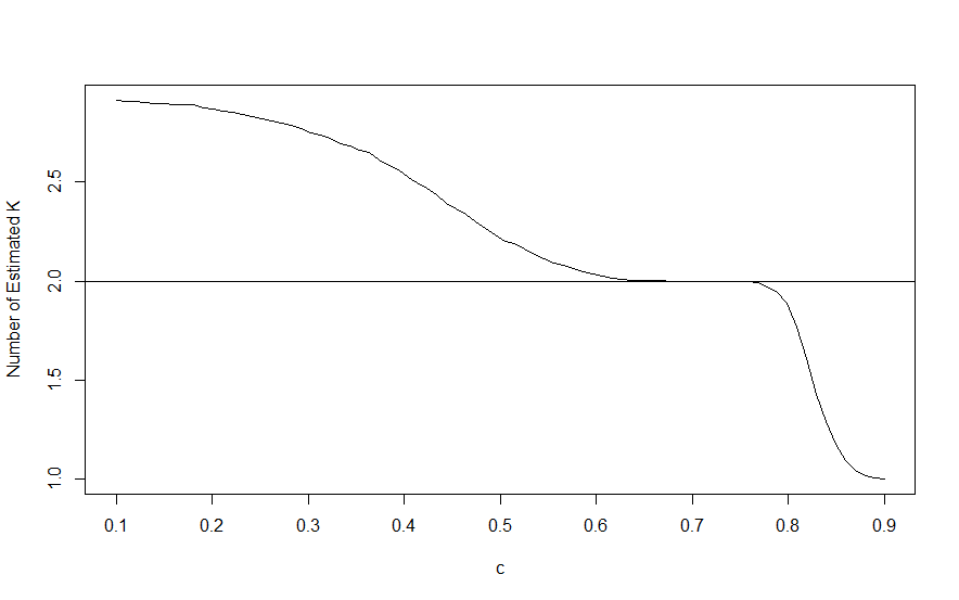
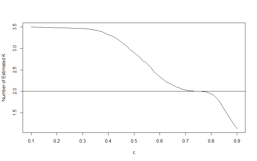
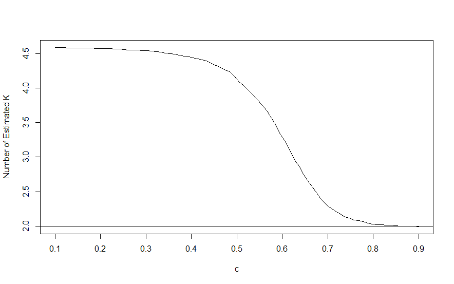
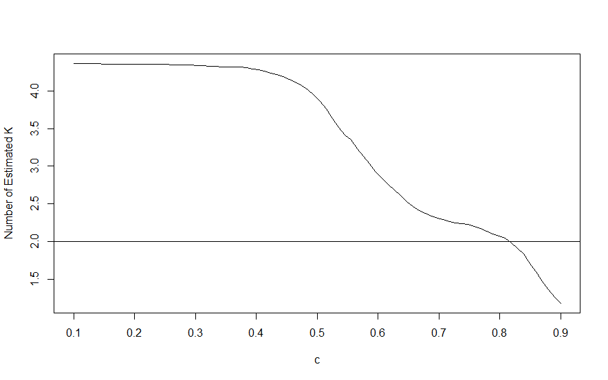
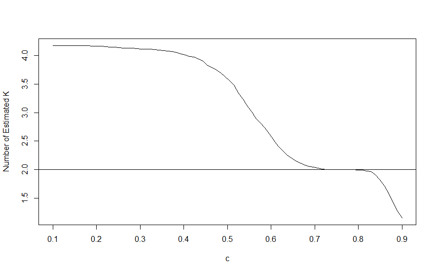
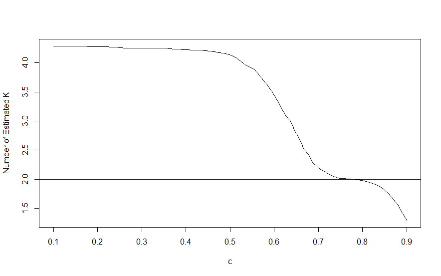
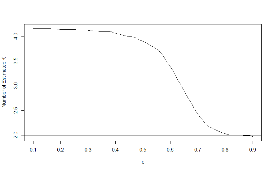
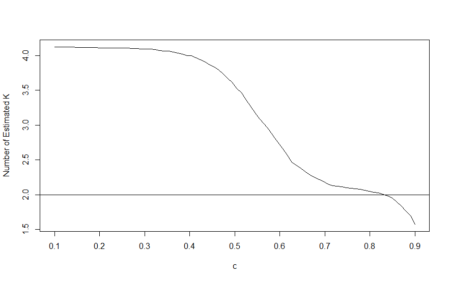
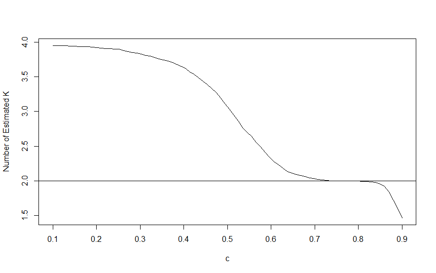
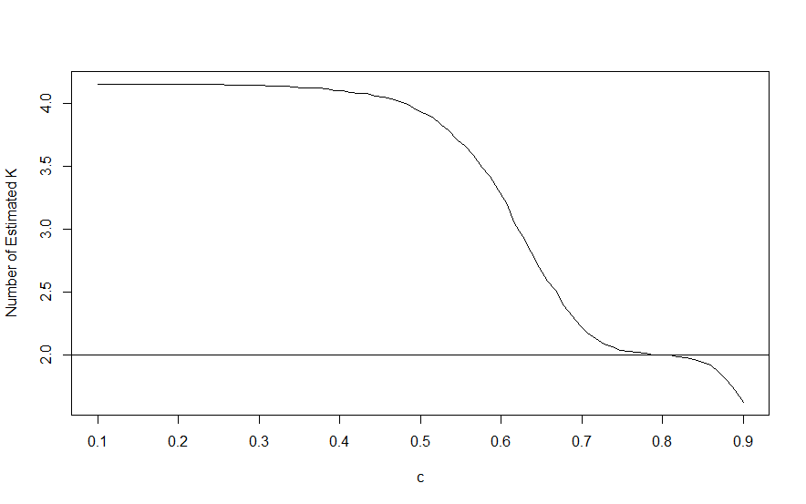
In BIC criterion, another problem is how to choose . Although we can set to satisfy conditions in Theorem 2, this choice may be too large which leads to underestimation of . To overcome this difficulty, we first choose a length, which equals , then compute the median, denoted by , for all values of the function below:
, .
is the estimated spectral density function from , is its integral. Finally, . Our simulation shows that an appropriate choice for is 0.73 regardless of .
The selection of spectral windows is an important topic in spectral estimation. In Priestley
(1981), bandwidth is selected as follows
,
where , where is the inverse Fourier transformation of , and is the largest integer so that the limit aforementioned exists and is non-zero. is the scale parameter in spectral windows. By the proofs of Theorem 1, we can see that estimators of change points reach consistency because dominate convergence rate. So bandwidth selection does not matter too much, which is verified by our simulations.
In application, sometimes sample size is large. Although we can apply some methods, such as screening, PELT, to boost the calculation, the computational complexity is still intolerable. Here, we set a change point searching unit, denoted by (Hawkins 2001). That is, when searching for change points, we add a unit of observations into our calculation each time, not just one observation. This unit is different from , which is used to calculate spectrums since estimating spectral density function usually needs sufficient amount of observations. By setting this unit, change point can only be estimated at , , , and so on. If we set this unit equal to 1, the algorithm degenerates to the general scenario when no searching unit is given. This will dramatically increase the speed of our algorithm. The computational complexity of Dynamic Programming is (Zou et al. 2014), so by setting a searching unit , the complexity will drop to . Apparently the estimation accuracy will be sacrificed, since the true change points and the maximizers of objective function, may not lie on the grid. We suggest the choice of by choosing the desired estimation accuracy first. Intuitively speaking, if we want the estimates having the accuracy of of the total sample size, then we can set .
Appendix A Proofs
In the appendix, to are appropriate constant and , are constant with respect to .
Lemma 1.
Suppose , , where . . Denote as the spectral density function of . is the estimated spectral density function. Then under Assumptions 1-6,
Proof: Following the method of Woodroofe and Van Ness (1967), we separate our proofs into 3 parts.
Part 1: we show that for given , . Here is the smoothed spectral density estimation for ,
|
|
|
|
|
|
|
|
|
|
|
|
|
|
|
|
|
|
|
|
where ,
,
,
.
Since for any real number , . So we only need to prove that , , are . By Markov’s inequality, it suffices to show that , , are .
After expanding , we have
|
|
|
|
|
|
|
|
|
|
where . If for any , then expectation of is not zero. If one of is 1, for example, , since for any , it is impossible to find in , so the expectation would be zero. To sum up, for all non-zero terms in , should be greater than 2. Since for any , , , can be bounded by a real number, denoted by , so we only need to count the number of non-zero terms. When for any , then , and the number of non-zero terms are no more than . When at least one of , say , the number of non-zero terms is no more than . So
.
For
,
we can see that for any in all non-zero terms, so following the discussions above, we have
.
By far, we have proven that and are .
|
|
|
|
|
|
|
|
|
|
|
|
|
|
|
First, when for any , , the number of terms after expanding is . So for fixed , contains no more than terms. What is more, for any fixed , the number for all possible , of which the power satisfy , is no more than . So there are no more than terms, which means that .
When and some of are equal to 1, we assume that . For , should satisfy , that is, . If not, since is independent of ,
, we have
.
So the number of all non-zero terms is no more than . For , there are terms which contain . So there are terms which do not contain . Then the number of non-zero terms is O(. For , if , contain , then it is easy to see that there are totally no more than terms which do not contain . However, now for all , . So the number of all possible non-zero terms is . Hence .
When , there are at least of , so following the discussions above, . Therefore summarizing discussions above, .
Part 2, we prove that .
|
|
|
|
|
|
|
|
|
|
And
|
|
|
|
|
|
|
|
|
|
|
|
|
|
|
Since , we have .
And
|
|
|
|
|
|
|
|
|
|
Since by Woodroofe and Van Ness (1967),
,
where is a constant. So
|
|
|
|
|
|
|
|
|
|
And . So we complete Part 2.
Part 3: we show that .
|
|
|
|
|
|
|
|
|
|
|
|
|
|
|
|
|
|
|
|
|
|
|
|
|
|
|
|
|
|
|
|
|
|
|
|
|
|
|
|
where is the periodogram for , is a constant. After some manipulations (see Woodroofe and Van Ness 1967, Grenander and Rosenblatt 1957).
|
|
|
|
|
|
|
|
|
|
|
|
|
|
|
|
|
|
|
|
Now let us focus on , that is , , and denote as the autocovariance function of .
|
|
|
|
|
|
|
|
|
|
|
|
|
|
|
|
|
|
|
|
|
|
|
|
|
|
|
|
|
|
|
|
|
|
|
Again, we only need to prove that the expectation of and are . And
|
|
|
|
|
|
|
|
|
|
|
|
|
|
|
|
|
|
|
|
|
|
|
|
|
|
|
|
|
|
|
|
|
|
|
For those four terms in the last inequality above, following the proofs in Part 1, we can show that each of them is . Similarly to the discussions above, . So we have . When some of are different from each other, for example, for , then in , the number of non-zero terms should be less than because some in are not in . And now, when the power of is 1 in the expansion of , we can not find any in , so the expectations of these terms are 0. So,
|
|
|
Since ,
for any given . Since , .
|
|
|
|
|
|
|
|
|
|
|
|
|
|
|
|
|
|
|
|
|
|
|
|
|
|
|
|
|
|
|
|
|
|
|
|
|
|
|
|
|
|
|
|
|
|
|
|
|
|
where the second inequality holds because of Hölder inequality, and is the Fourier transformation of the th derivative of . Since for , we have for , and
is bounded. So similar to Part 1, we have . Here we complete Part 3.
Since
|
|
|
|
|
|
|
|
|
|
|
|
|
|
|
we have
.
Then, by Markov inequality,
|
|
|
|
|
|
|
|
|
|
|
|
|
|
|
|
|
|
|
|
So
|
|
|
Here we complete the proof of Lemma 1.
Lemma 2.
Suppose , satisfy Assumptions 1-8, then
|
|
|
(1) |
|
|
|
(2) |
Proof:
|
|
|
|
|
|
|
|
|
|
|
|
|
|
|
|
|
|
|
|
|
|
|
|
|
|
|
|
|
|
|
|
|
|
|
where . So
|
|
|
|
|
|
|
|
|
|
|
|
|
|
|
|
|
|
|
|
By Lemma 1, we only need to show that
.
What is more, assume without loss of generality, then we have
|
|
|
|
|
|
|
|
|
|
|
|
|
|
|
|
|
|
|
|
|
|
|
|
|
|
|
|
|
|
Since , , for , so if , . So without loss of generality, we set , . Next, we separate the proofs into 2 parts, as in Lemma 1.
Part 1:
|
|
|
|
|
|
|
|
|
|
|
|
|
|
|
So
|
|
|
|
|
|
|
|
|
|
|
|
|
|
|
So for two terms in the inequality above, following the proofs in Part 1 of Lemma 1, we have
,
.
Part 2: Set , satisfying , , where denotes the conjugate of . We show that .
|
|
|
|
|
|
|
|
|
|
|
|
|
|
|
|
|
|
|
|
|
|
|
|
|
Since , all satisfy uniform Lipschitz condition, then it is easy to see that also satisfies uniform Lipschitz condition. Following the proofs in Part 3 of Lemma 1, we have
.
Following the proofs in Part 3 of Lemma 1 again, we have , where
|
|
|
|
|
|
|
|
|
|
So following the proofs in Part 3 of Lemma 1 again. we have
.
Here we complete the proof of Lemma 2.
Lemma 3.
Assume Assumption 1-8, , , when . Here
Proof: Set , and to are all constant. By Lemma 1, we have
,
So denote , then on set ,
, , .
Since ,
.
So on set , we have
|
|
|
|
|
|
|
|
|
|
|
|
|
|
|
Then on ,
|
|
|
|
|
|
|
|
|
|
|
|
|
|
|
|
|
|
|
|
|
|
|
|
|
|
|
|
|
|
|
|
|
|
|
Here is some constant containing . So set ,
|
|
|
|
|
|
|
|
|
|
|
|
|
|
|
|
|
|
|
|
and the last inequality can be arbitrarily small by choosing sufficiently large . Here we complete proofs of Lemma 3.
Lemma 4.
Assume Assumption 1-8, , , when . Here
Proof: Following the proofs of Lemma 3, this lemma can be easily obtained.
Proofs of Theorem 1:
Denote , where is the event in probability space . Then , we prove that , .
For , since is bounded, , then there exists such that on the subsequence. It follows from Lemma 2 and 3, that
,
where , . If , then by Lemma 3, we have
.
Since .
So
|
|
|
|
|
|
|
|
|
|
|
|
|
|
|
as , since every term above is always negative. If , then
|
|
|
So we have
|
|
|
as .
This is a contradiction because are the maximizers of . Since
.
so .
If , then there should be a change point that can not estimated consistently. Then following the proof in Theorem 1,
|
|
|
|
|
|
|
|
|
|
as .
If , then still every change point should be estimated consistently. So, there should be a change point . Then by Lemma 2 and 3, . So , as . Here we complete the proofs of Theorem 2.