Sharing Energy Storage Between
Transmission and Distribution

Abstract

This paper addresses the problem of how best to coordinate, or “stack,” energy storage services in systems that lack centralized markets. Specifically, its focus is on how to coordinate transmission-level congestion relief with local, distribution-level objectives. We describe and demonstrate a unified communication and optimization framework for performing this coordination. The congestion relief problem formulation employs a weighted ${\ell_{1}\text{-norm}}$ objective. This approach determines a set of corrective actions, i.e., energy storage injections and conventional generation adjustments, that minimize the required deviations from a planned schedule. To exercise this coordination framework, we present two case studies. The first is based on a 3-bus test system, and the second on a realistic representation of the Pacific Northwest region of the United States. The results indicate that the scheduling methodology provides congestion relief, cost savings, and improved renewable energy integration. The large-scale case study informed the design of a live demonstration carried out in partnership with the University of Washington, Doosan GridTech, Snohomish County PUD, and the Bonneville Power Administration. The goal of the demonstration was to test the feasibility of the scheduling framework in a production environment with real-world energy storage assets. The demonstration results were consistent with computational simulations.

I Introduction

Utility-scale energy storage has the potential to provide non-wire solutions to longstanding power grid problems. For example, distribution system operators (DSOs) could use energy storage to help reduce energy imbalance expenses or to serve their load more economically through energy arbitrage. Likewise, transmission system operators (TSOs) could use energy storage to mitigate congestion or provide frequency regulation. While the prospect of employing energy storage to tackle these challenges has drawn immense interest, the question of how best to coordinate, or “stack,” services remains open. A systematic approach to service coordination would not only help maximize resource utilization, but also bolster the financial viability of energy storage projects.

In this work, we describe and demonstrate a unified communication and optimization framework for scheduling multiple simultaneous storage services between a TSO and one or more DSOs. To address this problem, we propose a multistage approach based on mixed-integer linear programming. To demonstrate the viability of the framework, it was implemented and used to control a utility-scale battery energy storage system (ESS) in Everett, WA. This battery is owned and operated by Snohomish County PUD (SnoPUD), and offers services to the Bonneville Power Administration (BPA).

The scheduling framework presented here reflects the operating environment of the Pacific Northwest region of the United States; however, it is also suitable for systems that lack centralized markets or that rely heavily upon bilateral contracts. This is the case, for example, in large parts of Europe [1]. Furthermore, the ideas developed in this paper may inspire new approaches to energy storage scheduling in systems that do have centralized markets.

I-A Literature review

The concept of providing multiple simultaneous services with storage resources has generated active discussion throughout academia, industry, and government. The business case for multiple service provision in wholesale and retail markets is assessed by Teng and Strbac in [2]. Related economic analyses can be found in [3, 4, 5]. In contrast to [2], which focuses on the aggregation of distributed storage systems, we concentrate on independently scheduled utility-scale systems.

The problem of scheduling multiple services is addressed in [6, 7, 8, 9]. For previous work on sharing storage resources among multiple parties, see [10, 11, 12, 13]. In [6], Mégel et al. employ a model predictive control approach for co-optimizing simultaneous provision of local and system-wide services. The algorithm proposed therein determines the optimal power and energy capacity to allocate for each service as a function of time. Alternatively, we take a decentralized approach that permits the resource to determine the capacity required for local service provision. In regard to economics, [6] shows that stacking services can improve the financial prospects of storage resources.

Providing transmission-level congestion relief with energy storage is explored in [14, 15, 16, 17]. The related problem of employing energy storage in congestion-constrained distribution networks is considered in [18]. The multi-objective formulation developed by Khani et al. in [17] seeks to maximize ESS revenue generated via arbitrage and the ESS contribution to congestion relief. Balancing the two objectives is achieved using an adaptive penalty mechanism. This mechanism has a similar mathematical structure to the weighted ${\ell_{1}\text{-norm}}$ employed in the formulation we present in Section III.

Regulatory agencies and independent system operators have taken steps to facilitate the integration of storage resources into markets for electricity and ancillary services. In a notice of proposed rulemaking [19], FERC states that permitting storage resources to manage their own state of charge would “allow these resources to optimize their operations to provide all of the services that they are technically capable of providing.” We have adopted this perspective in the service coordination framework developed in this paper. In line with FERC’s guidance, CAISO has held workshops on the governance of storage resources for multiple-use applications [20].

I-B Paper organization

The remainder of this paper is organized as follows. Section II describes the method behind the linked communication and optimization procedures. It also outlines the reports that facilitate communication between parties. The formulation of the congestion relief optimization problem is presented in Section III. In Sections IV and V, we discuss results from the case studies and live demonstration. Section VII summarizes and concludes.

II Proposed method

TABLE I: Description of the reports

Name	Contents
Capacity	ESS power and energy capacity
Congestion forecast	Load forecast and TEPO charging indicator
Initial schedule	Initial DEPO injection schedule
Mitigation needs	Minimum and maximum net load
Final schedule	Final ESS combined injection schedule

The framework developed in this paper is an interlinked series of optimization problems and data transfers. We refer to the transmission grid energy positioning optimizer as TEPO and its counterpart in the distribution grid as DEPO. TEPO utilizes available energy storage capacity to satisfy transmission-side objectives, and DEPO seeks to satisfy local, distribution-side objectives.

The communication between TEPO and a given DEPO instance is based on five reports that are exchanged when their contents are required by a particular stage of the optimization. Table I outlines the contents of these reports, and Table II the sequence in which they are exchanged. This scheme complies with the OpenADR specification, an open and interoperable information exchange model for smart grid applications [21, 22]. In its simplest form, the procedure in Table II represents an exchange between two parties; however, there is no restriction on the number of DEPO instances with which TEPO may communicate. Each DEPO instance corresponds to a distribution-side entity or a subset of a given entity’s storage resources. In this way, the framework accommodates service coordination between a transmission system operator and an arbitrary number of additional parties.

TABLE II: Communication procedure

Direction	Capacity exchange
TEPO$\,\rightarrow\,$DEPO	TEPO requests the capacity report.
TEPO$\,\leftarrow\,$DEPO	DEPO returns the capacity report.
Direction	Congestion forecast exchange
TEPO$\,\rightarrow\,$DEPO	TEPO requests the initial schedule report.
TEPO$\,\leftarrow\,$DEPO	DEPO requests the congestion forecast report.
TEPO$\,\rightarrow\,$DEPO	TEPO returns the congestion forecast report.
TEPO$\,\leftarrow\,$DEPO	DEPO returns the initial schedule report.
Direction	Mitigation needs exchange
TEPO$\,\rightarrow\,$DEPO	TEPO requests the final schedule report.
TEPO$\,\leftarrow\,$DEPO	DEPO requests the mitigation needs report.
TEPO$\,\rightarrow\,$DEPO	TEPO returns the mitigation needs report.
TEPO$\,\leftarrow\,$DEPO	DEPO returns the final schedule report.

Here we explain the chain of data transfers for the basic case with one DEPO instance corresponding to a single ESS. Fig.​ 1 shows the interconnection of a typical ESS with the transmission grid. Fig.​ 2 shows the relationship between the communication procedure and the TEPO formulation. Initiating the procedure, TEPO requests the Capacity report from DEPO. This prompts DEPO to share information about the power rating and energy capacity of the ESS. Based on this information and the anticipated system operating conditions, TEPO provides DEPO with the Congestion forecast report. This report contains a forecast of the demand at the bus where the ESS is located and a charging indicator that flags whether TEPO would like to charge or discharge the ESS in each period of the optimization horizon. DEPO uses this information to generate a preliminary ESS schedule that it shares in the Initial schedule report. TEPO then processes DEPO’s initial schedule and generates its preferred supplemental injections. These are transmitted to DEPO in the form of bounds on the net load at the energy storage bus in the Mitigation needs report. After receiving the net load bounds, DEPO finalizes the ESS schedule and notifies TEPO through the Final schedule report. This concludes the procedure.

II-A Hour-ahead framework

The scheduling method presented here comprises both day-ahead and hour-ahead components. The purpose of the hour-ahead framework is to reassess the day-ahead schedule and account for changes in the system operating conditions, e.g., the load and renewable energy forecasts. This reassessment reflects the fact that there is less uncertainty in the hour-ahead framework than in the day-ahead. The flow of information is effectively the same as in Fig.​ 2, except the routine is solved iteratively over a shorter time horizon.

III Formulation

The exchange of information delineated in Table II is designed to support a multistage optimization framework. Here we envision a TEPO formulation that provides transmission-level congestion relief; however, other services, such as frequency regulation could also be handled under this framework. DEPO has the flexibility to run a separate optimization or control scheme that oversees local service provision. Table III outlines a set nomenclature for the TEPO formulation, and Table IV the optimization stages. The relationship between the TEPO formulation and the communication procedure is shown in Fig.​ 2. At a high level, each stage of the formulation can be stated as

$$\begin{array}[]{l l l}\displaystyle{\mathop{\mathrm{minimize}}_{\xi}}&f(\xi),\\ \mathrm{subject\ to}&\mkern 2.0mug_{r}(\xi)\leq 0,&r\in\mathopen{}\mathclose{{}\left\{1,\dots,p}\right\},\\ &h_{r}(\xi)=0,&r\in\mathopen{}\mathclose{{}\left\{1,\dots,q}\right\},\end{array}$$ (1)

where $\xi$ denotes an ordered list, or tuple, of decision variables. The inequality constraints are denoted by ${\{g_{r}\}_{r=1}^{p}}$, and the equality constraints by ${\{h_{r}\}_{r=1}^{q}}$.

III-A Stage $1$, Pre-mitigation unit commitment

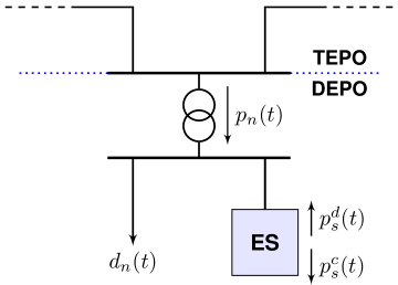
Figure 1: Representative interconnection diagram for an ESS.

TABLE III: Set nomenclature

Set	Index	Description
$\mathcal{B}$	$b$	Generator cost curve segments
$\mathcal{I}$	$i$	Conventional generators
$\mathcal{J}$	$j$	Fixed generators
$\mathcal{K}$	$k$	Solar power plants
$\mathcal{L}$	$l$	Transmission lines
$\mathcal{N}$	$n$	Buses
$\mathcal{S}$	$s$	Storage devices
$\mathcal{T}$	$t$	Time intervals
$\mathcal{W}$	$w$	Wind farms

Stage $1$ is called the Pre-mitigation unit commitment problem. In it, TEPO solves a standard unit commitment and economic dispatch without taking energy storage or system security constraints into account. The output corresponds to the optimal commitment and dispatch irrespective of energy storage and transmission capacity.

III-A1 Decision variables

The tuple of decision variables in Stage $1$ is

$$\xi:\mathopen{}\mathclose{{}\left(v_{i},y_{i},z_{i},p_{ib},p_{i},x_{k},x_{w},\theta_{n}}\right),$$

for all ${b\in\mathcal{B}}$, ${i\in\mathcal{I}}$, ${k\in\mathcal{K}}$, ${n\in\mathcal{N}}$, ${w\in\mathcal{W}}$, and ${t\in\mathcal{T}}$, where the relevant sets are defined in Table III. For the $i$th conventional generation unit, $v_{i}$, $y_{i}$, and $z_{i}$ are the commitment, startup, and shutdown status variables, respectively. Correspondingly, $p_{i}$ is the total power output, and $p_{ib}$ is the power of the $b$th segment, or block, of its cost curve. For renewable generation, $x_{k}$ is the power curtailment of the $k$th solar plant, and $x_{w}$ the curtailment of the $w$th wind farm. Lastly, $\theta_{n}$ denotes the voltage angle at bus $n$.

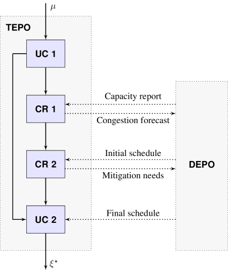
Figure 2: Day-ahead communication and optimization flow.

TABLE IV: Optimization stages

No.	Stage	Description
1	UC 1	Pre-mitigation stage
2	CR 1	Independent congestion relief
3	CR 2	Coordinated congestion relief
4	UC 2	Post-mitigation stage

III-A2 Objective function

For Stage $1$, we employ a standard minimum operating cost objective that can be separated into three components:

$$f(\xi)=\sum_{t\in\mathcal{T}}\sum_{i\in\mathcal{I}}C_{i}(t)+\sum_{t\in\mathcal{T}}\sum_{w\in\mathcal{W}}C_{w}(t)+\sum_{t\in\mathcal{T}}\sum_{k\in\mathcal{K}}C_{k}(t),$$ (2)

where $C_{i}$ is the total cost incurred by the $i$th conventional generating unit, while $C_{w}$ and $C_{k}$ account for the cost of curtailing wind and solar generation, respectively.

The conventional generation costs are given by

$$C_{i}(t)=c_{i}^{\mathrm{nl}}v_{i}(t)+c_{i}^{\mathrm{su}}y_{i}(t)+\sum_{b\in\mathcal{B}}m_{ib}\mkern 1.0mup_{ib}(t),$$ (3)

where $m_{ib}$ is the incremental cost of the $b$th block of unit $i$’s cost curve, $c_{i}^{\mathrm{nl}}$ is the no-load cost, and $c_{i}^{\mathrm{su}}$ the startup cost.

The costs arising from curtailing renewable generation are

$$C_{w}(t) =m_{w}x_{w}(t)$$ (4)

$$C_{k}(t) =m_{k}x_{k}(t),$$ (5)

where $m_{w}$ and $m_{k}$ denote the incremental costs of curtailing the $w$th wind farm and $k$th solar plant, respectively.

III-A3 Binary variable generation constraints

The startup and shutdown of unit $i$ is captured by the constraints

$$y_{i}(t)-z_{i}(t)=v_{i}(t)-v_{i}(t-1)$$ (6)

$$y_{i}(t)+z_{i}(t)\leq 1,$$ (7)

which are enforced for all ${i\in\mathcal{I}}$ and ${t\in\mathcal{T}}$. In the initial time period, ${v_{i}(t-1)}$ takes a special value, $v_{i}^{0}$, that reflects the initial commitment status of unit $i$.

III-A4 Minimum up and down time constraints

Let $\vphantom{L}\smash{\overline{L}}_{i}$ denote the number of time periods that unit $i$ must remain up at the beginning of the operating horizon, and let $\vphantom{L}\smash{\underline{L}}_{i}$ be the corresponding number of periods that it must remain down. These parameters are defined in [23]. At least one of $\vphantom{L}\smash{\overline{L}}_{i}$ and $\vphantom{L}\smash{\underline{L}}_{i}$ is zero by definition. To ensure that the commitment status of unit $i$ remains unchanged for the initial number of periods dictated by $\vphantom{L}\smash{\overline{L}}_{i}$ or $\vphantom{L}\smash{\underline{L}}_{i}$, the constraint

$$v_{i}(t)=v_{i}^{0},\text{ for all }t\leq\vphantom{L}\smash{\overline{L}}_{i}+\vphantom{L}\smash{\underline{L}}_{i},\\$$ (8)

is enforced for all ${i\in\mathcal{I}}$. The minimum up and down time requirements over the remainder of the operating horizon are given by

$$\sum_{\tau=t-\vphantom{\Gamma}\smash{\overline{\Gamma}}_{i}+1}^{t} y_{i}(\tau)\leq v_{i}(t),\text{ for all }t\geq\vphantom{L}\smash{\overline{L}}_{i}$$ (9)

$$\sum_{\tau=t-\vphantom{\Gamma}\smash{\underline{\Gamma}}_{i}+1}^{t} z_{i}(\tau)\leq 1-v_{i}(t),\text{ for all }t\geq\vphantom{L}\smash{\underline{L}}_{i},$$ (10)

for all ${i\in\mathcal{I}}$, where $\vphantom{\Gamma}\smash{\overline{\Gamma}}_{i}$ is the minimum up time, and $\vphantom{\Gamma}\smash{\underline{\Gamma}}_{i}$ the minimum down time.

III-A5 Generator output constraints

The total power output of the $i$th unit is given by sum of the outputs corresponding to the segments, or blocks, of its cost curve, i.e.,

$$p_{i}(t)=\sum_{b\in\mathcal{B}}p_{ib}(t),$$ (11)

for all ${i\in\mathcal{I}}$ and ${t\in\mathcal{T}}$. The conventional generator cost curves employed in Eq. 3 are piecewise-linear with segments ${b\in\mathcal{B}}$. Typically, the associated marginal cost curves are monotonically nondecreasing.

The power output of each block and the total output of each unit is bounded such that

$$\vphantom{p}\smash{\underline{p}}_{i}v_{i}(t) \leq p_{i}(t)\leq\vphantom{p}\smash{\overline{p}}_{i}v_{i}(t)$$ (12)

$$0 \leq p_{ib}(t)\leq\vphantom{p}\smash{\overline{p}}_{ib}v_{i}(t),$$ (13)

for all ${b\in\mathcal{B}}$, ${i\in\mathcal{I}}$, and ${t\in\mathcal{T}}$. For the $i$th unit, $\vphantom{p}\smash{\underline{p}}_{i}$ is the minimum power output, and $\vphantom{p}\smash{\overline{p}}_{i}$ the maximum power output. Similarly, $\vphantom{p}\smash{\overline{p}}_{ib}$ is the maximum output of the $b$th block of unit $i$’s cost curve. The maximum unit output, $\vphantom{p}\smash{\overline{p}}_{i}$, is permitted to vary between operating horizons to account for scheduled maintenance and forced outages.

III-A6 Ramping constraints

The ramping constraints on conventional generation are expressed as follows:

$$-\vphantom{R}\smash{\underline{R}}_{i}\leq p_{i}(t)-p_{i}(t-1)\leq\vphantom{R}\smash{\overline{R}}_{i},$$ (14)

for all ${i\in\mathcal{I}}$ and ${t\in\mathcal{T}}$, where $\vphantom{R}\smash{\overline{R}}_{i}$ is the upward ramp limit, and $\vphantom{R}\smash{\underline{R}}_{i}$ the downward ramp limit. In the initial time period, $p_{i}(t-1)$ takes a special value, $p_{i}^{0}$, that reflects the initial power output of the $i$th unit.

III-A7 Renewable generation curtailment constraints

Recall that the objective function stated in Eq. 2 includes terms that account for the cost of curtailing variable renewable generation. In accordance with Eq. 4 and Eq. 5, the constraints on curtailment are given by

$$0 \leq x_{w}(t)\leq p_{w}(t)$$ (15)

$$0 \leq x_{k}(t)\leq p_{k}(t),$$ (16)

where $p_{w}$ is the power available at the $w$th wind farm, and $p_{k}$ the power available at the $k$th solar plant. These constraints are enforced for all ${w\in\mathcal{W}}$, ${k\in\mathcal{K}}$, and ${t\in\mathcal{T}}$.

III-A8 Nodal power balance constraints

Power transfer throughout the transmission network is modeled using a standard dc power flow approximation, i.e.,

$$F_{l}(t)=\mathopen{}\mathclose{{}\left[\theta_{o(l)}\mkern 0.0mu(t)-\theta_{d(l)}\mkern 0.0mu(t)}\right]/x_{l},$$ (17)

for all ${l\in\mathcal{L}}$ and ${t\in\mathcal{T}}$. This network model encompasses high-voltage transmission lines for which the resistance to reactance ratio, $r_{l}/x_{l}$, may be reasonably assumed to be small [24, 25, 26]. For line $l$, $x_{l}$ is the reactance, and $F_{l}$ the real power flow. The function $o(l)$ returns the origin or “from” bus index of line $l$, and $d(l)$ returns the destination or “to” bus index. The voltage angles are bounded between $-\pi$ and $\pi$ for all ${n\in\mathcal{N}}$ and ${t\in\mathcal{T}}$. Per convention, the reference bus is constrained to have a voltage angle of zero for all ${t\in\mathcal{T}}$.

Using Eq. 17, the nodal power balance constraints can be stated as follows:

$$d_{n}(t)=\sum_{i\in\mathcal{I}_{n}}p_{i}(t)+\sum_{j\in\mathcal{J}_{n}}p_{j}(t)+\sum_{k\in\mathcal{K}_{n}}\hat{p}_{k}(t)\\ +\sum_{w\in\mathcal{W}_{n}}\hat{p}_{w}(t)-\sum_{l\in\mathcal{O}_{n}}F_{l}(t)+\sum_{l\in\mathcal{D}_{n}}F_{l}(t),$$ (18)

for all ${n\in\mathcal{N}}$ and ${t\in\mathcal{T}}$, where $d_{n}$ is the total demand at bus $n$. Let a subscript $n$ affixed to a set indicate the subset of components connected to bus $n$. The set of lines originating at bus $n$ is denoted by $\mathcal{O}_{n}$, and the set with destinations at bus $n$ by $\mathcal{D}_{n}$. The net power from the $k$th solar plant is ${\hat{p}_{k}(t)=p_{k}(t)-x_{k}(t)}$, and the net power from the $w$th wind farm ${\hat{p}_{w}(t)=p_{w}(t)-x_{w}(t)}$.

III-B Stage $2$, Independent congestion relief

Stage $2$ is called the Independent congestion relief problem because TEPO solves it without knowledge of the ESS schedule (or hour-ahead adjustments) that DEPO would like to carry out. Using the capacity report, TEPO solves an optimization to determine a minimal set of corrective actions, i.e., commitment and dispatch adjustments and ESS injections, required to alleviate congestion. This allows TEPO to form a cursory schedule indicating whether each ESS should be charged or discharged as a function of time to mitigate congestion.

At a high level, the objective of the congestion relief problem takes the form

$$f(\xi)=\sum_{r\in\mathcal{R}}\lvert\alpha_{r}\xi_{r}\rvert={\mathopen{}\mathclose{{}\left\lVert A\xi}\right\rVert}_{1},$$ (19)

where ${\alpha_{r}\geq 0}$ for all ${r\in\mathcal{R}}$. Let ${A\in\mathbb{R}^{\lvert\mathcal{R}\rvert\times\lvert\mathcal{R}\rvert}}$ be a real, positive-semidefinite diagonal matrix. Mathematically, Eq. 19 is a weighted ${\ell_{1}\text{-norm}}$ where $\alpha_{r}$ is the weight for the $r$th entry of $\xi$. Recall that the cardinality of $\xi$ is the number of nonzero entries it contains. Although cardinality minimization is NP-hard in general, for bounded systems of linear equalities and inequalities it is equivalent to ${\ell_{p}\text{-norm}}$ minimization [27]. As shown in [28], the ${\ell_{1}\text{-norm}}$ is the convex envelope, i.e., the best convex lower bound, of the cardinality function. For this reason, the ${\ell_{1}\text{-norm}}$ is used as a convex approximation to the cardinality function in statistical regression, compressed sensing, and elsewhere [29, 30]. Hence, the objective stated in (19) has the effect of minimizing the number of corrective actions required to alleviate congestion.

It is possible to formulate optimization problems with ${\ell_{1}\text{-norm}}$ objectives as linear programs, as described in [31]. Absolute value terms, such as ${\mathopen{}\mathclose{{}\left\lvert\alpha_{r}\xi_{r}}\right\rvert}$, can be implemented with auxiliary variables and constraints of the form

$$\xi_{r} ={\xi}^{{}\scriptscriptstyle{+}}_{r}-{\xi}^{{}\scriptscriptstyle{-}}_{r}$$ (20)

$$0 \leq{\xi}^{{}\scriptscriptstyle{+}}_{r},\ \ 0\leq{\xi}^{{}\scriptscriptstyle{-}}_{r}.$$ (21)

The absolute value is then given by

$$\mathopen{}\mathclose{{}\left\lvert\alpha_{r}\xi_{r}}\right\rvert=\lvert\alpha_{r}\rvert\mathopen{}\mathclose{{}\left({\xi}^{{}\scriptscriptstyle{+}}_{r}+{\xi}^{{}\scriptscriptstyle{-}}_{r}}\right),$$ (22)

or simply ${\alpha_{r}({\xi}^{{}\scriptscriptstyle{+}}_{r}+{\xi}^{{}\scriptscriptstyle{-}}_{r})}$ where ${\alpha_{r}\geq 0}$. Where necessary, binary variable constraints can be introduced to ensure that at most one of ${\xi}^{{}\scriptscriptstyle{+}}_{r}$ and ${\xi}^{{}\scriptscriptstyle{-}}_{r}$ is nonzero.

III-B1 Decision variables

The tuple of decision variables in Stage $2$ is

$$\xi:\bigl{(}v_{i},y_{i},z_{i},\nu_{s},\psi_{s},\zeta_{s},E_{s},\delta p_{ib},\delta p_{i},\delta p_{s}^{c},\delta p_{s}^{d},\delta x_{w},\delta x_{k}\bigr{)},$$

for all ${b\in\mathcal{B}}$, ${i\in\mathcal{I}}$, ${k\in\mathcal{K}}$, ${n\in\mathcal{N}}$, ${s\in\mathcal{S}}$, ${w\in\mathcal{W}}$, and ${t\in\mathcal{T}}$. The conventional generation binary variables are defined as in Stage $1$. The energy storage binary variables $\nu_{s}$, $\psi_{s}$, and $\zeta_{s}$ prevent simultaneous charging and discharging (and simultaneous opposing adjustments). The state of charge (SOC) of the $s$th ESS is denoted by $E_{s}$. Let variables beginning with $\delta$ denote adjustments or deviations in some underlying quantity. For example, $\delta p_{s}^{c}$ is the charging adjustment of the $s$th ESS, and $\delta p_{s}^{d}$ the corresponding discharging adjustment. Each of these deviations is implemented with a pair of nonnegative decision variables as in Eq. 20–Eq. 22.

III-B2 Objective function

In this case, the objective function does not correspond precisely to an economic cost. Rather, it represents a penalty for deviating from the schedule determined in Stage $1$. For Stage $2$, the objective function can be separated into four components:

$$f(\xi)=\sum_{t\in\mathcal{T}}\sum_{i\in\mathcal{I}}\Phi_{i}(t)+\sum_{t\in\mathcal{T}}\sum_{w\in\mathcal{W}}\Phi_{w}(t)\\ +\sum_{t\in\mathcal{T}}\sum_{k\in\mathcal{K}}\Phi_{k}(t)+\sum_{t\in\mathcal{T}}\sum_{s\in\mathcal{S}}\Phi_{s}(t),$$ (23)

where $\Phi_{i}$, $\Phi_{w}$, $\Phi_{k}$, and $\Phi_{s}$ are penalty functions.

The conventional generation adjustment penalty function is

$$\Phi_{i}(t)=c_{i}^{\mathrm{nl}}v_{i}(t)+c_{i}^{\mathrm{su}}y_{i}(t)\\ +\sum_{b\in\mathcal{B}}\rho_{ib}\mathopen{}\mathclose{{}\left[\delta{p}^{{}\scriptscriptstyle{+}}_{ib}(t)+\delta{p}^{{}\scriptscriptstyle{-}}_{ib}(t)}\right],$$ (24)

where $\rho_{ib}$ is an incremental penalty on adjusting generation dispatch. The no-load and startup costs are included to ensure changes in commitment are reflected in the objective.

The penalties arising from renewable generation curtailment adjustments are given by

$$\Phi_{w}(t) =\rho_{w}\mathopen{}\mathclose{{}\left[\delta{x}^{{}\scriptscriptstyle{+}}_{w}(t)+\delta{x}^{{}\scriptscriptstyle{-}}_{w}(t)}\right]$$ (25)

$$\Phi_{k}(t) =\rho_{k}\mathopen{}\mathclose{{}\left[\delta{x}^{{}\scriptscriptstyle{+}}_{k}(t)+\delta{x}^{{}\scriptscriptstyle{-}}_{k}(t)}\right],$$ (26)

where $\rho_{w}$ and $\rho_{k}$ are incremental penalties on adjusting wind and solar curtailment, respectively.

Lastly, the penalty associated with energy storage charging and discharging is given by

$$\Phi_{s}(t)=\rho_{s}\mathopen{}\mathclose{{}\left[\delta{p}_{s}^{c}(t)+\delta{p}_{s}^{d}(t)}\right],$$ (27)

where $\rho_{s}$ is an incremental penalty on adjusting ESS injections. This function is equivalent to penalizing the total charging and discharging amounts because it differs only by a constant. For the complete energy storage model, refer to Section III-B7.

III-B3 Generator output adjustment constraints

The binary variable generation constraints and minimum up and down time constraints in Stage $2$ are identical to those in Stage $1$; however, the generator output constraints require modification. Let $p_{ib}$ and $p_{i}$ be the block and unit outputs determined in Stage $1$. Conventional generation output is then bounded by

$$\vphantom{p}\smash{\underline{p}}_{i}v_{i}(t)\leq p_{i}(t) +\delta{p}^{{}\scriptscriptstyle{+}}_{i}(t)-\delta{p}^{{}\scriptscriptstyle{-}}_{i}(t)\leq\vphantom{p}\smash{\overline{p}}_{i}v_{i}(t)$$ (28)

$$0\leq p_{ib}(t) +\delta{p}^{{}\scriptscriptstyle{+}}_{ib}(t)-\delta{p}^{{}\scriptscriptstyle{-}}_{ib}(t)\leq\vphantom{p}\smash{\overline{p}}_{ib}v_{i}(t),$$ (29)

for all ${b\in\mathcal{B}}$, ${i\in\mathcal{I}}$, and ${t\in\mathcal{T}}$. As in Eq. 11, unit and block output are related by

$$p_{i}(t)+\delta{p}^{{}\scriptscriptstyle{+}}_{i}(t)-\delta{p}^{{}\scriptscriptstyle{-}}_{i}(t)=\\ \sum_{b\in\mathcal{B}}\mathopen{}\mathclose{{}\left[p_{ib}(t)+\delta{p}^{{}\scriptscriptstyle{+}}_{ib}(t)-\delta{p}^{{}\scriptscriptstyle{-}}_{ib}(t)}\right],$$ (30)

for all ${i\in\mathcal{I}}$ and ${t\in\mathcal{T}}$.

III-B4 Ramping constraints

In Stage $2$, conventional generation ramp rates are limited such that

$$-\vphantom{R}\smash{\underline{R}}_{i} \leq p_{i}(t)+\delta{p}^{{}\scriptscriptstyle{+}}_{i}(t)-\delta{p}^{{}\scriptscriptstyle{-}}_{i}(t)$$

$$\quad-p_{i}(t-1)-\delta{p}^{{}\scriptscriptstyle{+}}_{i}(t-1)+\delta{p}^{{}\scriptscriptstyle{-}}_{i}(t-1)\leq\vphantom{R}\smash{\overline{R}}_{i},$$ (31)

for all ${i\in\mathcal{I}}$ and ${t\in\mathcal{T}}$. This constraint follows from Eq. 14.

III-B5 Nodal power balance and transmission constraints

The nodal power balance constraints have the same structure as Eq. 18, with the exception that the power terms are augmented to account for curtailments and dispatch adjustments. Since the objective of Stage $2$ is to determine a minimal set of corrective actions required to alleviate congestion, we introduce transmission constraints of the form

$$\vphantom{F}\smash{\underline{F}}_{l}\leq F_{l}(t)\leq\vphantom{F}\smash{\overline{F}}_{l}\text{ for all }l\in\mathcal{L}_{m}\text{ and }t\in\mathcal{T},$$ (32)

where $\mathcal{L}_{m}$ denotes the set of monitored lines such that ${\mathcal{L}_{m}\subseteq\mathcal{L}}$. For symmetric bidirectional flow limits, we have ${\vphantom{F}\smash{\underline{F}}_{l}=-\vphantom{F}\smash{\overline{F}}_{l}}$.

III-B6 Renewable generation curtailment adjustment constraints

As in Eq. 15 and Eq. 16, curtailment levels are bounded such that

$$0 \leq x_{w}(t)+\delta{x}^{{}\scriptscriptstyle{+}}_{w}(t)-\delta{x}^{{}\scriptscriptstyle{-}}_{w}(t)\leq p_{w}(t)$$ (33)

$$0 \leq x_{k}(t)+\delta{x}^{{}\scriptscriptstyle{+}}_{k}(t)-\delta{x}^{{}\scriptscriptstyle{-}}_{k}(t)\leq p_{k}(t),$$ (34)

for all ${w\in\mathcal{W}}$, ${k\in\mathcal{K}}$, and ${t\in\mathcal{T}}$.

III-B7 Energy storage constraints

The total energy storage charging and discharging amounts are given by

$$p_{s}^{c}(t) =p_{s}^{c_{0}}\mkern 0.0mu(t)+\delta{p}^{{c}\scriptscriptstyle{+}}_{s}\mkern 0.0mu(t)-\delta{p}^{{c}\scriptscriptstyle{-}}_{s}\mkern 0.0mu(t)$$ (35)

$$p_{s}^{d}(t) =p_{s}^{d_{0}}\mkern 0.0mu(t)+\delta{p}^{{d}\scriptscriptstyle{+}}_{s}\mkern 0.0mu(t)-\delta{p}^{{d}\scriptscriptstyle{-}}_{s}\mkern 0.0mu(t),$$ (36)

where $p_{s}^{c_{0}}$ is the initial charging schedule, and $p_{s}^{d_{0}}$ the initial discharging schedule. In Stage $2$ of the day-ahead formulation ${p_{s}^{c_{0}}(t)=p_{s}^{d_{0}}(t)=0}$ for all ${t\in\mathcal{T}}$ because neither party has proposed a nonzero ESS injection schedule. For a complete breakdown of these initial conditions by stage, refer to Table V and Section III-B8.

The charging and discharging decision variables are nonnegative and bounded above such that

$$0 \leq p_{s}^{c}(t)\leq\vphantom{p}\smash{\overline{p}}_{s}^{c}\nu_{s}(t)$$ (37)

$$0 \leq p_{s}^{d}(t)\leq\vphantom{p}\smash{\overline{p}}_{s}^{d}[1-\nu_{s}(t)],$$ (38)

where $\vphantom{p}\smash{\overline{p}}_{s}^{c}$ is the maximum charging power of the $s$th ESS, and $\vphantom{p}\smash{\overline{p}}_{s}^{d}$ the maximum discharging power. If the $s$th ESS is charging at time $t$, ${\nu_{s}(t)=1}$; otherwise, ${\nu_{s}(t)=0}$. Constraints Eq. 37 and Eq. 38 prohibit simultaneous charging and discharging. Similarly, the charging adjustments are nonnegative and bounded above such that

$$0 \leq\delta{p}^{{c}\scriptscriptstyle{+}}_{s}\mkern 0.0mu(t)\leq[\vphantom{p}\smash{\overline{p}}_{s}^{c}-p_{s}^{c_{0}}\mkern 0.0mu(t)]\psi_{s}(t)$$ (39)

$$0 \leq\delta{p}^{{c}\scriptscriptstyle{-}}_{s}\mkern 0.0mu(t)\leq p_{s}^{c_{0}}\mkern 0.0mu(t)[1-\psi_{s}(t)],$$ (40)

where ${\psi_{s}(t)=1}$ when the charging adjustment of the $s$th ESS is positive, and ${\psi_{s}(t)=0}$ otherwise. For the discharging adjustments, we have

$$0 \leq\delta{p}^{{d}\scriptscriptstyle{+}}_{s}\mkern 0.0mu(t)\leq[\vphantom{p}\smash{\overline{p}}_{s}^{d}-p_{s}^{d_{0}}\mkern 0.0mu(t)]\zeta_{s}(t)$$ (41)

$$0 \leq\delta{p}^{{d}\scriptscriptstyle{-}}_{s}\mkern 0.0mu(t)\leq p_{s}^{d_{0}}\mkern 0.0mu(t)[1-\zeta_{s}(t)],$$ (42)

where ${\zeta_{s}(t)=1}$ when the discharging adjustment of the $s$th ESS is positive, and ${\zeta_{s}(t)=0}$ otherwise. Constraints Eq. 35–Eq. 42 are enforced for all ${s\in\mathcal{S}}$ and ${t\in\mathcal{T}}$.

The formulation also includes a set of constraints that enable TEPO to respect ESS state of charge limitations. The difference equation that describes the SOC trajectory is given by

$$E_{s}(t) =E_{s}(t-1)+(\Delta\eta_{s}^{c})p_{s}^{c}(t)-(\Delta/\eta_{s}^{d})p_{s}^{d}(t),$$ (43)

for all ${s\in\mathcal{S}}$ and ${t\in\mathcal{T}}$, where $\Delta$ is the step size parameter. The charging efficiency of the $s$th ESS is denoted by $\eta_{s}^{c}$, and the discharging efficiency by $\eta_{s}^{d}$. The SOC is then bounded as follows:

$$\vphantom{E}\smash{\underline{E}}_{s}(t) \leq E_{s}(t)\leq\vphantom{E}\smash{\overline{E}}_{s}(t),$$ (44)

for all ${s\in\mathcal{S}}$ and ${t\in\mathcal{T}}$, where $\vphantom{E}\smash{\underline{E}}_{s}$ is the minimum SOC, and $\vphantom{E}\smash{\overline{E}}_{s}$ the maximum SOC. Additionally, we impose an equality constraint at the end of each day such that

$$E_{s}(t_{\mkern 0.0muf}) =E_{s}^{\prime},$$ (45)

for all ${s\in\mathcal{S}}$. The final time index of the day is $t_{\mkern 0.0muf}$, and the target SOC at ${t=t_{\mkern 0.0muf}}$ is $E_{s}^{\prime}$. This approach brings each ESS to a predictable SOC at the end of each day.

III-B8 Energy storage scheduling initial conditions by stage

The initial ESS charging and discharging schedules, denoted respectively by $p_{s}^{c_{0}}$ and $p_{s}^{d_{0}}$, vary with the optimization stage. In Stage $2$ of the day-ahead formulation, the initial schedules are zero-valued because neither party has proposed a set of injections. The schedules agreed upon at the conclusion of the day-ahead framework, denoted by $\tilde{p}_{s}^{c}$ and $\tilde{p}_{s}^{d}$, serve as the initial schedules for Stage $2$ of the hour-ahead framework. The schedule adjustments proposed by DEPO prior to Stage $3$ are denoted by $\delta\tilde{p}_{s}^{c}$ and $\delta\tilde{p}_{s}^{d}$. Table V provides a complete breakdown of the ESS scheduling initial conditions by stage.

TABLE V: Initial charging and discharging conditions by stage

Time frame	Stage	$p_{s}^{c_{0}}\mkern 0.0mu(t)$	$p_{s}^{d_{0}}\mkern 0.0mu(t)$
Day-ahead	CR 1	0, for all ${t\in\mathcal{T}}$	0, for all ${t\in\mathcal{T}}$
Day-ahead	CR 2	$\delta\tilde{p}_{s}^{c}\mkern 0.0mu(t)$	$\delta\tilde{p}_{s}^{d}\mkern 0.0mu(t)$
Hour-ahead	CR 1	$\tilde{p}_{s}^{c}\mkern 0.0mu(t)$	$\tilde{p}_{s}^{d}\mkern 0.0mu(t)$
Hour-ahead	CR 2	${\tilde{p}_{s}^{c}\mkern 0.0mu(t)+\delta\tilde{p}_{s}^{c}(t)}$	${\tilde{p}_{s}^{d}\mkern 0.0mu(t)+\delta\tilde{p}_{s}^{d}\mkern 0.0mu(t)}$

III-C Stage $3$, Coordinated congestion relief

Stage $3$ is called the Coordinated congestion relief problem because it considers DEPO’s proposed ESS schedule (or hour-ahead adjustments). The formulation is nearly the same as in Stage $2$, except the storage penalty function is given by

$$\Phi_{s}(t)=\chi_{s}^{c_{0}}(t)\mathopen{}\mathclose{{}\left[{\rho}^{{c}\scriptscriptstyle{+}}_{s}\delta{p}^{{c}\scriptscriptstyle{+}}_{s}(t)+{\rho}^{{c}\scriptscriptstyle{-}}_{s}\delta{p}^{{c}\scriptscriptstyle{-}}_{s}(t)+\rho_{s}^{d_{\ast}}\delta{p}^{{d}\scriptscriptstyle{+}}_{s}(t)}\right]\\[2.15277pt] +\chi_{s}^{d_{0}}(t)\mathopen{}\mathclose{{}\left[{\rho}^{{d}\scriptscriptstyle{+}}_{s}\delta{p}^{{d}\scriptscriptstyle{+}}_{s}(t)+{\rho}^{{d}\scriptscriptstyle{-}}_{s}\delta{p}^{{d}\scriptscriptstyle{-}}_{s}(t)+\rho_{s}^{c_{\ast}}\delta{p}^{{c}\scriptscriptstyle{+}}_{s}(t)}\right],$$ (46)

where $\chi_{s}^{c_{0}}$ and $\chi_{s}^{d_{0}}$ are indicator functions. For charging, we have

$$\chi_{s}^{c_{0}}(t) =\mathopen{}\mathclose{{}\left\{\mkern-7.0mu\begin{array}[]{ll}1,&\text{if }{p}_{s}^{c_{0}}(t)>0,\\ 0,&\text{otherwise,}\end{array}}\right.$$ (49)

and $\chi_{s}^{d_{0}}$ is defined analogously for discharging. Let ${\rho}^{{c}\scriptscriptstyle{+}}_{s}$, ${\rho}^{{c}\scriptscriptstyle{-}}_{s}$, ${\rho}^{{d}\scriptscriptstyle{+}}_{s}$, and ${\rho}^{{d}\scriptscriptstyle{-}}_{s}$ be incremental penalties set by DEPO. These penalties reflect the value that DEPO places on maintaining a particular ESS injection schedule. The parameters $\rho_{s}^{c_{\ast}}$ and $\rho_{s}^{d_{\ast}}$ are similar, but they allow DEPO to ascribe different incremental penalties when TEPO reverses the ESS charging action. Here these incremental penalties are in units of $1$/$\mathrm{MWh}$, although in theory they could be viewed as prices. The output of Stage $3$ fixes the ESS injections and, by extension, the net load at the storage buses. After completing this stage, TEPO sends DEPO the mitigation needs report. Based on this information, DEPO computes and returns the final combined ESS schedule.

III-D Stage $4$, Post-mitigation unit commitment

Stage $4$ is called the Post-mitigation unit commitment problem. In it, TEPO solves a network-constrained unit commitment and economic dispatch. The constraints are the same as in Stage $1$, except the line flow limits in Eq. 32 are also enforced. The objective function is identical to Eq. 2. This problem treats the ESS injection schedules determined in Stage $3$ as inputs and solves for the least-cost generation schedule. The output of Stage $4$ is the optimal commitment and dispatch considering ESS injections and transmission capacity constraints.

IV 3-bus case study

Figure 3: 3-bus test system.

TABLE VI: 3-bus system line data

Line	Reactance ($\mathrm{pu}$)	Max. flow ($\mathrm{MW}$)
1–2	0.13	50
1–3	0.13	50
2–3	0.13	25

TABLE VII: 3-bus system generator data

Unit	Bus	Min. gen.	Max. gen.	Start-up cost	Inc. cost
		($\mathrm{MW}$)	($\mathrm{MW}$)	($)	($/$\mathrm{MWh}$)
1	1	10	100	100	30
2	2	10	100	100	40
3	3	10	50	100	20

TABLE VIII: 3-bus results summary

Location	Total cost	Gen. cost	Spill. cost	Wind spill.
	($)	($)	($)	($\mathrm{MWh}$)
No ESS	$25,090$	$24,470$	$620$	$31$
Bus 1	$25,047$	$24,427$	$620$	$31$
Bus 2	$24,692$	$24,272$	$420$	$21$
Bus 3	$24,642$	$24,184$	$458$	$22.9$

To illustrate the formulation presented in Section III, a case study based on a small test system was developed. Fig.​ 3 shows the system of interest. The transmission line parameters are given in Table VIII, and the generator data in Table VIII. The system load is concentrated at Bus 3 and reaches a peak of $110\text{\,}\mathrm{MW}$. Here we explore the effect of siting a $5\text{\,}\mathrm{MW}$/$10\text{\,}\mathrm{MWh}$ battery at one of the buses in the system. The full ESS capacity was made available to TEPO, reflecting no local service provision. For simplicity, the constraints on generator ramp rates and minimum up and down times were relaxed, and all of the conventional generators were initially scheduled off. The large-scale case study in Section V considers all of the constraints.

Over the operating day of interest, the transmission line connecting the wind generation to the load center becomes congested. Because Unit 3 is located next to the load and has the lowest incremental cost, its output is maximized during the period of congestion. Unit 2 is not committed. Hence, in the absence of energy storage, wind curtailment is the primary mechanism used to reduce congestion on Line 2–3. The amount of wind energy curtailed can be reduced by installing energy storage, depending on where the ESS is sited. Fig.​ 4 shows the real power flow on Line 2–3 in the pre- and post-mitigation stages when the ESS is sited at Bus 3. As shown in Table VIII, placing the ESS here yields the lowest overall operation cost and reduces the wind curtailment by roughly $26\text{\,}\mathrm{\char 37\relax}$ over the case with no storage. Intuitively, the ESS location that yields the lowest curtailment is Bus 2, next to the wind farm. In this particular case, the operation cost is slightly higher than when the ESS is sited near the load due to differences in generation dispatch. This example demonstrates that the scheduling methodology promotes congestion relief, cost savings, and improved renewable energy integration.

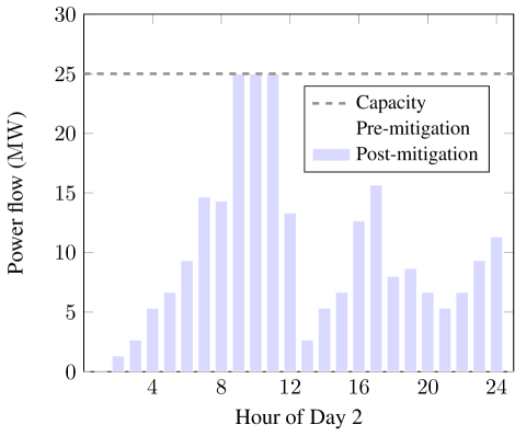
Figure 4: 3-bus case study: Congestion mitigation on Line 2–3.

V Large-scale case study and demonstration

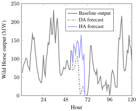
Figure 5: Wild Horse wind ramp.

To demonstrate the scalability of the framework, we developed a large-scale case study based on a realistic representation of the Pacific Northwest region of the United States. The system model, summarized in Table IX, was built from a subset of the WECC 2024 Common Case [32]. This production cost modeling data set projects how the generation mix of the Western Interconnection will change over time. The focal point of the case study was an actual $2\text{\,}\mathrm{MW}$/$1\text{\,}\mathrm{MWh}$ battery energy storage system located at SnoPUD’s Hardeson substation in Everett, WA. By itself, this amount of capacity is insufficient to significantly reduce transmission congestion; therefore, it was represented in the model as a $200\text{\,}\mathrm{MW}$/$100\text{\,}\mathrm{MWh}$ ESS. This served to better illustrate the capabilities of the coordination framework given adequate resources.

This case study examines a scenario in which there are substantial changes in the wind forecast between the day-ahead and hour-ahead frameworks. Specifically, we consider a multi-hour wind ramp at the Wild Horse wind farm ($273\text{\,}\mathrm{MW}$ capacity) near Ellensburg, WA. The day-ahead and hour-ahead wind power forecasts at Wild Horse are shown in Fig.​ 5. During this operating day, the $1.5$ mile Blue Lake–Troutdale $230\text{\,}\mathrm{kV}$ transmission line near Portland, OR is congested for roughly $11$ hours. That is, the solution to a standard unit commitment and economic dispatch causes violations of the short term line rating. Fig.​ 6 shows the real power flow on this line in both the pre- and post-mitigation stages.

The optimal net injections for the ESS are shown in Fig.​ 7. An action indicator value of $1$ implies the ESS is charging, and a value of $-1$ implies the ESS is discharging. The injections shown in Fig.​ 7 correspond to the two distinct blocks of time when the Blue Lake–Troutdale line is congested. Immediately prior to each congested period the battery is charged so that it may discharge at the correct moment to mitigate congestion. In conjunction with modestly redispatching some conventional generation units, this strategy is effective in satisfying the static system security constraints. A notable finding of this study is that the storage system was able to help mitigate congestion on a transmission line despite being roughly $170$ miles away.

In Fig.​ 7, the ESS injections determined in the day-ahead and hour-ahead frameworks do not fully overlap. In this case, the mismatch between the two is expected because of the substantial change in the system operating condition. Effectively, the solution provided by the day-ahead framework is no longer optimal because of the changes in the wind forecast. The hour-ahead framework allows TEPO to proactively plan for the wind ramp. The charging activity at the end of the day brings the ESS back to its target SOC, $E_{s}^{\prime}$.

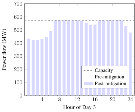
Figure 6: Congestion mitigation on Line 1716, Blue Lake–Troutdale 230 kV.

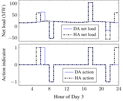
Figure 7: Net load at the SnoPUD energy storage bus.

TABLE IX: Large-scale test system information

Component	Quantity
Buses	$2,764$
Branches	$3,318$
Fixed generators	$440$
Controllable generators	$38$
Wind farms	$73$
Solar plants	$5$
Energy storage systems	$1$

V-A Demonstration

The framework presented in Sections II and III was implemented within SnoPUD’s production power scheduling environment. TEPO was implemented in GAMS using the IBM CPLEX solver [33, 34]. DEPO implements an OpenADR Virtual End Node that communicates with TEPO via a cloud-hosted XMPP server [22, 35]. Upon completion of the optimization procedure, DEPO supplies ESS scheduling recommendations to a human operator. The large-scale case study outlined above served as the basis for the live demonstration. To highlight the transmission-side impact, the ESS was not called upon for local service provision during the demonstration. Over the operating day with the wind ramp, the maximum absolute difference between the simulated and actual schedules was $70\text{\,}\mathrm{kW}$ for the $2\text{\,}\mathrm{MW}$ battery system. The scheduling differences largely reflect approximation errors in the SOC tracking constraints Eq. 43–Eq. 45.

VI Benchmark with one-shot optimization

Here we explore the possibility that, given sufficient centralized coordination, TEPO could solve a master problem encompassing all constraints and distribution system requirements. This hypothetical formulation would take the form of a one-shot optimization rather than a sequence of linked stages. The design of this master problem would need to carefully specify what information needs to be exchanged and when between TEPO and the DEPO instances. This one-shot formulation could potentially be decomposed preserving some degree of independence and information privacy by allowing each DEPO instance to solve its own subproblem. The complete development of a master problem that meets the above criteria is outside the scope of this paper; however, when the DEPOs make their storage capacity fully available to TEPO, as in the case study from Section V, the master problem effectively becomes a network-constrained unit commitment (NCUC) with energy storage constraints. Thus, we present a benchmark comparison of the operating costs incurred in Stage $4$ of the multistage framework versus the augmented NCUC, henceforth denoted as NCUC+. The purpose of this comparison is to provide a rough estimate of the cost of not solving the problem in a fully centralized manner.

VI-A Augmented network-constrained unit commitment

The tuple of decision variables in NCUC+ is

$$\xi:\mathopen{}\mathclose{{}\left(v_{i},y_{i},z_{i},\nu_{s},p_{ib},p_{i},p_{s}^{c},p_{s}^{d},x_{k},x_{w},\theta_{n}}\right),$$

where $p_{s}^{c}$ and $p_{s}^{d}$ are the charging and discharging schedules of the $s$th ESS, respectively. As in Eq. 37, $\nu_{s}$ is a binary variable that prevents simultaneous charging and discharging. The remaining decision variables are defined as in Stage $1$.

The objective function of NCUC+ is:

$$f(\xi)=\sum_{t\in\mathcal{T}}\sum_{i\in\mathcal{I}}C_{i}(t)+\sum_{t\in\mathcal{T}}\sum_{w\in\mathcal{W}}C_{w}(t)\\ +\sum_{t\in\mathcal{T}}\sum_{k\in\mathcal{K}}C_{k}(t)+\sum_{t\in\mathcal{T}}\sum_{s\in\mathcal{S}}C_{s}(t),$$ (50)

where $C_{i}$, $C_{w}$, and $C_{k}$ are defined as in Eq. 2. The energy storage utilization costs are

$$C_{s}(t)=m_{s}\mathopen{}\mathclose{{}\left[{p_{s}^{c}(t)+p_{s}^{d}(t)}}\right],$$ (51)

where charging and discharging are priced symmetrically for simplicity. In order to make a fair comparison, the incremental cost of storage utilization was set to match the incremental penalty on ESS injections from Eq. 27, i.e., ${m_{s}=\rho_{s}}$. The minimum operating cost objective in Eq. 50 results in the available storage capacity being used for a variety of transmission services, such as temporal arbitrage, rather than purely for congestion relief. The constraints of NCUC+ include those from Stage $4$ and a simplified energy storage model based on (35)–(45).

VI-B Quantitative comparison

TABLE X: Benchmark results summary

Problem	Storage cap.	Gen. cost	Cost reduction	Reduct. gap
	($\mathrm{MWh}$)	(k$)	($)	($\mathrm{\char 37\relax}$)
NCUC+	$0$	$1,740.93$	–	–
NCUC+	$100$	$1,735.96$	$4,964.27$	$0.0$
Stage $4$	$100$	$1,735.97$	$4,955.09$	$0.2$

The large-scale test system described in Section V was used for the benchmark comparison. As in the case study, the focal point of this analysis was operating day $3$. Each data point in the comparison corresponds to a scheduling method paired with a given amount of storage capacity. To determine a baseline, we ran NCUC+ with no energy storage. When there is no storage in the system, NCUC+ is mathematically equivalent to Stage $4$, i.e., they return exactly the same solution. Then the $200\text{\,}\mathrm{MW}$/$100\text{\,}\mathrm{MWh}$ battery was reinserted and the multistage and one-shot frameworks were compared. For all optimization runs, a relative MILP gap of $0.1\text{\,}\mathrm{\char 37\relax}$ was used as the stopping criterion, i.e., optcr=0.001 in GAMS. The results are summarized in Table X.

For the case with no energy storage, the generation costs are $1,740,926\text{\,}\mathrm{[}$$] over the day of interest. With the battery in the system, the generation costs incurred by NCUC+ are reduced by $4,964.27\text{\,}\mathrm{[}$$]. This difference is attributable to the ESS, which NCUC+ uses to perform a variety of transmission-side services. In contrast, the generation costs incurred in Stage $4$ of the multistage framework decrease by $4,955.09\text{\,}\mathrm{[}$$] in relation to the case with no storage. Although the reduction in operating cost is slightly smaller than with NCUC+, the difference is only about $0.2\text{\,}\mathrm{\char 37\relax}$. This difference, indicated in Table X as the cost reduction gap, can be partially attributed to the fact that the one-shot formulation uses the ESS to perform multiple transmission-side services while the multistage framework does not. The cost reduction gap is sensitive to the incremental penalties employed in the congestion relief stages. For instance, if the incremental penalty on wind curtailment is set much lower than the actual incremental cost, i.e., ${\rho_{w}\ll m_{w}}$, the congestion relief stages may produce storage injection schedules that presume too much wind curtailment and therefore have a larger gap. In this analysis, the incremental penalties were set to reflect the actual costs, e.g., ${\rho_{w}=m_{w}}$.

From an economic perspective, the cost reduction gap is indicative of how the social welfare declines when TEPO and DEPO act in their own self-interest. This benchmark comparison indicates that there is indeed a price to be paid for allowing TEPO and DEPO to act independently, but that price appears to be small when the incremental penalties in Stages $2$ and $3$ are set appropriately. Eliminating this effect entirely would require full centralized coordination and/or a carefully crafted decomposition of a suitable master problem.

VII Conclusion

This paper addresses the problem of how to share energy storage capacity among transmission and distribution entities. It describes and demonstrates a method for coordinating transmission-level congestion relief with local, distribution-level services in systems that lack centralized markets. A weighted ${\ell_{1}\text{-norm}}$ objective determines a minimal set of corrective actions required to alleviate transmission congestion. This work could be readily extended to accommodate other system-wide objectives, such as frequency regulation. Future work will explore the effect of line losses when sharing energy storage capacity among transmission and distribution entities. Finally, another interesting avenue of research will be the use of mathematical decomposition techniques (e.g., Dantzig-Wolfe decomposition) to analyze the coordination of energy storage services between transmission and distribution within a centralized environment.

Ryan Elliott is a Ph.D. candidate in the Department of Electrical Engineering at the University of Washington. His research focuses on renewable energy integration, wide-area measurement systems, and power system operation and control. Prior to pursuing a Ph.D., he was with the Electric Power Systems Research Department at Sandia National Laboratories from 2012–2015. While at Sandia, he served on the WECC Renewable Energy Modeling Task Force, leading the development of the WECC model validation guideline for central-station PV plants. In 2017, he earned an R&D 100 Award for his contributions to the design of a real-time damping control system using PMU feedback. Ryan received the M.S.E.E. degree from the University of Washington in 2012.

Ricardo Fernández-Blanco is a Postdoctoral Researcher at the University of Malaga, Spain. His research interests include the fields of operations and economics of power systems, smart grids, bilevel programming, hydrothermal coordination, electricity markets, and the water-energy nexus. Previously, he was a Postdoctoral Researcher at the University of Washington, Seattle, WA, USA, and later a Scientific/Technical Project Officer in the Knowledge for the Energy Union Unit at the Joint Research Centre (DG JRC) of the European Commission, Petten, The Netherlands. Ricardo received the Ingeniero Industrial degree and the Ph.D. degree in electrical engineering from the Universidad de Castilla-La Mancha, Ciudad Real, Spain, in 2009 and 2014, respectively.

Kelly Kozdras is the Distributed Energy Resource Planner at Puget Sound Energy (PSE). Previously while at PSE she provided engineering services for PSE-owned generating facilities and pilot projects in utility and customer-scale battery storage. She earned her M.S.E.E. degree from University of Washington in 2016, completing her thesis on modeling and analysis of a microgrid containing hydro and battery storage. Prior to that, Kelly worked in various capacities as an electrical engineer and task manager on infrastructure projects around the USA as well as at South Pole Station, Antarctica. She earned a B.S.E.E. from Rose-Hulman Institute of Technology in 1999, and is a licensed professional engineer in the state of Washington.

Josh Kaplan is an aspiring carpenter and avid outdoorsman based in Seattle, WA. Formerly, he was a founding employee of 1Energy Systems, an energy storage software company. At 1Energy, which became Doosan GridTech following acquisition, he was responsible for software design and project management on several energy storage deployments and research projects. Prior to his work in the energy storage field, he worked as a software engineer at Microsoft, primarily on developer tools products. Josh holds a B.A. degree in Political Science from the University of Washington.

Brian Lockyear is a Principal Software Development Engineer with Doosan GridTech. His interests include green energy in both design and implementation and in applications of artificial intelligence in energy control systems. He holds a Ph.D. in computer science from the University of Washington, a M.Arch. from the University of Oregon, and a B.S.E.E. from Oregon State University. Prior to Doosan, he worked for Synopsys, Tera Computer, and NASA.

Jason Zyskowski is the Senior Manager of Planning, Engineering and Technical Services at the Snohomish County PUD. He was the project manager for the District’s first energy storage system deployment and has contributed to numerous renewable generation and automation upgrade projects. Jason has been with the PUD since receiving the B.S.E.E. degree from the University of Washington in 2004. His professional experience includes time in the Transmission, System Protection and Substation Engineering departments. He is a registered professional engineer in the state of Washington.

Daniel Kirschen is the Donald W. and Ruth Mary Close Professor of Electrical Engineering at the University of Washington. His research focuses on the integration of renewable energy sources in the grid, power system economics and power system resilience. Prior to joining the University of Washington, he taught for 16 years at The University of Manchester (UK). Before becoming an academic, he worked for Control Data and Siemens on the development of application software for utility control centers. He holds a Ph.D. from the University of Wisconsin-Madison and an Electro-Mechanical Engineering degree from the Free University of Brussels (Belgium). He is the author of two books.

References

- [1] B. F. Hobbs and F. A. M. Rijkers, “Strategic generation with conjectured transmission price responses in a mixed transmission pricing system – Part I: Formulation,” IEEE Trans. Power Syst., vol. 19, no. 2, pp. 707–717, May 2004.
- [2] F. Teng and G. Strbac, “Business cases for energy storage with multiple service provision,” J. Modern Power Syst. and Clean Energy, vol. 4, no. 4, pp. 615–625, Oct. 2016.
- [3] X. He, R. Lecomte, A. Nekrassov, E. Delarue, and E. Mercier, “Compressed air energy storage multi-stream value assessment on the French energy market,” in 2011 IEEE Trondheim PowerTech, Jun., pp. 1–6.
- [4] W. Hu, P. Wang, and H. B. Gooi, “Assessing the economics of customer-sited multi-use energy storage,” in 2016 IEEE Region 10 Conf. (TENCON), Nov., pp. 651–654.
- [5] G. Fong, R. Moreira, and G. Strbac, “Economic analysis of energy storage business models,” in 2017 IEEE Manchester PowerTech, Jun., pp. 1–6.
- [6] O. Mégel, J. L. Mathieu, and G. Andersson, “Scheduling distributed energy storage units to provide multiple services under forecast error,” Int. J. Electr. Power and Energy Syst., vol. 72, pp. 48–57, 2015.
- [7] S. You, C. Træholt, and B. Poulsen, “Economic dispatch of electric energy storage with multi-service provision,” in 2010 Conf. Proc. Int. Power Eng. (IPEC), Oct., pp. 525–531.
- [8] J. M. Gantz, S. M. Amin, and A. M. Giacomoni, “Optimal capacity partitioning of multi-use customer-premise energy storage systems,” IEEE Trans. Smart Grid, vol. 5, no. 3, pp. 1292–1299, May 2014.
- [9] W. W. Kim, J. S. Shin, and J. O. Kim, “Operation strategy of multi-energy storage system for ancillary service,” IEEE Trans. Power Syst., vol. PP, no. 99, pp. 1–1, 2017.
- [10] K. Paridari, A. Parisio, H. Sandberg, and K. H. Johansson, “Demand response for aggregated residential consumers with energy storage sharing,” in 2015 IEEE Conf. Decision and Control (CDC), Dec., pp. 2024–2030.
- [11] W. Tushar, B. Chai, C. Yuen, S. Huang, D. B. Smith, H. V. Poor, and Z. Yang, “Energy storage sharing in smart grid: A modified auction-based approach,” IEEE Trans. Smart Grid, vol. 7, no. 3, pp. 1462–1475, May 2016.
- [12] J. Yao and P. Venkitasubramaniam, “Stochastic games of end-user energy storage sharing,” in 2016 IEEE Conf. Decision and Control (CDC), Dec., pp. 4965–4972.
- [13] D. Kalathil, C. Wu, K. Poolla, and P. Varaiya, “The sharing economy for the electricity storage,” IEEE Trans. Smart Grid, pp. 1–1, 2018.
- [14] Z. Hu and W. T. Jewell, “Optimal power flow analysis of energy storage for congestion relief, emissions reduction, and cost savings,” in IEEE PES Power Syst. Conf. and Expo., Mar. 2011, pp. 1–8.
- [15] A. D. D. Rosso and S. W. Eckroad, “Energy storage for relief of transmission congestion,” IEEE Trans. Smart Grid, vol. 5, no. 2, pp. 1138–1146, Mar. 2014.
- [16] L. S. Vargas, G. Bustos-Turu, and F. Larraín, “Wind power curtailment and energy storage in transmission congestion management considering power plants ramp rates,” IEEE Trans. Power Syst., vol. 30, no. 5, pp. 2498–2506, Sep. 2015.
- [17] H. Khani, M. R. D. Zadeh, and A. H. Hajimiragha, “Transmission congestion relief using privately owned large-scale energy storage systems in a competitive electricity market,” IEEE Trans. Power Syst., vol. 31, no. 2, pp. 1449–1458, Mar. 2016.
- [18] G. Koeppel, M. Geidl, and G. Andersson, “Value of storage devices in congestion constrained distribution networks,” in 2004 Int. Conf. Power Syst. Tech. (PowerCon), vol. 1, Nov., pp. 624–629.
- [19] FERC, “Electric storage participation in markets operated by regional transmission organizations and independent system operators,” Notice of Proposed Rulemaking, Docket Nos. RM16-23-000; AD16-20-000, Nov. 2016.
- [20] CAISO, “Joint workshop report and framework: Multiple-use applications for energy storage,” CPUC Rulemaking 15-03-011, Available at http://docs.cpuc.ca.gov/PublishedDocs/Efile/G000/M187/K237/187237488.PDF, May 2017.
- [21] T. Samad, E. Koch, and P. Stluka, “Automated demand response for smart buildings and microgrids: The state of the practice and research challenges,” Proc. of the IEEE, vol. 104, no. 4, pp. 726–744, Apr. 2016.
- [22] C. McParland, “OpenADR open source toolkit: Developing open source software for the smart grid,” in 2011 IEEE Power and Energy Soc. General Meeting, Jul., pp. 1–7.
- [23] H. Pandžić, Y. Wang, T. Qiu, Y. Dvorkin, and D. S. Kirschen, “Near-optimal method for siting and sizing of distributed storage in a transmission network,” IEEE Trans. Power Syst., vol. 30, no. 5, pp. 2288–2300, Sep. 2015.
- [24] B. Stott, J. Jardim, and O. Alsaç, “DC power flow revisited,” IEEE Trans. Power Syst., vol. 24, no. 3, pp. 1290–1300, Aug. 2009.
- [25] A. J. Conejo, J. M. Arroyo, N. Alguacil, and A. L. Guijarro, “Transmission loss allocation: A comparison of different practical algorithms,” IEEE Trans. Power Syst., vol. 17, no. 3, pp. 571–576, Aug. 2002.
- [26] A. L. Motto, F. D. Galiana, A. J. Conejo, and J. M. Arroyo, “Network-constrained multiperiod auction for a pool-based electricity market,” IEEE Trans. Power Syst., vol. 17, no. 3, pp. 646–653, Aug. 2002.
- [27] G. M. Fung and O. L. Mangasarian, “Equivalence of minimal - and -norm solutions of linear equalities, inequalities and linear programs,” J. Optimization Theory and Appl., vol. 151, no. 1, pp. 1–10, Oct. 2011.
- [28] D. L. Donoho, “Compressed sensing,” IEEE Trans. Inf. Theory, vol. 52, no. 4, pp. 1289–1306, Apr. 2006.
- [29] D. L. Donoho and Y. Tsaig, “Fast solution of -norm minimization problems when the solution may be sparse,” IEEE Trans. Inf. Theory, vol. 54, no. 11, pp. 4789–4812, Nov. 2008.
- [30] M. A. T. Figueiredo, R. D. Nowak, and S. J. Wright, “Gradient projection for sparse reconstruction,” IEEE J. Sel. Topics Signal Process., vol. 1, no. 4, pp. 586–597, Dec. 2007.
- [31] O. L. Mangasarian, “Absolute value equation solution via linear programming,” J. Optimization Theory and Appl., vol. 161, no. 3, pp. 870–876, Jun. 2014.
- [32] WECC, “Release notes for WECC 2024 common case, v1.1,” Western Electric Coordinating Council report. Available at https://www.wecc.biz/Reliability/140815-2024CC-V1.1.zip, 2014.
- [33] R. Rosenthal, “GAMS – A user’s guide,” GAMS Development Corporation, Available at https://www.gams.com/24.8/docs/userguides/GAMSUsersGuide.pdf, Washington, DC, USA, May 2017.
- [34] G. Sander and A. Vasiliu, “Visualization and ILOG CPLEX,” in Proc. 12th Int. Conf. Graph Drawing. Berlin, Heidelberg: Springer-Verlag, 2004, pp. 510–511.
- [35] A. Hornsby and R. Walsh, “From instant messaging to cloud computing, an XMPP review,” in 2010 IEEE Int. Symp. Consumer Electron. (ISCE), Jun., pp. 1–6.