The effects of competition between random sequential nucleation of point-sized seeds and island growth by adsorption of finite-sized grains

Abstract

We study random sequential adsorption of particles from pool onto a one dimensional substrate following ballistic deposition rules, with separate nucleation and growth processes occurring simultaneously. Nucleation describes the formation of point-sized seeds, and after a seed is sown, it acts as an attractor and grows in size by the addition of grains of a fixed-sized. At each time step either an already-nucleated seed can increase in size, or a new seed may be nucleated. We incorporate a parameter $m$, to describe the relative rates of growth to nucleation. We solve the model analytically to obtain gap size distribution function and a general expression for the jamming coverage as a function of $m$. We show that the jamming coverage $\theta(m)$ reaches its maximum value $\theta(m)=1$ in the limit $m\rightarrow\infty$ following a power-law $\theta(\infty)-\theta(m)\sim m^{-1/2}$. We also perform extensive Monte Carlo simulation and find excellent agreement between analytic and numerical results.

I Introduction

The kinetics of a monolayer growth by surface adsorption, deposition of particles onto solid substrates, has been studied extensively over the last many decades ref.evans ; ref.tarjus ; ref.schaaf ; ref.bartelt_review ; ref.book_privman ; ref.schaaf_review . One of the reasons for this is that it finds applications that covers many topic in physics, chemistry, biology and other branches of science and technology. There are numerous examples, such as the adsorption of colloids, bacteria, protein or latex particles on solid surfaces, macromolecules on biological membranes, growth of atomic islands of metals or semiconductors, etc., which are of interest in science and technology ref.has1 ; ref-svs ; ref-svs2 ; ref.has2 ; ref.has3 ; ref.finegold ; ref.evans_surface . The development of a theoretical understanding of the kinetics of adsorption poses many fundamental challenges owing to its non-equilibrium nature which means that the well-developed formalism of equilibrium statistical physics cannot be applied. One of the litmus tests of the degree of its complexity is that one can hardly make any progress analytically in more than one dimension; most analytical work remains confined to one spatial dimension ref.quasi_1 ; ref.quasi_2 ; ref.quasi_3 . The simplest case of random sequential adsorption (RSA) process was that considered by Alfred Renyi in 1958 ref.renyi ; ref-gonz ; ref-hemmer , which is known as the ‘car parking’ problem, in which one-dimensional ‘cars’ of a unfiorm length $\sigma$ are ‘parked’ sequentially at random available positions in a car park of length $L\gg\sigma$. After a sufficiently long time, all remaining gaps are shorter than $\sigma$ and no further adsorption is possible, at which point the expected coverage is given by Renyi’s constant, $\theta_{\infty}=0.7475979...$. Typically RSA is considered as irreversible and particle-particle interactions are accounted for by not allowing overlaps. This minimalist model captures many generic features of deposition phenomena.

Many variants of the RSA model have been devised suits various special conditions occurring in real systems: for example, to model protein adsorption onto DNA, the case of binding with overlaps ref.em1 , and reversible binding ref.em2 have been analysed. In 1992 Talbot and Ricci proposed a ballistic deposition (BD) model to take into account of strong self-attraction effects. They assumed that when the particle is deposited on the substrate, rather than being stationary, it moves towards closest already adsorbed particle, increasing the size of that island ref.talbot ; ref.ps . The attempt is rejected only when it fails to reach the surface. In 1995, Pagonabarraga et al. proposed yet another variant, in which particle can reach the surface along an inclined direction ref.pagonabarraga . Later, the deposition of competitive binary mixture of finite sized particles was been considered ref.hassan_schimidt ; ref.hassan_kurths . The RSA of mixture of particles of different uniform sizes has been studied ref.hassan_mixture ; ref.lr1 . The RSA model in presence of precursor-layer diffusion and desorption has also been studied where accelerated RSA and growth-and-coalescence has been considered as a special case ref.filipe ; ref.filipe2 . An extension to two dimensional RSA was simulated by Purves et al. ref.lr2 . Recently, a variant of RSA to the adsorption of particles modelling mobile patches has been proposed motivated by the coverage of oil droplets by DNA-functionalized colloidal particles ref.mobole_patches . The shapes of the depositing particles has also been considered in one of the recent articles ref.Adrian_Baule . Besides, Subashiev et al. studied the RSA of shrinking or expanding particles ref.Subashiev

In this article, we propose a model that generalises RSA to describe two processes: (i) the nucleation of point-sized seeds and (ii) the growth by the addition fixed-sized grains. Our aim remains that of understanding the kinetics through which a monolayer is formed. However, the distinction between the rates of nucleation and growth may lead to dynamics which differ significantly from Renyi’s classic ‘car parking’ problem. In particular, we assume that in each time interval either a seed is sown or an already-sown seed grows. We include a tuning parameter, $m$, which regulates the rate of growth of existing domains relative to the nucleation of new sites.

We solve the model analytically to find an approximate expression for the coverage and for the jamming limit as a function of $m$. For large values of $m$ island growth dominates, through the frequent ballistic deposition of grains; whilst for small $m$, growth occurs at a relatively small rate, and the nucleation of fresh seeds is dominant. We also give an algorithm to simulate the model numerically. We find excellent agreement between our analytical and numerical results revealing that the proposed integro-differential equation of the model accurately describes the behaviour of the algorithm. We show that the jamming coverage reaches the maximum jamming coverage $\theta(m)\rightarrow 1$ in the limit $m\rightarrow\infty$ following a power-law $\theta(m)\sim 1-m^{-1/2}$.

The paper is organized as follows: in Sec. II, the model is introduced and the algorithm for simulating it is described. Sec. III, contains a theoretical approach to solving the model to find the gap size distribution function and the behaviour in the jamming limit. Numerical results are presented in IV alongside a comparison with the analytical solutions. The results are discussed and conclusions drawn in Sec. V.

II Definition of the model

Figure 1: Schematic description of the processes occurring in our model at the global scale; random sequential nucleation of seeds is shown on the right, and island growth deposition of a grain of positive size in the centre.

We introduce a new class of RSA which consists of two processes: firstly, nucleation—in which a point-sized seed is deposited in a gap on a substrate, and subsequently, growth—through which the island domains grow by the deposition of a grain of a positive size. Only one such event can occur in each time interval. The nucleation step is identical to classic RSA in that it occurs randomly, at any point in a gap, with equal probability. The deviation from RSA is that the seeds have zero size. Growth occurs through the deposition of domains of finite size $\sigma>0$, as in RSA, though these are only deposited ballistically - so that they are adjacent to an existing domain (whereas in RSA, deposition is typically at a randomly-determined location in a gap). Any attempt to deposit a seed or a grain on an existing island is ignored.

Figure 2: Illustration of the quantities involved in one deposition event in our model.

The islands thus have sizes which increase from zero (for a newly nucleated domain) in steps of $\sigma$ with the only upper bound being the size of the substrate simulated. The length of a gap is defined by the difference in locations of its ends, whether these are a seed, a large island, or the end of the domain.

The only quantity we have yet to specify is the relative frequency of growth (deposition of $\sigma$-sized block) to nucleation (seed deposition). We denote this my $m$ so that when $m>1$ growth dominates and for $m<1$ nucleation occurs more frequently. These processes are illustrated in Fig. 1. The process may be simpler to understand by giving the algorithm used in our simulations. We start with a single empty substrate of length $L\gg 1$, that is, a single gap. Commentary on the effect of steps is given in slanted text.

• Generate a random number, $R_{1}$, from a uniform distribution on the interval $(0,L)$.

• If $R_{1}$ falls in a gap, let $X$ be the location of the left-hand edge of gap, and $Y$ be the length of the gap. If $R_{1}$ falls on an existing island, go to step (iv).

  This method of choosing points for deposition means that larger gaps are chosen preferentially.

  The role of $R_{1}$ is simply to choose a gap in which to deposit a particle, we next determine what is deposited in the gap and where it is deposited.

• Determine whether nucleation or growth occurs:
  In place of the gap which actually occupies the interval $(X,X+Y)$, consider the gap as being the larger interval $(X-m\sigma,X+Y+m\sigma)$.

  Let $R_{2}$ be a random variable taken from a uniform distribution on the interval $(X-m\sigma,X+Y+m\sigma)$.

  A gap can be terminated by two seeds, two grains or a grain and a seed (or in the two cases $x=0$ and $x=L$, the end of the domain and either a seed or a gap): how a gap is terminated has no influence on what deposition processes occur in the gap.

  (iii.a)

  If $X-m\sigma<R_{2}<X$ then deposit grain of size $\sigma$ in the location $(X,X+\sigma)$; the effect of this is to reduce the gap from the interval $(X,X+Y)$ to $(X+\sigma,X+Y)$. This constitutes growth the left island by ballistic deposition of a grain of size $\sigma$.

  (iii.b)

  If $X<R_{2}<X+Y$ then deposit a seed nucleus (size zero) at $x=R_{2}$ the effect of this is to replace the gap on the interval $(X,X+Y)$ with two gaps, which are given by the intervals $(X,R_{2})$ and $(R_{2},X+Y)$. This constitutes random sequential nucleation of a zero-sized seed.

  (iii.c)

  If $X+Y<R_{2}<X+Y+m\sigma$ then deposit grain of size $\sigma$ in the location $(X+Y-\sigma,X+Y)$; the effect of this is to reduce the gap from the interval $(X,X+Y)$ to $(X,X+Y-\sigma)$. This constitutes growth of the right island by ballistic deposition of a grain of size $\sigma$.

  The effect of this is that probability of nucleation in this gap is $Y/(Y\!+\!2m\sigma)$ and the probability of growth in this gap is $2m\sigma/(Y\!+\!2m\sigma)$ so the relative rate of growth to nucleation is $2m\sigma/Y$.

  The effect of large values of $m$ is to make island growth by deposition of grains occur at a faster rate relative to nucleation of fresh seeds; and, conversely, the effect of small $m$ is to make growth occur at a slower rate, thus favouring nucleation. The quantity $m$ can be viewed as a relative rate parameter.

  The reason we describing grain deposition as ballistic, is that we assume the grain, once deposited on the substrate is mobile, and is attracted to the already-deposited grains, thus it moves to the closest endpoint (whether grain or seed) and stops moving when it comes into contact with a grain or a seed.

• Increase time by one and repeat from (i). It is important to increase time even when the attempt at deposition fails, since we are interested in the dynamics of the process, and how it slows at later times.

III Analytical approach

III.1 Derivation of mean field model

To solve the model analytically, we need to appreciate the fact that the random sequential nucleation of point-sized seeds is equivalent to binary fragmentation of gaps. Placing a seed in a gap divides a gap of size $x$ into two smaller gaps, one of size $y$ and the other of size $x-y$ (with $0<y<x$). In general, binary fragmentation is described by the equation

$$\frac{\partial c(x,t)}{\partial t} = -c(x,t)\int_{0}^{x}F(y,x-y)\,\mbox{d}y$$

$$+2\int_{x}^{\infty}F(x,y-x)c(y,t)\,\mbox{d}y,$$

where $c(x,t)$ denotes the expected number of gaps of length $x$ at time $t$. The first term on the right hand side of (III.1) describes the rate at which a particle (gap) of size $x$ is divided into two particles of size $y$ and $x-y$, and the second term describes a particle of size $y\geq x$ breaks into two smaller particles of sizes $x$ and $y-x$ ref.krapivsky_redner_naim . The choice of the kernel $F(x,y)$ describes the rate at which the particles fragment. The case $F(x,y)=1$ is known as Yule-Furry process ref.Bhabha , or a random scission process ref.Jellinek . The corresponding rate equation for the random sequential nucleation of point-sized seeds is therefore

$$\frac{\partial c(x,t)}{\partial t}=-xc(x,t)+2\int_{x}^{\infty}c(y,t)\,\mbox{d}y,$$ (2)

where $c(x,t)$ is the gap size distribution function.

To describe the creation of a gap of size $x$ due to growth of an island into a gap of size $x+\sigma$ we add a term of the form $2m\sigma c(x+\sigma,t)$. Gaps of size $x$ are also destroyed due to growth of islands on both sides, so it is described by $2m\sigma c(x,t)$. Thus, the governing equation for $c(x,t)$ for random sequential nucleation and growth is given by the integro-differential equation

$$\frac{\partial c(x,t)}{\partial t} = -xc(x,t)+2\int_{x}^{\infty}c(y,t)\,\mbox{d}y$$

$$+2m\sigma c(x+\sigma,t)-2m\sigma c(x,t),$$

$$\hskip 85.35826pt\mbox{(for $x\geq\sigma$)},$$

$$\frac{\partial c(x,t)}{\partial t} = -xc(x,t)+2\int_{x}^{\infty}c(y,t)\,\mbox{d}y$$ (4)

$$+2m\sigma c(x+\sigma,t),\qquad\mbox{(for $x<\sigma$)}.$$

Note that each gap is either bordered by a grain or by a seed. The factor $m$ is added as tuning parameter that tunes the strength of attraction for growth of grain. This model describes the expected value of the stochastic algorithm given in Section II. Typically, there will be fluctuations, and the mean field results obtained by taking the average over many realisations of the algorithm.

III.2 Special case of the mean field model

Combining (III.1) and (4), we obtain

$$\frac{\partial c}{\partial t} = -xc(x,t)+2\int_{x}^{\infty}c(y,t)\,\mbox{d}y$$

$$+2m\sigma c(x+\sigma,t)-2m\sigma c(x,t)H(x-\sigma).$$

In the limit $\sigma\rightarrow 0^{+}$ we obtain

$$\frac{\partial c}{\partial t}=-xc(x,t)+2\int_{x}^{\infty}c(y,t)\,\mbox{d}y+2\mu\frac{\partial c}{\partial x},$$ (6)

where $\mu=m\sigma^{2}$.

The equation (6) can be solved by use of Laplace transforms, since

$$\overline{c}(s,t) = \int_{0}^{\infty}c(x,t){\rm e}^{-sx}\,\mbox{d}x,$$ (7)

$$c(0,t) = \lim_{s\rightarrow\infty}s\overline{c}(s,t),$$ (8)

imply that (6) can be rewritten as

$$\frac{\partial\overline{c}}{\partial t} = \frac{\partial\overline{c}}{\partial s}+\frac{2}{s}\left(\overline{c}(0,t)-\overline{c}(s,t)\right)+2\mu s\overline{c}(s,t)$$ (9)

$$-2\mu\lim_{\widehat{s}\rightarrow+\infty}\widehat{s}\,\overline{c}(\widehat{s},t).$$

If we assume $\overline{c}(s,t)$ is a rational polynomial, namely $\overline{c}(s,t)=A(t)/(s+B(t))$, then we find

$$\frac{\mbox{d}B}{\mbox{d}t}=1, \frac{1}{A}\frac{\mbox{d}A}{\mbox{d}t}=\frac{2}{B}-2\mu B,$$ (10)

hence

$$B(t) = t+\beta,$$ (11)

$$A(t) = \alpha(t+\beta)^{2}{\rm e}^{-\mu t^{2}-2\mu\beta t},$$ (12)

where $\alpha,\beta$ are arbitrary constants.

In the case of $\sigma\rightarrow 0^{+}$, the total coverage $\theta(t)=1-\int_{0}^{\infty}xc(x,t)\,\mbox{d}x$ is of course unity in the large time limit (that is, $\theta\rightarrow 1^{-}$ as $t\rightarrow+\infty$), but the kinetics by which this limit is approached is complicated, being given by

$$1-\theta(t) = \frac{1}{L}\int_{0}^{L}x\,c(x,t)\,\mbox{d}x$$ (13)

$$= \frac{A(t)}{B(t)^{2}}=\alpha\,{\rm e}^{-\mu t^{2}-2\mu\beta t}.$$

Typically, this decay is extremely rapid (${\rm e}^{-\mu t^{2}}$); however, if $\mu$ were small then an intermediate timescale, where $1-\theta(t)\sim O(1/t)$, could be observed; and if $\beta$ were large whilst $\mu$ small, then exponential decay might be seen ($1-\theta(t)\sim{\rm e}^{-\mu\beta t}$). In the case $\beta=0$ this simplifies a little, to $B=t$, $A=\alpha t{\rm e}^{-\mu t^{2}}$ and $1-\theta(t)=\alpha{\rm e}^{-\mu t^{2}}$.

The form of the resulting solution of (6)

$$c(x,t)=A(t){\rm e}^{-xB(t)},$$ (14)

motivates the use of this formula as an ansatz for the solution of the more general problem (III.1)–(4) in which $\sigma>0$ and where we are interested in the solution at $\mathcal{O}(1)$ times. Dimensional analysis ($c_{t}\sim-xc$) implies that the gap size $x$ has the units of inverse time, thus $B(t)$ should have units of time so that the argument of the exponential function is dimensionless. Therefore we assume $B(t)\sim t$, taking $\beta=0$ since we do not expect the gap length distribution to be exponential at $t=0$.

In order to obtain exact solutions for $A(t)$ we substitute the ansatz (14) into the rate equation (III.1) for $x>\sigma$, which (following application of $\mbox{d}B/\mbox{d}t=1$) gives the differential equation

$$\frac{\mbox{d}\ln A}{\mbox{d}t}=\frac{2}{t}-2m\sigma(1-e^{-\sigma t}),$$ (15)

for $A(t)$, whereupon $A(t)$ is given by

$$A(t)=A_{0}t^{2}\exp(-2m\sigma t+2m\sigma(1-e^{-\sigma t})).$$ (16)

III.3 Solution of mean field model at early times

The integro-differential equation (III.1) should be solved subject to the initial data

$$c(x,0)=\delta(x-L),\qquad\mbox{with $L\gg 1$},$$ (17)

where $L$ is the length of the substrate. If we define moments of the distribution $c(x,t)$ by

$$I_{n}(t)=\int_{0}^{\infty}x^{n}c(x,t)\,\mbox{d}x,$$ (18)

then the initial conditions (17) imply

$$I_{0}(0)=1,\qquad I_{1}(0)=L.$$ (19)

However, given the ansatz (14) we have

$$I_{0}(t)=\frac{A(t)}{B(t)},\qquad I_{1}(t)=\frac{A(t)}{B(t)^{2}},$$ (20)

thus for $t=0$ we have $B(0)=\beta$ and $A(0)=\beta^{2}$ giving $I_{0}(0)=\beta$ and $I_{1}(0)=\beta^{2}$.

This apparent contradiction between the initial conditions (17) and the ansatz (14) with (16) lies in considering an early time asymptotic analysis of the system. At early times, since the substrate is almost entirely empty, there are a few gaps, gaps are typically large, and nucleation dominates growth, thus we have $I_{0}=\mathcal{O}(1)$ and $I_{1}=\mathcal{O}(L)$. In this early time regime, we note that the gap shrinkage due to growth, $\sigma$, is infinitesimally small in comparison with the size of gaps, that is $\sigma\ll L$, and thus we approximate the dynamics of the system (III.2) by (6). By integrating, we note that, to leading order, we have

$$\frac{\mbox{d}I_{0}}{\mbox{d}t}=I_{1}-2\mu c(0,t),\qquad\frac{\mbox{d}I_{1}}{\mbox{d}t}=-2\mu I_{0},$$ (21)

together with (19). Thus, at early times, we have

$$I_{0}=\overline{c}(0,t)\sim 1+Lt,\qquad I_{1}\sim L-2\mu t.$$ (22)

Introducing the rescaling

$$\tau=Lt,\qquad q=sL,$$ (23)

with $\overline{c}(p,0)={\rm e}^{-Lp}$ and $G(q,\tau)=\overline{c}(p,t)$, we rewrite the governing equation (9)

$$p\frac{\partial\overline{c}}{\partial t}-p\frac{\partial\overline{c}}{\partial p}=2(\mu p^{2}-1)\overline{c}+2I_{0}(t)-2p\mu c(0,t),$$ (24)

at leading order, as

$$q\frac{\partial G}{\partial\tau}-q\frac{\partial G}{\partial q}=2(1+\tau-G),$$ (25)

with $G(q,0)={\rm e}^{-q}$. This can be solved by the method of characteristics, (giving ${\rm e}^{u}=1+\tau/q$ and $r=q+\tau$) which gives the solution

$$G(q,\tau) = (1\!+\!\tau\!-\!q)+(q\!+\!\tau\!-\!1+{\rm e}^{-q-\tau})\left(\frac{q}{q\!+\!\tau}\right)^{2}.$$

Inverting the transformations (23), we find

$$\overline{c}(s,t)=\frac{Lt^{2}}{s+t}+\frac{t^{2}+2ts}{(t+s)^{2}}+\frac{s^{2}{\rm e}^{-Ls-Lt}}{(s+t)^{2}},$$ (27)

which implies

$$c(x,t) \sim Lt^{2}{\rm e}^{-xt}+(2-xt)t{\rm e}^{-xt}$$

$$+H(x\!-\!L)[{\rm e}^{-Lt}\delta(x\!-\!L)+t{\rm e}^{-xt}(xt\!-\!Lt\!-\!2)].$$

Here, the leading order term, $c(x,t)\sim Lt^{2}{\rm e}^{-xt}$ implies $A(t)\sim Lt^{2}$ for $t\ll 1$, so the constant $A_{0}$ in (16) should be given by $A_{0}=L$. Solving (15) for $A(t)$ subject to this matching condition gives

$$A(t)=Lt^{2}e^{-2m\sigma t+2m\sigma(1-e^{-\sigma t})}.$$ (29)

The asymptotic solution of Eq. (III.1) is therefore

$$c(x,t)=Lt^{2}e^{2m(1-e^{-\sigma t})}{\rm e}^{-(x+2m\sigma)t}\hskip 8.53581pt{\rm for}\hskip 8.53581ptx\geq\sigma.$$ (30)

The above solution implies that we can still recover the solution of the binary fragmentation process by taking $\sigma=0$ ref.krapivsky_redner_naim . It is important to mention that the solution for $c(x,t)$ alone is enough to provide us with all the interesting information that we need.

III.4 Behaviour of the coverage

One of the most important quantities of interest in the process of RSA is the coverage, which is defined by

$$\theta(t;m)=1-\frac{1}{L}\int_{0}^{L}x\,c(x,t)\,\mbox{d}x.$$ (31)

Denoting the units or dimensions of a term by $[\cdot]$, and considering the terms in Eq. (III.2), we note that $[x]=1/[t]$, which is consistent with the term ${\rm e}^{xt}$ in (III.3). Furthermore, since $L$ is length of the substrate, we have $[L]=[x]$, and $[\int xc(x,t)\,\mbox{d}x]=[x]$, thus $[c]=[x]^{-1}=[t]$, which is consistent with the prefactor on the right-hand side of Eq. (30).

Equation (31) describes the fraction of substrate covered by deposited particles ($\theta$ being dimensionless). In the classic ‘car parking’ case of RSA only 74.759 % of the total substrate is covered. We now investigate how the ballistic deposition of particles with random sequential nucleation changes the jammed state and kinetics of jamming.

In the present case there is always space for nucleation as the seeds do not have any width (by definition). Seeds do not directly contribute to the coverage; however, they influence the jamming kinetics, since the presence of multiple nuclei within $\sigma$ of each other prevent the deposition of grains and reduce the rate of island growth.

In this model the jamming coverage is the state when there are no more gaps available for the growth of particles of size $\sigma$. Once this state is achieved, it is no longer necessary to continue considering the process of nucleation since the coverage can no longer change.

FIG 3

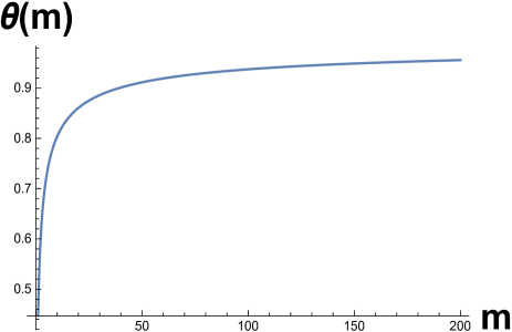
(a)

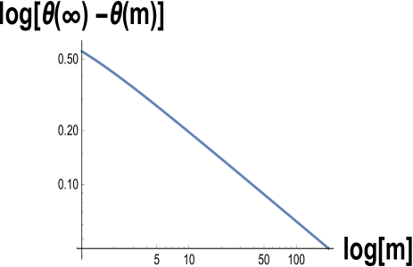
(b)

Figure 3: (a) We show how $\theta(m)$ varies with $m$. (b) We plot $\log[\theta(\infty)-\theta(m)]$ versus $\log[m]$ and find perfectly straight line with slope almost equal to $1/2$ only if we choose $\theta(\infty)=1$, implying that the jamming coverage $\theta(m)$ reaches its maximum value of $\theta(m)=1$ following a power-law $\theta(m)\sim 1-m^{1/2}$.

It is interesting to determine how the kinetics of jamming differs in this model from that of standard RSA. To find the jamming coverage, it is more convenient to consider the rate equation for the coverage rather than the coverage itself. We differentiate the definition of $\theta$ with respect to time $t$, giving

$$\frac{\mbox{d}\theta}{\mbox{d}t} = -\frac{1}{L}\int_{0}^{\infty}x\frac{\partial c(x,t)}{\partial t}\,\mbox{d}x,$$

$$= -\frac{1}{L}\int_{0}^{\sigma}x\frac{\partial c(x,t)}{\partial t}\,\mbox{d}x-\frac{1}{L}\int_{\sigma}^{\infty}x\frac{\partial c(x,t)}{\partial t}\,\mbox{d}x.$$

In the first term we substitute the rate equation for $x<\sigma$ and in the second term we substitute the rate equation for $x\geq\sigma$. Thus

$$\frac{\mbox{d}\theta}{\mbox{d}t}=\frac{2m\sigma^{2}}{L}\int_{\sigma}^{\infty}c(x,t)\,\mbox{d}x.$$ (33)

This equation shows that only the finite-sized particles contribute to the coverage, and the lower limit of $\sigma$ since only gaps of size above $\sigma$ can be filled. The right hand side of Eq. (33) bears the dimension of inverse time, as it should. Since $\theta(t,m)|_{t=0}=0$, by (14) and (29) we find

$$\theta(t,m)=2m\int_{0}^{\sigma t}s\exp\left(2m(1-e^{-s})-(2m+1)s\right)\,\mbox{d}s,$$ (34)

and hence

$$\theta(\infty,m)=2m\int_{0}^{\infty}s\exp\left(2m(1-e^{-s})-(2m+1)s\right)\,\mbox{d}s.$$ (35)

Since $\theta$ is a dimensionless quantity and, in the limit of large substrate length $L$, the only length in the system is $\sigma$, thus the final coverage should be independent of $\sigma$ –a non-trivial and interesting result. In Fig. 3a we plot the analytical solution for jamming coverage given by (35) to show how the jamming coverage $\theta(m)$ varies with the strength of attraction $m$.

To further quantify how the coverage $\theta$ depends on $m$, we plot $\log[\theta(t;m)|_{t\rightarrow\infty,m\rightarrow\infty}-\theta(t;m)_{t\rightarrow\infty}]$ against $\log(m)$ in Fig. 3b, finding a straight line. We only find a perfect straight line if we choose $\theta(\infty;m)|_{m\rightarrow\infty}=1$, and then the slope is equal to $1/2$. This implies that $\theta(\infty;m)$ approaches $\theta(\infty,m)_{m\rightarrow\infty}=1$ following the power-law $\theta(\infty,m)=1-m^{-1/2}$ for all $m$.

IV Numerical Simulation

Here we address the questions such as ‘what are the dynamics of the process?’, ‘what is the effect of the tuning parameter $m$?’ Our goal is to verify and illustrate the theoretical results through numerical simulations of the nucleation and growth algorithm to show that the model is well understood.

The simulations are restricted to a substrate of finite length, $L$. For sufficiently large $L$ (compared to the grain size, that is, $L\gg\sigma$) the effects of finite size $L$ are negligible. We follow the algorithmic steps (i)—(iv) given in Section II which are also illustrated in Fig. 2. The time scale in the simulations is given by the number of attempts to nucleate a seed or to grow a grain, regardless of whether the attempt is successful or not. Using this time scale and expressing all lengths in terms of $\sigma$, the simulation results can be directly compared to the solution of the rate equations (III.1)–(4) and the solution for the jamming limit (35).

To test the analytic solution for $c(x,t)$ of the rate equation (III.1)–(4) given by (30), we need to choose a value for $m$ (eg $m=1$), perform a simulation until no further island growth is possible, and then extract the sizes of all gaps from the simulation at a range of times, $t$. The distribution of gap sizes can then be constructed.

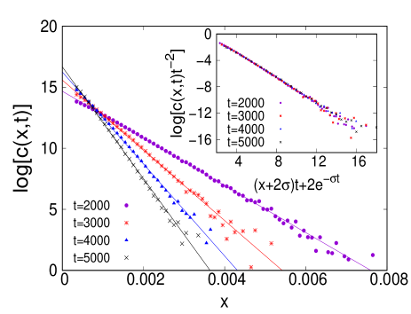
(a)

Figure 4: Plots of the gap size distribution function $c(x,t)$ against $x$ shown on a $\log$-linear scale using ensemble averaged data for three different times. The inset shows the same data, but with $\log[c(x,t)/Lt^{2}$ plotted against $(x+\sigma)t+2e^{-\sigma t}$ to show that the data collapses only a universal line.

This histogram data in which height represents the number of gaps within a given range of gap sizes (say of width $\Delta x$), normalized so that area under curve gives the number of gaps present in the system at time $t$ regardless of their sizes. Such data is shown in Figs. 4, on a $\log$-linear scale so that the extremely small frequency of large gaps remains visible. Plotting the data at a range of times clearly shows a family of straight lines with time-dependent gradients and intercepts, indicating the distribution is exponential in $x$.

(a)

Figure 5: Plots of the jamming coverage $\theta(\infty;m)$ against $m$, clearly showing that as the strength of attraction ($m$) increases, the corresponding coverage increases sharply to its maximum value $\theta(\infty;m)_{m\rightarrow\infty})\rightarrow 1$.

For further verification in the inset of Fig. 4 we plot $\log[c(x,t)/Lt^{2}$ against $(x+2\sigma)t+2e^{-\sigma t}$ and find that all the data points at all times collapse onto a single straight line. This is a strong confirmation of the theory of Section III, and (30) in particular. The inset of Fig. 4 confirms that the universal distribution is exponential.

The coverage in the jamming limit is one of the most interesting properties of generalised RSA processes. We find that the jamming coverage increases with the relative growth rate, $m$, as expected; this is shown in Fig. 5. In the limit $m\rightarrow\infty$, the jamming coverage approaches the maximum value of $\theta=1$. Comparing Figs. 5 and 3, we find an excellent agreement between simulation and theory. To determine how the jamming coverage $\theta(\infty,m)$ depends on $m$, we plot $\log(\theta(\infty;m)|_{m\rightarrow\infty}-\theta(\infty;m)$ against $\log(m)$ in the inset of Fig. 5 and find a straight line. It is noteworthy that the final coverage is described by a formula as simple as $\theta=1-m^{-1/2}$.

V Discussion and Conclusions

In this article, we have studied formation of monolayer through the nucleation of point-sized particles and the subsequent growth by fixed-sized grains. We have assumed that deposited domains, or ’islands’ act as attractors for grains (via ballistic deposition) and so increase in size, simultaneously with the nucleation of fresh sites by deposition at random vacant locations. As well as the size of the grains through which growth occurs ($\sigma$), we have also incorporated a parameter $m$ to control the strength of the attraction by increasing the apparent size of the seed or grain.

From the algorithm we have derived an integro-differential equation which predicts the mean behaviour of the stochastic process. We have solved this model analytically determining an ansatz for the gap size distribution function (14) and hence an expression for the jamming coverage $\theta(m)$. Remarkably, an explicit asymptotic approximation (III.3), for the gap size distribution in the early timescale can be found using Laplace transforms. This shows how the delta function initial conditions (17) evolve to the intermediate dynamics and motivate the form of the ansatz (14) which explains the behaviour of the system in the approach to jamming. We have performed extensive Monte Carlo simulations based on an algorithm for the process and found excellent agreement between the numerical simulations and our analytical results.

To summarize, we have generalised RSA to include separate nucleation and growth processes, incorporating a parameter, $m$, which defines relative rates of grain-growth to seed nucleation. We have solved the model analytically to find the gap size distribution function. We have shown that the jamming coverage increases to complete saturation with $m$ following a power-law. Our results provide insights into the final coverage and how the morphology of the jamming state depends on $m$.

References

- (1) J.W. Evans, Rev. Mod. Phys. 65, 1281 (1993).
- (2) J. Talbot, G. Tarjus, P.R. van Tassel and P. Viot, Colloid Surface A 165, 287 (2000).
- (3) P. Schaaf, J.-C. Voegel, and B. Senger, J. Phys. Chem. B 104, 2204 (2000).
- (4) M.C. Bartelt and V. Privman, Int. J. Mod. Phys. B 5 2883 (1991).
- (5) V. Privman. Nonequilibrium Statistical Mechanics in One Dimension (Cambridge University Press, Cambridge, UK, 1997).
- (6) P. Schaaf, J.-C. Voegel, and B. Senger, J. Phys. Chem. B 104 2204 (2000).
- (7) J.J. Ramsden, Phys. Rev. Lett. 71, 295 (1993);
- (8) B. Senger, J.C. Voegel, P. Schaaf, A. Johner and J. Talbot, Phys. Rev. A 44, 6926 (1991);
- (9) B. Senger, J. C. Voegel, P. Schaaf, A. Johner and J. Talbot, J. Chem. Phys. 97, 3813 (1992).
- (10) P.J. Flory, J. Amer. Chem. Soc. 61, 1518 (1939);
- (11) J. Feder and I. Giaever, J. Colloid Interface Sci. 78, 144 (1980); A. Yokoyama, K.R. Srinivasan and H.S. Fogler, J. Colloid Interface Sci. 126, 141 (1988).
- (12) L. Finegold and J.T. Donnel, Nature 278 445 (1979).
- (13) J.W. Evans, P.A. Thiel, and M.C. Bartelt, Surf. Sci. Rep. 61 1 (2006).
- (14) Y. Fan and J.K. Percus, J. Stat. Phys. 66 263 (1992).
- (15) A. Baram and D. Kutasov, J. Phys. A: Math. Gen. 25, L493 (1991)
- (16) J. Talbot, G. Tarjus, P.R. van Tassel and P. Viot, Colloid Surface A 165 287 (2000).
- (17) A. Renyi, Publ. Math. Inst. Hung. Acad. Sci 3, 109 (1958);
- (18) J.J. Gonzalez, P.C. Hemmer and J.S. Hoye, Chem. Phys. 3 288 (1974);
- (19) P.C. Hemmer, J. Stat. Phys. 57 865 (1989)
- (20) E. Maltsev, J.A.D. Wattis and H.M. Byrne. Phys Rev E, 74, 011904, (2006).
- (21) E. Maltsev, J.A.D. Wattis and H.M. Byrne. Phys Rev E, 74, 041918, (2006).
- (22) J. Talbot and S.M. Ricci, Phys. Rev. Lett. 68 958 (1992);
- (23) R. Pastor-Sattoras, Phys. Rev. E 59 5701 (1999).
- (24) I. Pagonabarraga, J. Bafaluy and J.M. Rubí, Phys. Rev. Lett. 75 461 (1995).
- (25) M.K. Hassan, J. Schmidt, B. Blasius and J. Kurths, Phys. Rev. E 65 045103 (2002).
- (26) M.K. Hassan and J. Kurths, J. Phys. A, 34 7517 (2001).
- (27) M.K. Hassan, Phys. Rev. E 55 5302 (1997).
- (28) L. Reeve, J.A.D. Wattis. J Phys A; Math Theor, bf 48, 235001, (2015).
- (29) J.A.N. Filipe and G.J. Rodgers Phys. Rev. E 52 6044 (1995);
- (30) J.A.N. Filipe and G.J. Rodgers Phys. Rev. E 68 027102 (2003).
- (31) D.E.P. Pinto and N.A.M. Araújo, Phys. Rev. E 98 012125 (2018).
- (32) A. Baule, Phys. Rev. Lett. 119 028003 (2017).
- (33) A.V. Subashiev and S. Luryi, Phys. Rev. E 75 011123 (2007).
- (34) P. Krapivsky, S. Redner and E. Ben-Naim, A Kinetic View of Statistical Physics (Cambridge University Press, New York, 2010).
- (35) H.J. Bhabha and S.K. Chakrabarty, Proc. Roy. Soc. (London) A 181 267 (1943).
- (36) H.H.G. Jellinek and G. White J. Polym. Sci. 6 745 (1951).
- (37) B. Purves, L. Reeve, J.A.D. Wattis, and Y. Mao, Phys Rev E, 91, 022118, (2015).