Present-day mass-metallicity relation for galaxies
using a new electron temperature method

Abstract

Aims. We investigate electron temperature ($T_{\textnormal{e}}$) and gas-phase oxygen abundance ($Z_{\textnormal{Te}}$) measurements for galaxies in the local Universe ($z<0.25{}$). Our sample comprises spectra from a total of 264 emission-line systems, ranging from individual Hii regions to whole galaxies, including 23 composite Hii regions from ‘star-forming main sequence’ galaxies in the MaNGA survey.

Methods. We utilise 130 of these systems with directly measurable $T_{\textnormal{e}}(\textnormal{{Oii}})$ to calibrate a new metallicity-dependent $T_{\textnormal{e}}(\textnormal{{Oiii}})$ – $T_{\textnormal{e}}(\textnormal{{Oii}})$ relation that provides a better representation of our varied dataset than existing relations from the literature. We also provide an alternative $T_{\textnormal{e}}(\textnormal{{Oiii}})$ – $T_{\textnormal{e}}(\textnormal{{Nii}})$ calibration. This new $T_{\textnormal{e}}$ method is then used to obtain accurate $Z_{\textnormal{Te}}$ estimates and form the mass – metallicity relation (MZR) for a sample of 118 local galaxies.

Results. We find that all the $T_{\textnormal{e}}(\textnormal{{Oiii}})$ – $T_{\textnormal{e}}(\textnormal{{Oii}})$ relations considered here systematically under-estimate $Z_{\textnormal{Te}}$ for low-ionisation systems by up to 0.6 dex. We determine that this is due to such systems having an intrinsically higher $\textnormal{O}^{+}$ abundance than $\textnormal{O}^{++}$ abundance, rendering $Z_{\textnormal{Te}}$ estimates based only on $[\textnormal{{Oiii}}]$ lines inaccurate. We therefore provide an empirical correction based on strong emission lines to account for this bias when using our new $T_{\textnormal{e}}(\textnormal{{Oiii}})$ – $T_{\textnormal{e}}(\textnormal{{Oii}})$ and $T_{\textnormal{e}}(\textnormal{{Oiii}})$ – $T_{\textnormal{e}}(\textnormal{{Nii}})$ relations. This allows for accurate metallicities ($1\sigma=0.08$ dex) to be derived for any low-redshift system with an $[\textnormal{{Oiii}}]$$\lambda$4363 detection, regardless of its physical size or ionisation state. The MZR formed from our dataset is in very good agreement with those formed from direct measurements of metal recombination lines and blue supergiant absorption lines, in contrast to most other $T_{\textnormal{e}}$-based and strong-line-based MZRs. Our new $T_{\textnormal{e}}$ method therefore provides an accurate and precise way of obtaining $Z_{\textnormal{Te}}$ for a large and diverse range of star-forming systems in the local Universe.

1 Introduction

Galaxies are complicated systems. In particular, the bright Hii regions in their interstellar medium (ISM) are subject to a number of complex and interrelated astrophysical processes and span a range of sizes, morphologies, luminosities, temperatures, and spatial distributions (e.g. Hodge & Kennicutt 1983; Kennicutt 1988; Osterbrock 1989). This complexity is no less evident when studying the metal content of Hii regions. The standard diagnostics used to measure gas-phase metallicities rely on strong, collisionally-excited nebular emission lines which are sensitive not only to metallicity but also a host of other phenomena, such as nebular excitation, shocks, ionsing radiation field strength, gas pressure, electron density, temperature structure, dust content, diffuse ionised gas (DIG) contamination, and the N/O abundance ratio (e.g. Brinchmann et al. 2008; Stasińska 2010; Kewley et al. 2013; Shirazi et al. 2014; Steidel et al. 2014; Krühler et al. 2017; Sanders et al. 2017; Strom et al. 2017; Pilyugin et al. 2018). Even when only considering the local Universe, some strong-line diagnostics are known to be prone to both metallicity-dependent (e.g. Kewley & Dopita 2002; Erb et al. 2006; Yates et al. 2012; Andrews & Martini 2013) and scale-dependent (Krühler et al., 2017) biases. This all means that the true chemical composition of the ISM in nearby galaxies is still not well understood, and warrants continued investigation.

The most direct way to measure the metallicity, or more precisely, the oxygen abundance $Z=12+\textnormal{log(O/H)}$, in Hii regions is via metal recombination lines (RLs). This method allows for an estimate of the abundance of a given ionic species just from measurements of the relevant RLs (e.g. $[\textnormal{{Oii}}]$$\lambda$4651 and H$\beta$, for $\textnormal{O}^{++}$) and their effective recombination coefficients, without significant concern for gas temperatures or the properties of the ionising sources (e.g. Osterbrock 1989; Peimbert et al. 1993; Esteban et al. 2002). However, optical metal RLs are extremely weak and require high-resolution spectroscopy of very nearby systems to be detected (e.g. Esteban et al. 2009, 2014). Alternatively, the absorption lines measured in the photospheres of individual blue supergiant stars have been used to obtain similarly direct estimates of gas-phase metallicities (e.g. Urbaneja et al. 2005; Kudritzki et al. 2008). This method relies on the fact that blue supergiants are relatively bright ($M_{\textnormal{V}}\sim-9.5$ mag, Bresolin 2003) and relatively young ($\sim 10$ Myr old), making their chemical composition both measureable and a fair representation of the recently star-forming gas. This method is, however, also limited to the very nearby Universe currently ($z\lesssim 0.0025$, i.e. $\lesssim 10$ Mpc). Although, in the era of E-ELT, the use of brighter red supergiant stars (Lardo et al., 2015; Davies et al., 2017) will push the method out to $z\sim 0.025$, and super star clusters (Gazak et al., 2014) out to $z\sim 0.2$.

A more practical, yet still relatively direct, alternative is the electron-temperature ($T_{\textnormal{e}}$) method, which relies on measurements of collisionally-excited auroral lines such as $[\textnormal{{Oiii}}]$$\lambda$4363 (e.g. Peimbert 1967; Osterbrock 1989; Bresolin et al. 2009). This method works because the $T_{\textnormal{e}}$ of the line-emitting gas is strongly anti-correlated with its metallicity, due to the important role metal ions play in radiative cooling. However, $T_{\textnormal{e}}$-based metallicities themselves suffer from certain limitations. For example, the auroral lines required are still relatively weak, making measurements difficult to accomplish currently in both more distant ($z\gtrsim 0.3$) and more metal-rich ($Z\gtrsim 0.5\,Z_{\textnormal{\astrosun}}$) systems (e.g. Bresolin 2008). Additionally, at high metallicities ($Z\gtrsim Z_{\textnormal{\astrosun}}$), saturation of the $[\textnormal{{Oiii}}]$$\lambda$4363 line as well as temperature gradients and fluctuations within the Hii regions are expected to bias $T_{\textnormal{e}}$ measurements high (and therefore abundance estimates low) (Stasińska, 1978, 2005; Kewley & Ellison, 2008). Moreover, $T_{\textnormal{e}}$ studies rely on simplified multi-zone models for the temperature structure in ionised nebulae, and often lack information on the temperature of the $\textnormal{O}^{+}$ zone, due to the required auroral emission line doublet at $[\textnormal{{Oii}}]$$\lambda\lambda$7320,7330 being either too weak for detection or beyond the wavelength coverage of the spectrograph used. This means that $\textnormal{O}^{+}/\textnormal{H}^{+}$, which can be a significant fraction of the total oxygen abundance (see §5.2), has to be inferred either from a close proxy temperature such as $T_{\textnormal{e}}(\textnormal{{Nii}})$ or from empirical relations linking $T_{\textnormal{e}}(\textnormal{{Oii}})$ to $T_{\textnormal{e}}(\textnormal{{Oiii}})$. This renders such $T_{\textnormal{e}}$-based metallicity estimates more ‘semi-direct’ than direct.

Therefore, in this work we compile a dataset of 130 low-redshift individual and composite Hii regions for which both $T_{\textnormal{e}}(\textnormal{{Oiii}})$ and $T_{\textnormal{e}}(\textnormal{{Oii}})$ are directly measured. These systems are used to investigate the $T_{\textnormal{e}}(\textnormal{{Oiii}})$ – $T_{\textnormal{e}}(\textnormal{{Oii}})$ relation, and derive a new empirical calibration which accounts for the apparent over-estimates in $T_{\textnormal{e}}(\textnormal{{Oii}})$ at low $\textnormal{O}^{++}$/$\textnormal{O}^{+}$ that we find. This new relation is then used to obtain accurate measurements of $Z_{\textnormal{Te}}$ for a further 134 systems, providing a new insight into the mass – metallicity relation (MZR) of local galaxies.

This paper is organised as follows: In §2, we outline the new MaNGA sample utilised in this work. In §3, we assess the possible biases present in our dataset, given its heterogeneous selection. In §4, we describe how stellar masses, electron temperatures, and oxygen abundances are obtained, as well as how dust corrections are uniformly applied across our dataset. In §5, we present our analysis of the $T_{\textnormal{e}}(\textnormal{{Oiii}})$ – $T_{\textnormal{e}}(\textnormal{{Oii}})$ relation, including a new metallicity-dependent calibration and an empirical correction for low-$\textnormal{O}^{++}$/$\textnormal{O}^{+}$ systems. In §6, we present the MZR, and compare it with those formed from other direct and indirect methods for obtaining metallicity. Finally, in §7 we provide our conclusions. In Appendix A, we investigate $\textnormal{O}^{+}/\textnormal{H}^{+}$ estimates based on $T_{\textnormal{e}}(\textnormal{{Nii}})$ via the $[\textnormal{{Nii}}]$$\lambda 5755$ auroral line, which is a possible alternative to the $[\textnormal{{Oii}}]$ auroral line quadruplet. In Appendix B, we provide EW(H$\alpha$) maps for our MaNGA systems, as well as tables detailing their flux measurements and derived properties. In Appendix C, we provide tables containing the properties we derive from the additional literature samples considered in this work. And in Appendix D, we describe the statistical methods used to fit the key relations presented.

In this work, we make the following distinction between the two ways $T_{\textnormal{e}}$-based metallicities are obtained: ‘Direct $Z_{\textnormal{Te}}$ systems’ are those for which $\textnormal{O}^{++}/\textnormal{H}^{+}$ and $\textnormal{O}^{+}/\textnormal{H}^{+}$ can be directly determined via measurements of both the $[\textnormal{{Oiii}}]$ and $[\textnormal{{Oii}}]$ auroral lines (see §4.3). ‘Semi-direct $Z_{\textnormal{Te}}$ systems’ are those for which only $\textnormal{O}^{++}/\textnormal{H}^{+}$ can be directly determined, and therefore require an assumed relation between $T_{\textnormal{e}}(\textnormal{{Oiii}})$ and $T_{\textnormal{e}}(\textnormal{{Oii}})$ in order to determine $\textnormal{O}^{+}/\textnormal{H}^{+}$ (see §5).

Throughout, we assume a Chabrier (2003) stellar IMF, and a dimensionless Hubble parameter of $h=0.68$ as determined by the Planck collaboration from combined CMB and lensing data (Planck Collaboration et al., 2014).

2 MaNGA sample

Here, we outline the new MaNGA sample used in this work.

The basis of our dataset is formed of 12 galaxies selected from the Mapping Nearby Galaxies at APO (MaNGA) survey ($\bar{z}=0.02$). MaNGA utilises integral-field units (IFUs) mounted on the Sloan Foundation 2.5m Telescope at the Apache Point Observatory to obtain fibre-based spatially-resolved spectroscopy of nearby galaxies. The MaNGA sample is taken from the NASA Sloan Atlas catalogue of the SDSS Main Galaxy Legacy Area with a spatial sampling of $\sim{}$1-2 kpc and typical resolution of $\sim{}2000$ (Bundy et al., 2015).

Our subset of targets was taken from the ‘MaNGA Product Launches-5’ (MPL-5), which contains data for a total of 2778 galaxies observed with MaNGA that are fully reduced and vetted as of May 24, 2016 (Law et al., 2016). These data cubes are sky background subtracted using a a super-sampled sky model made from all of the sky fibers, resulting in a typical accuracy of 10% in the skyline regions of the red camera, out to $\sim 8500$Å, and an accuracy of $10-20$% at longer wavelengths. This uncertainty was added in quadrature to extracted spectra in regions where skylines were present.

All galaxies are from the main MaNGA survey, as at the time of our data reduction, no systems from the ‘dwarf galaxies ancillary project’ (Cano Díaz et al., in prep.) had been observed yet. Reduced, calibrated and sky-subtracted data cubes were downloaded from the SDSS Science Archive Server. The median spatial and spectral resolution of these datacubes is 2.54 arcsec (2.60 arcsec for our MaNGA sample) at FWHM and 72 km/s, respectively (Law et al., 2016).

Galaxies were initially selected to have $\textnormal{log}(M_{*}/h_{68}^{-2}\,\textnormal{M}_{\textnormal{\astrosun}})<10.0$. This upper mass limit is imposed due to the likely inaccuracy of $T_{\textnormal{e}}$-based metallicities at super-solar metallicities. In metal-rich Hii regions, strong temperature gradients can cause the measured line-ratio temperature of a given species to deviate significantly from the mean ionic temperature to which the oxygen abundance is actually related (Stasińska, 1978, 2005; Bresolin, 2008). This can lead to an under-estimation of the gas-phase metallicity when using the $T_{\textnormal{e}}$ method by a factor of typically 2 or 3 (Bresolin, 2007).

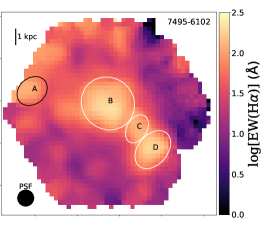
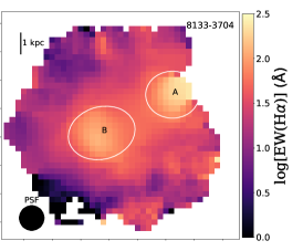
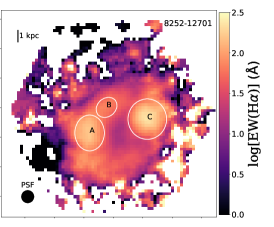
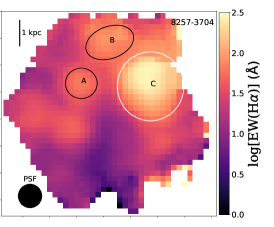
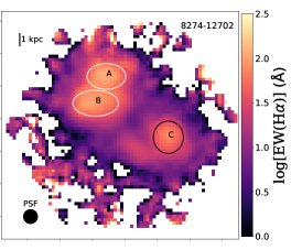
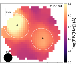
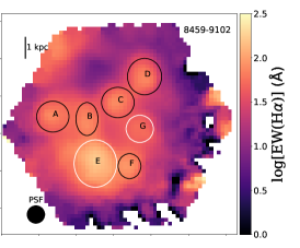
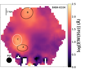
We then carried out two separate analyses on these 12 MaNGA galaxies. The first analysis uses global spectra of each galaxy, only considering spaxels with H$\alpha$ equivalent widths of EW(H$\alpha$) $>30$Å, to minimise contamination from diffuse ionised gas (DIG) emission. The second analysis utilises the IFU capabilities of MaNGA to study distinct regions within these galaxies. We study large H$\alpha$-emitting regions which we term ‘Hii blobs’ because their effective spatial resolution is in the range 0.8 to 1.4 kpc (2.3 to 2.9”), which is several times larger than that of typical Hii regions. We select spaxels with H$\alpha$ equivalent width (EW) of $>50$Å and H$\alpha$ signal-to-noise ratio (S/N) of $>50$, identifying distinct high-EW(H$\alpha$) blobs from the resulting maps by eye (see Appendix B), and then extracting spectra from elliptical regions over each blob.

To be able to accurately measure the nebular emission lines without loss of flux from stellar absorption, we removed the stellar continuum from the total emission spectra by fitting each pixel in the MaNGA data cube with the spectral synthesis code starlight. Subtracting the best-fit stellar component model from the total emission spectrum at each pixel then left us with the gas-only emission spectrum. Emission line fluxes were then measured using Gaussian fits, where in the case of line doublets, the line widths were constrained so that both lines in the doublet had the same velocity width. All fits were checked by eye to verify that the procedure was not fitting a Gaussian to noise. In particular, in the case of weak lines, the best-fit line peak (and thus implied redshift) and line widths were compared to the fits to stronger lines. In those cases where the line was not detected or the best-fit Gaussian was fitting noise, the fit was further constrained by fixing the line width and peak position to the best-fit parameters from fits to stronger lines of the same element. The resulting line fluxes are provided in Table LABEL:tab:MaNGA_HIIblob_data for our Hii blob spectra and Table 2 for our global spectra.

In both analyses, we limit our study to only those systems with S/N($[\textnormal{{Oiii}}]$$\lambda$4363) and S/N($[\textnormal{{Oii}}]$$\lambda\lambda$7320,7330) $\geq 3$. This criterion was applied to ensure that well-constrained $T_{\textnormal{e}}$-based oxygen abundances could be obtained. For our sample of 23 Hii blobs, the mean S/N of the $[\textnormal{{Oiii}}]$$\lambda$4363 line is 6.7, and for the $[\textnormal{{Oii}}]$$\lambda\lambda$7320,7330 doublet is 23.1. All our MaNGA galaxies exhibit strong H$\alpha$ lines, with $F_{\textnormal{obs}}(\textnormal{H}\alpha)\geq 1.0\times{}10^{-15}\,\textnormal{erg}\,\textnormal{s}^{-1}\,\textnormal{cm}^{-2}$.

Our MaNGA sample provides an interesting and relatively new perspective on the low-redshift mass-metallicity relation because all its galaxies lie on or very close to the main sequence of star formation (see §3), whereas most other studies of individual galaxies with $\textnormal{$Z_{\textnormal{Te}}${}}\gtrsim 8.0$ are focused on higher-SFR systems (e.g. Izotov et al. 2006; Hirschauer et al. 2015, 2018).

3 Selection effects

Our combined dataset comprises systems of various different physical sizes, from individual Hii regions (e.g. the Bresolin et al. 2009 sample), to composite ISM regions (e.g. our MaNGA sample), to integrated galaxy spectra (e.g. the Ly et al. 2016a sample). It is also assembled from various different studies, each with different selection criteria. Therefore, it is important that selection effects are assessed.

One concern is that our $T_{\textnormal{e}}$ measurements could be dependent on the physical size of the system. It has been established that the blending of emission from multiple Hii regions of different temperatures within one spectrum can bias estimates of $T_{\textnormal{e}}(\textnormal{{Oii}})$ high when inferring it from $T_{\textnormal{e}}(\textnormal{{Oiii}})$ measurements (Kobulnicky et al., 1999; Pilyugin et al., 2010; Sanders et al., 2017). However, we show in §5.2.4 that our new $T_{\textnormal{e}}(\textnormal{{Oiii}})$-$T_{\textnormal{e}}(\textnormal{{Oii}})$ relation performs equally well for both individual and composite Hii-region spectra, in part because we have included a range of system sizes in our calibration sample.

Similarly, the possible inclusion of systems with contaminated $[\textnormal{{Oii}}]$$\lambda\lambda$7320,7330 auroral lines could affect our results. We have therefore run our analysis on a number of sub-samples, including (a) only systems with high spatial resolution (as described above), (b) only systems with the theoretically expected ratio of the $[\textnormal{{Oii}}]$ auroral line doublet, $r^{\prime}=\textnormal{$[\textnormal{{Oii}}]${}}\lambda 7320/\textnormal{$[\textnormal{{Oii}}]${}}\lambda 7330$, (c) only systems with similar $T_{\textnormal{e}}(\textnormal{{Oii}})$ and $T_{\textnormal{e}}(\textnormal{{Nii}})$ measurements, (d) using the method from Izotov et al. (2006) for obtaining $\textnormal{O}^{+}/\textnormal{H}^{+}$ that does not require $[\textnormal{{Oii}}]$ auroral lines, and (e) discarding $T_{\textnormal{e}}(\textnormal{{Oii}})$ measurements altogether and using $T_{\textnormal{e}}(\textnormal{{Nii}})$ measurements instead. These sub-samples are discussed in §5.2.2 and Appendix A. We find our results hold for all of these sub-samples, indicating that our new calibration of the $T_{\textnormal{e}}(\textnormal{{Oiii}})$ –$T_{\textnormal{e}}(\textnormal{{Oii}})$ relation (see §5.1) is not significantly affected by contamination of key auroral lines.

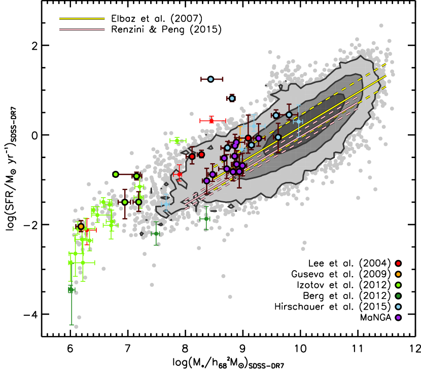
A potential concern for our analysis of the mass-metallicity relation is that datasets such as ours, which require auroral-line detections, can be biased towards starburst galaxies. To assess this, Fig. 1 shows the $M_{*}$-SFR relation for our dataset (coloured points) alongside a typical star-forming sample of 109,678 SDSS-DR7 galaxies below $z=0.3$ from the study of Yates et al. (2012) (grey contours). To facilitate a fair comparison, only the 55 galaxies from our dataset with a counterpart in the SDSS-DR7 spectroscopic catalogue are considered, and their stellar masses and SFRs are taken from the SDSS-DR7 for this plot. While we do have some systems which are highly star-forming for their mass, there are also a significant number of systems that lie within the $1\sigma$ dispersion of the star-forming main sequence of Elbaz et al. (2007) below $\textnormal{log}(M_{*}/\,\textnormal{M}_{\textnormal{\astrosun}})=10.0$ ($\sim{}45$% of our SDSS-matched systems). These galaxies are predominantly from our new MaNGA sample, highlighting its important role in this analysis. We therefore conclude that our dataset is relatively representative of the low-redshift star-forming population.

Figure 1: $M_{*}$-SFR relation for 55 galaxies in our low-redshift dataset with counterparts in the SDSS-DR7 catalogue. Local ‘main sequence’ relations from Elbaz et al. (2007) and Renzini & Peng (2015) are also plotted for comparison, alongside a star-forming galaxy sample from the SDSS-DR7 (grey contours and points, Yates et al. 2012). Points with black outlines represent systems with direct $Z_{\textnormal{Te}}$ estimates, whereas those without represent those with semi-direct $Z_{\textnormal{Te}}$ estimates.

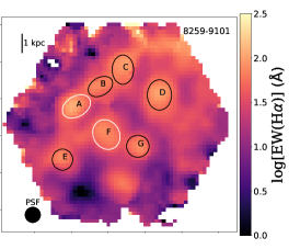
Finally, we also checked that we are not preferentially selecting the lowest-metallicity regions within our MaNGA galaxies by requiring S/N($[\textnormal{{Oiii}}]$$\lambda$4363) $>3.0$. To do this, we measured the metallicity via the $R_{23}$ strong-line diagnostic for every Hii blob within MaNGA systems 8259-9101 and 8459-9102, in order to determine their rough, relative oxygen abundances. Both these systems contain 7 blobs each, allowing a more insightful comparison than for those systems with fewer distinct regions. We use the theoretically-derived $R_{23}$ diagnostic provided by Kewley & Dopita (2002) and an iterative procedure to obtain both the ionisation parameter, $U$, and $Z_{\textnormal{R23}}$ (see Kewley & Dopita 2002, section 6). We find that those Hii blobs which make it into our $T_{\textnormal{e}}$-based sample do not form a special sub-set of the lowest-metallicity regions. In fact, we are able to detect $[\textnormal{{Oiii}}]$$\lambda$4363 in some of the most metal-rich regions in these galaxies.

4 Derived properties

4.1 Stellar masses

The majority of the systems in our dataset have stellar masses taken either from the Sloan Digital Sky Survey MPA-JHU data release 7 (SDSS-DR7, Abazajian et al. 2009) or the NASA-Sloan Atlas v0_1_2 (NSA, Blanton et al. 2011).

Given that stellar masses are presented in units of $h_{68}^{-2}\,\textnormal{M}_{\textnormal{\astrosun}}$ in this work, we have multiplied all SDSS-DR7 masses by the small factor $0.7^{2}/0.68^{2}=1.06$ and all NSA masses by the larger factor $1^{2}/0.68^{2}=2.16$ to maintain consistency throughout.

When stellar masses are available from both catalogues, we adopted those provided by the NSA as they do not suffer from the systematic flux under-estimation for extended systems that SDSS-DR7 stellar masses do, due to improved background subtraction (Blanton et al., 2011). This is particularly important for dwarf galaxies such as those in our study, as these tend to be nearby and therefore more extended on the sky.

The systems with the largest discrepancies in mass estimate between these two catalogues tend to have low specific SFRs ($\textnormal{sSFR}\equiv{}\textnormal{SFR}/M_{*}$). Galaxies with typical or high SFRs for their mass (such as those in our dataset) tend to have discrepancies of less than 1 order of magnitude. We have therefore corrected all SDSS-DR7 stellar masses used in this work, by fitting the $M_{*\textnormal{SDSS-DR7}}$-$M_{*\textnormal{NSA}}$ relation for the 41 galaxies in our low-redshift dataset that are present in both these catalogues with a second-order polynomial given by:

$$\textnormal{log}(M_{*}/h_{68}^{-2}\,\textnormal{M}_{\textnormal{\astrosun}})_{\textnormal{NSA}}=2.81707+0.542641x+0.0181975x^{2}\;\;,$$ (1)

in the range $6.0<x<10.0$, where $x=\textnormal{log}(M_{*}/h_{68}^{-2}\,\textnormal{M}_{\textnormal{\astrosun}})_{\textnormal{SDSS-DR7}}$. This yields a range of correction factors between 1.01 for high-mass systems to 1.12 for low-mass systems.

Masses for the remaining 46 per cent of systems (from NGC300, SLSN hosts, and the Berg et al. 2012 and Ly et al. 2016b samples) are taken directly from the literature.

4.2 Dust corrections

In order to make our dataset as homogeneous as possible, we apply exactly the same reddening corrections to all line fluxes for all systems. For those literature samples where uncorrected line fluxes are not provided, we first re-redden the fluxes by reversing the particular correction used in that work, and then correct all observed fluxes using the following two-step process. Firstly, we correct all lines for Milky Way dust extinction using the Cardelli et al. (1989) extinction law, an extinction factor of $R_{\textnormal{V}}=3.1^{+2.7}_{-1.0}$, and Milky Way reddening along the line of sight from the Schlafly & Finkbeiner (2011) Galactic reddening map. A fit to the wavelength-dependent uncertainty on the extinction law provided by Cardelli et al. (1989), as well as on their measured value of $R_{\textnormal{V}}$, is also folded-in to the error propagation for our dust corrections.

Secondly, we correct for internal attenuation within the host system using the Calzetti et al. (2000) attenuation law for star-forming galaxies, $k^{\prime}(\lambda,R^{\prime}_{\textnormal{V}})$, and

$$F_{\textnormal{cor}}(\lambda)=F_{\textnormal{obs}}(\lambda)\,10^{0.176\,E(B-V)_{\textnormal{gas}}\,k^{\prime}(\lambda,R^{\prime}_{\textnormal{V}})}\;\;,$$ (2)

where $R^{\prime}_{\textnormal{V}}=4.05\textnormal{\scriptsize{$\pm 0.80$}}$, and $E(B-V)_{\textnormal{gas}}$ is the colour excess of the ionised gas (see Calzetti 1997). An intrinsic Balmer decrement of 2.86 is assumed, which is suitable for case B recombination in local star-forming galaxies with $N_{\textnormal{e}}\sim{}100\,\textnormal{cm}^{3}$ and $T_{\textnormal{e}}\sim{}10000$ K (Osterbrock, 1989).

We note that this method always returns a non-zero correction to the observed fluxes, even when the internal extinction is determined to be zero, due to the ever-present Milky Way extinction to the redshifted line. Applying uniform dust reddening corrections in this way decreases slightly the scatter in the final electron temperature and oxygen abundance distributions.

4.3 Electron temperatures and oxygen abundances

In order to calculate electron temperatures ($T_{\textnormal{e}}$) and $T_{\textnormal{e}}$-based metallicities ($Z_{\textnormal{Te}}$) for our dataset, we adopt the formalism developed by Nicholls et al. (2013, 2014b, 2014a). Those works utilised the MAPPINGS IV photoionisation code (Dopita et al., 2013) to fit relations between collisionally excited line (CEL) flux ratios from observed spectra to key physical properties of the gas. These relations allow a dependence on the electron density and electron energy distribution, and incorporate updated atomic data, including revised collision strengths for many ionic species. The atomic datasets used in MAPPINGS IV are listed in table 1 of Nicholls et al. (2013). The collision strengths for the key oxygen ions used in this work are taken from Tayal (2007) for $\textnormal{O}^{+}$, and from Aggarwal (1993); Lennon & Burke (1994); Aggarwal & Keenan (1999); and Palay et al. (2012) for $\textnormal{O}^{++}$ (with those for the ${}^{1}D_{2}$ and ${}^{1}S_{0}$ levels from which the $\lambda\lambda$4959,5007 and $\lambda$4363 lines originate taken from Palay et al. 2012).

The absolute accuracy of collision strength and transition probability estimates is very difficult to constrain, due to the complex calculations and assumptions involved in their determination. Therefore, we have included an additional error on all the electron densities, electron temperatures, and ionic abundances we calculate in this work, to account for the uncertainty in atomic data. This could be particularly important for our $T_{\textnormal{e}}(\textnormal{{Oiii}})$ and $\textnormal{O}^{++}/\textnormal{H}^{+}$ estimates, as the $\textnormal{O}^{++}$ collision strengths provided by Palay et al. 2012 are known to return electron temperatures for Hii regions that are up to $\sim{}600$ K lower than other Breit-Pauli R-matrix based methods from the literature (see Storey et al. 2014; Izotov et al. 2015; Tayal & Zatsarinny 2017).

We account for such atomic data discrepancies by adopting the typical uncertainties found for Hii regions with $N_{\textnormal{e}}<1000\ \textnormal{cm}^{-3}$ by Juan de Dios & Rodríguez (2017) when comparing 52 different atomic datasets from the literature, including that of Palay et al. (2012). This leads to the following additional errors, which are propagated through all the calculations we make hereafter: $\sigma(N_{\textnormal{e}})=0.16$ dex, $\sigma[\textnormal{$T_{\textnormal{e}}(\textnormal{{Nii}})${}}]=0.02$ dex, $\sigma[\textnormal{$T_{\textnormal{e}}(\textnormal{{Oii}})${}}]=0.02$ dex, $\sigma[\textnormal{$T_{\textnormal{e}}(\textnormal{{Oiii}})${}}]=0.025$ dex, $\sigma[\textnormal{$\textnormal{O}^{+}/\textnormal{H}^{+}${}}]=0.1$ dex, $\sigma[\textnormal{$\textnormal{O}^{++}/\textnormal{H}^{+}${}}]=0.075$ dex. These additional uncertainties increase the typical error on our $Z_{\textnormal{Te}}$ estimates by 0.035 dex.

In this work, we assume thermal equilibrium in the gas (i.e. a Maxwell-Boltzmann electron energy distribution), adopting the following expression for the electron temperature in Kelvin;

$$T_{\textnormal{e}}=a\left[-\textnormal{log}\left(\frac{R_{\textnormal{obs}}}{1+d\left(N_{\textnormal{e}}/T^{1/2}_{\textnormal{e}}\right)}\right)-b\;\right]^{-c}\;\;,$$ (3)

where $R_{\textnormal{obs}}$ is the reddening-corrected flux ratio of the particular ionic species, and $N_{\textnormal{e}}$ is the electron density in cm^-3. The values of the coefficients $a$, $b$, $c$, and $d$ are also dependent on the ionic species and electron density, and have been calculated by Nicholls et al. (2013, their tables 4 and 5) by fitting to the output from the MAPPINGS IV code. The flux ratios we consider in this work for $R_{\textnormal{obs}}$ are:

$$R({\textsc{Oii}}) =\textnormal{$[\textnormal{{Oii}}]$}\lambda\lambda 7320,7330\;/\;\textnormal{$[\textnormal{{Oii}}]$}\lambda\lambda 3726,3729\;\;,$$

$$R({\textsc{Oiii}}) =\textnormal{$[\textnormal{{Oiii}}]$}\lambda 4363\;/\;\textnormal{$[\textnormal{{Oiii}}]$}\lambda\lambda 4959,5007\;\;,$$

$$R({\textsc{Nii}}) =\textnormal{$[\textnormal{{Nii}}]$}\lambda 5755\;/\;\textnormal{$[\textnormal{{Nii}}]$}\lambda 6584\;\;,$$ (4)

where the nitrogen ratio, $R(\textsc{Nii}){}$, is only used for a subset of systems for which the particularly weak $[\textnormal{{Nii}}]$$\lambda 5755$ auroral line was detected (see Appendix A). We then solve Eq. 3 iteratively to obtain $T_{\textnormal{e}}$. Convergence is typically achieved within three iterations for $T_{\textnormal{e}}(\textnormal{{Oiii}})$, and five iterations for $T_{\textnormal{e}}(\textnormal{{Oii}})$.

We checked that the electron temperatures obtained from this procedure are very similar to those obtained by numerically solving the complete statistical equilibrium equations using the latest version of the pyneb package (Luridiana et al., 2013), which is a revised version of the nebular/temden routines provided by IRAF (Shaw & Dufour, 1995). When assuming the same atomic data, we find the median difference in direct $T_{\textnormal{e}}(\textnormal{{Oiii}})$ is only $\sim{}40$ K for our dataset, and the median difference in direct $T_{\textnormal{e}}(\textnormal{{Oii}})$ is only 132 K. This indicates that analytic expressions such as Eq. 3 above (or eq. 5.4 from Osterbrock & Ferland 2006) are valid in the temperature and density regime studied here.

We did not make any additional corrections to flux ratios to account for Eddington bias (Eddington, 1913) in this work, as these are believed to be negligible and depend sensitively on the instrument and type of observation made. However, we note that when applying the corrections to $R(\textsc{Oiii})$ provided by Ly et al. (2016a) from their MMT and Keck data, the mean $Z_{\textnormal{Te}}$ for our sample increases by only 0.026 dex, due to the reduction in the assumed $[\textnormal{{Oiii}}]$$\lambda 4363$ line strength for systems with S/N($[\textnormal{{Oiii}}]$$\lambda 4363$) $\lesssim{}7$.

An estimate of $N_{\textnormal{e}}$ is obtained from the ratio of [Sii] lines, as provided by O’Dell et al. (2013) based on the work of Osterbrock & Ferland (2006);

$$\textnormal{log}(N_{\textnormal{e}}/\textnormal{cm}^{-3})=4.705-\left(1.9875\;\frac{\textnormal{[S{ii}]}\lambda 6716}{\textnormal{[S{ii}]}\lambda 6731}\right)\;\;.$$ (5)

Although $T_{\textnormal{e}}(\textnormal{{Oiii}})$ exhibits a negligible dependence on the electron density for the typical range of $N_{\textnormal{e}}$ observed in local Hii regions, the MAPPINGS IV code does infer an important effect for $T_{\textnormal{e}}(\textnormal{{Oii}})$, such that electron densities above $100\;\textnormal{cm}^{-3}$ would lead to an over-estimate in $T_{\textnormal{e}}(\textnormal{{Oii}})$ by up to 2000 K if not accounted for.

Following Nicholls et al. (2014b), and making the common assumption of a constant collision strength and a uniform electron temperature in each ionic zone, we then obtain singly- and doubly-ionised oxygen abundances as follows:

$$\textnormal{$\textnormal{O}^{+}/\textnormal{H}^{+}$}\;= \;\frac{\textnormal{$[\textnormal{{Oii}}]$}\lambda\lambda 3726,3729}{\textnormal{H}_{\beta}}\;g_{1}\;\alpha_{\textnormal{H$\beta$}}\;\sqrt{\textnormal{$T_{\textnormal{e}}(\textnormal{{Oii}})$}}$$

$$\cdot\textnormal{exp}\left[E_{12}/k\textnormal{$T_{\textnormal{e}}(\textnormal{{Oii}})$}\right]\;\times\;\frac{\beta}{E_{12}\Upsilon_{12}}$$ (6)

$$\textnormal{$\textnormal{O}^{++}/\textnormal{H}^{+}$}\;= \;\frac{\textnormal{$[\textnormal{{Oiii}}]$}\lambda\lambda 4959,5007}{\textnormal{H}_{\beta}}\;g_{1}\;\alpha_{\textnormal{H$\beta$}}\;\sqrt{\textnormal{$T_{\textnormal{e}}(\textnormal{{Oiii}})$}}$$

$$\cdot\textnormal{exp}\left[E_{12}/k\textnormal{$T_{\textnormal{e}}(\textnormal{{Oiii}})$}\right]\;\times\;\frac{\beta}{E_{12}\Upsilon_{12}}\;\;,$$ (7)

where $g_{1}$ is the statistical weight of the ground state ($g_{1}=4$ for $\textnormal{O}^{+}$ and 9 for $\textnormal{O}^{++}$), $\alpha_{\textnormal{H$\beta$}}$ is the $T_{\textnormal{e}}(\textnormal{{Oiii}})$-dependent effective emissivity for H_β assuming Case B recombination, $E_{12}=hc/\lambda_{\textnormal{avg}}$ is the energy difference between the collisionally-excited state and the ground state (where $\lambda_{\textnormal{{OII{}}}}=3727$ Å and $\lambda_{\textnormal{{OIII{}}}}=4997$ Å are the flux-weighted average wavelengths for the $[\textnormal{{Oii}}]$ and $[\textnormal{{Oiii}}]$ lines considered here), $k$ is Boltzmann’s constant, $\Upsilon_{12}$ is the temperature-dependent net effective collision strength for the transition in question, $\beta=(h^{4}/8\pi^{3}m_{\textnormal{e}}^{3}k)^{-1/2}=115885.4\;\textnormal{K}^{-1/2}\,\textnormal{cm}^{-3}\,\textnormal{s}$ is the constant factor from the collision rate coefficient, $h$ is Planck’s constant, and $m_{\textnormal{e}}$ is the mass of an electron. We refer the reader to Nicholls et al. (2014a, section 4.1) for more details, including the equations used to determine $\alpha_{\textnormal{H$\beta$}}$ and $\Upsilon_{12}$.

An estimate of the total oxygen abundance, $Z_{\textnormal{Te}}$, can then be obtained by summing the abundances of these two ionic species;

$$\textnormal{$Z_{\textnormal{Te}}$}\equiv 12+\textnormal{log}(\textnormal{$\textnormal{O}^{+}/\textnormal{H}^{+}$}+\textnormal{$\textnormal{O}^{++}/\textnormal{H}^{+}$})\;\;,$$ (8)

assuming that higher and lower ionised states of oxygen have a negligible contribution (e.g. Stasińska et al. 2012). We note here that this simple addition of the two measured oxygen abundances assumes that either the $\textnormal{O}^{+}$ and $\textnormal{O}^{++}$ zones are co-spatial, or the amount of H⁺ in each zone is the same.

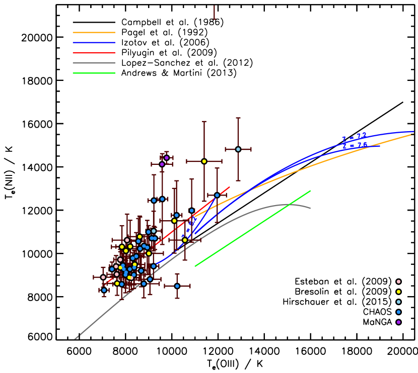
For many systems, the weak $[\textnormal{{Oii}}]$$\lambda\lambda 7320,7330$ line doublet is either not detected or is redward of the wavelength range of the spectrograph used. In such cases, a direct measurement of the $[\textnormal{{Oii}}]$ temperature is not possible using Eq. 3, and one must instead rely upon either an alternative ionic temperature (see Appendix A) or an approximation inferred from the measured $[\textnormal{{Oiii}}]$ temperature (e.g. Campbell et al. 1986; Garnett 1992; Pagel et al. 1992; Izotov et al. 2006; Pilyugin 2007; Pilyugin et al. 2009; López-Sánchez et al. 2012; Andrews & Martini 2013; Nicholls et al. 2014b). Such $T_{\textnormal{e}}(\textnormal{{Oiii}})$ – $T_{\textnormal{e}}(\textnormal{{Oii}})$ relations are discussed in the following section.

5 The $\boldsymbol{\textnormal{$T_{\textnormal{e}}(\textnormal{{Oiii}})${}}-\textnormal{$T_{\textnormal{e}}(\textnormal{{Oii}})${}}}$ relation

Fig. 2 shows $T_{\textnormal{e}}(\textnormal{{Oiii}})$ versus $T_{\textnormal{e}}(\textnormal{{Oii}})$ for our 130 direct-$Z_{\textnormal{Te}}$ systems. Each system is coloured to indicate the base sample to which it belongs. Six empirically- or theoretically-derived $T_{\textnormal{e}}(\textnormal{{Oiii}})$ – $T_{\textnormal{e}}(\textnormal{{Oii}})$ relations from the literature are also plotted for comparison.

The mean S/N of the auroral lines used here are S/N$(\textnormal{$[\textnormal{{Oiii}}]$}\lambda{}4363)=18.2$ and S/N$(\textnormal{$[\textnormal{{Oii}}]$}\lambda{}\lambda{}7320,7330)=22.5$. The S/N of the nitrogen auroral line for the 53 systems with reported detections is S/N$(\textnormal{$[\textnormal{{Nii}}]$}\lambda{}5755)=8.2$ (see Appendix A).

Figure 2: $T_{\textnormal{e}}(\textnormal{{Oiii}})$-$T_{\textnormal{e}}(\textnormal{{Oii}})$ plane containing our 130 systems with direct $Z_{\textnormal{Te}}$ estimates [i.e. those for which both $T_{\textnormal{e}}(\textnormal{{Oiii}})$ and $T_{\textnormal{e}}(\textnormal{{Oii}})$ can be calculated from auroral lines]. Six empirically- or theoretically-derived $T_{\textnormal{e}}(\textnormal{{Oiii}})$ – $T_{\textnormal{e}}(\textnormal{{Oii}})$ relations from Campbell et al. (1986, black), Pagel et al. (1992, orange), Izotov et al. (2006, blue, for metallicities of 7.2, 7.6, and 8.2), Pilyugin et al. (2009, red), López-Sánchez et al. (2012, grey), and Andrews & Martini (2013, green, as defined in Ly et al. 2016a), are also plotted for comparison. Our dataset reveals a much broader distribution of $T_{\textnormal{e}}(\textnormal{{Oii}})$/$T_{\textnormal{e}}(\textnormal{{Oiii}})$ ratios than is expected from the literature relations.

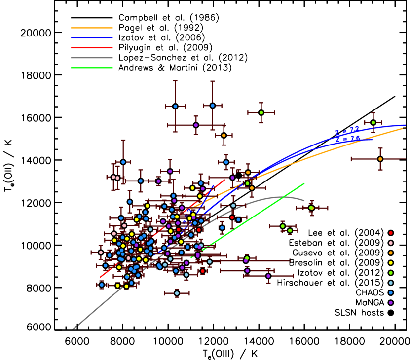
We first note that the distribution of our dataset across the $T_{\textnormal{e}}(\textnormal{{Oiii}})$ – $T_{\textnormal{e}}(\textnormal{{Oii}})$ parameter space is quite broad, including a significant fraction of systems exhibiting lower $T_{\textnormal{e}}(\textnormal{{Oii}})$ than $T_{\textnormal{e}}(\textnormal{{Oiii}})$ (see also Kennicutt et al. 2003). Consequently, there appears to be no clear one-to-one correlation between $T_{\textnormal{e}}(\textnormal{{Oiii}})$ and $T_{\textnormal{e}}(\textnormal{{Oii}})$ in Fig. 2, indicating that none of the common $T_{\textnormal{e}}(\textnormal{{Oiii}})$ – $T_{\textnormal{e}}(\textnormal{{Oii}})$ relations plotted is particularly representative of the true range of $T_{\textnormal{e}}(\textnormal{{Oii}})$/$T_{\textnormal{e}}(\textnormal{{Oiii}})$ ratios in this dataset. A similar conclusion can be drawn from the samples considered by Izotov et al. (2006, fig. 4a) and Andrews & Martini (2013, fig. 3), and is also discussed by Yan (2018) in reference to their Cloudy 17.00 (Ferland et al., 2017) modelling.

Motivated by this issue, in the following sections we develop a new empirical $T_{\textnormal{e}}(\textnormal{{Oiii}})$ - $T_{\textnormal{e}}(\textnormal{{Oii}})$ relation, which allows for a broader range of $T_{\textnormal{e}}(\textnormal{{Oii}})$/$T_{\textnormal{e}}(\textnormal{{Oiii}})$ ratios.

Figure 3: Schematic diagram qualitatively illustrating the expected relation between $T_{\textnormal{e}}(\textnormal{{Oiii}})$ and $T_{\textnormal{e}}(\textnormal{{Oii}})$ at fixed $Z_{\textnormal{Te}}$ in different regions of the $T_{\textnormal{e}}(\textnormal{{Oiii}})$ – $T_{\textnormal{e}}(\textnormal{{Oii}})$ plane. Grey lines illustrate arbitrary tracks of constant $Z_{\textnormal{Te}}$. Regions A and B denote the approximate regimes where $Z_{\textnormal{Te}}$ is likely dominated by only one ionisation state of oxygen ($\textnormal{O}^{++}/\textnormal{H}^{+}$ or $\textnormal{O}^{+}/\textnormal{H}^{+}$, respectively). Region C denotes the approximate regime where both ionisation states are likely significant, and a uniform anti-correlation between $T_{\textnormal{e}}(\textnormal{{Oiii}})$ and $T_{\textnormal{e}}(\textnormal{{Oii}})$ at fixed $Z_{\textnormal{Te}}$ is expected. We stress that the simplified picture illustrated here may change if, for example, the nebulae are not radiation bounded, or if the density distribution in the $\textnormal{O}^{++}$ and $\textnormal{O}^{+}$ zones are very different.

5.1 A new empirical $T_{\textnormal{e}}(\textnormal{{Oiii}})$ – $T_{\textnormal{e}}(\textnormal{{Oii}})$ relation

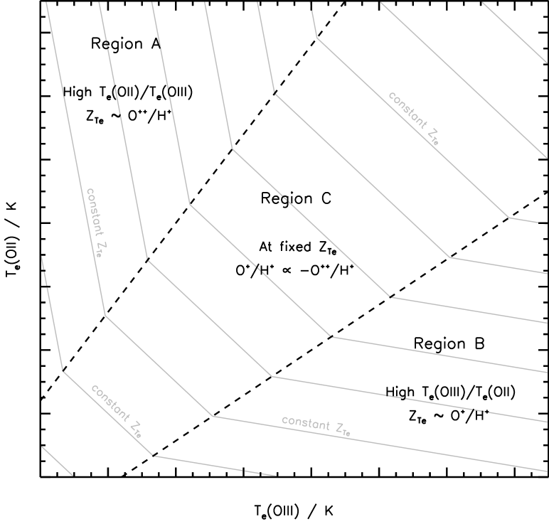
The form of our new $T_{\textnormal{e}}(\textnormal{{Oiii}})$ – $T_{\textnormal{e}}(\textnormal{{Oii}})$ relation is motivated by two important considerations. First, that electron temperature and oxygen abundance are anti-correlated. Consequently, we would expect systems with $T_{\textnormal{e}}(\textnormal{{Oiii}})$ $<$ $T_{\textnormal{e}}(\textnormal{{Oii}})$ to have $\textnormal{O}^{++}/\textnormal{H}^{+}$ $>$ $\textnormal{O}^{+}/\textnormal{H}^{+}$, and for their total $Z_{\textnormal{Te}}$ to be relatively insensitive to $T_{\textnormal{e}}(\textnormal{{Oii}})$. This is illustrated by Region A in the schematic in Fig. 3. Likewise, we would expect systems with $T_{\textnormal{e}}(\textnormal{{Oiii}})$ $>$ $T_{\textnormal{e}}(\textnormal{{Oii}})$ to have $\textnormal{O}^{++}/\textnormal{H}^{+}$ $<$ $\textnormal{O}^{+}/\textnormal{H}^{+}$, and therefore their total $Z_{\textnormal{Te}}$ to be relatively insensitive to $T_{\textnormal{e}}(\textnormal{{Oiii}})$ (see Region B in Fig. 3). Second, that there is an empirical anti-correlation between $T_{\textnormal{e}}(\textnormal{{Oiii}})$ and $T_{\textnormal{e}}(\textnormal{{Oii}})$ at fixed $Z_{\textnormal{Te}}$ for our dataset, (see coloured points in Fig. 5 below). This is also expected theoretically from the equations laid-out in §4.3, as $\textnormal{$\textnormal{O}^{+}/\textnormal{H}^{+}${}}\propto-\textnormal{$\textnormal{O}^{++}/\textnormal{H}^{+}${}}$ at fixed $Z_{\textnormal{Te}}$. This is in contrast to what is typically assumed for other metallicity-dependent $T_{\textnormal{e}}(\textnormal{{Oiii}})$ – $T_{\textnormal{e}}(\textnormal{{Oii}})$ relations in the literature (e.g. Izotov et al. 2006; Nicholls et al. 2014b). The anti-correlation we find is illustrated by Region C in Fig. 3 by grey lines of constant $Z_{\textnormal{Te}}$.

Figure 4: Top panel: Relation between $Z_{\textnormal{Te}}$ and the hyperbolic semi-axis $a$ for our direct dataset. Linear fits to the data (Eq. 5.1) are shown for our Bayesian analysis (dark grey solid line) and least squares fitting (black solid line). Dashed lines indicate the 1$\sigma$ scatter around the distribution of $Z_{\textnormal{Te}}$ values for the least-squares fit. The grey area around the Bayesian best-fit indicates the range of possible fits considering the full covariance matrix. Bottom panels: $Z_{\textnormal{Te}}$-$T_{\textnormal{e}}(\textnormal{{Oiii}})$ and $Z_{\textnormal{Te}}$-$T_{\textnormal{e}}(\textnormal{{Oii}})$ relations for the same dataset. The large spread in the $Z_{\textnormal{Te}}$-$T_{\textnormal{e}}(\textnormal{{Oii}})$ relation leads to quite discrepant fits being returned by our two statistical fitting methods.

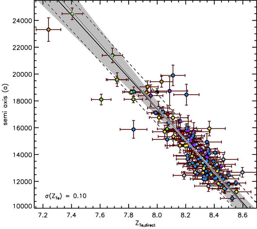
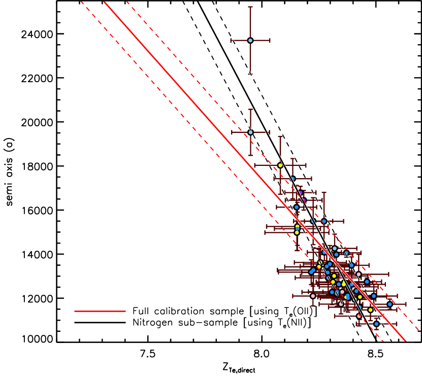
Therefore, we propose a functional form for our new $Z_{\textnormal{Te}}$-dependent $T_{\textnormal{e}}(\textnormal{{Oiii}})$ – $T_{\textnormal{e}}(\textnormal{{Oii}})$ relation which broadly embodies these two considerations, and allows for an unrestricted range of possible $T_{\textnormal{e}}(\textnormal{{Oii}})$/$T_{\textnormal{e}}(\textnormal{{Oiii}})$ ratios. To do this, we adopt the equation of a rectangular hyperbola, centered on 0 Kelvin, given by

$$\textnormal{$T_{\textnormal{e}}(\textnormal{{Oii}})$}=\frac{a(\textnormal{$Z_{\textnormal{Te}}${}})^{2}}{2}\,\frac{1}{\textnormal{$T_{\textnormal{e}}(\textnormal{{Oiii}})$}}\;\;,$$ (9)

where $a$ is the hyperbolic semi axis. We then fit $a$ to the directly-measured $Z_{\textnormal{Te}}$ values from our dataset, finding the following linear dependence (see Appendix D for details on our fitting methods):

$$a= -11657.85\textnormal{\scriptsize{$\pm 434.08$}}\;\textnormal{$Z_{\textnormal{Te}}${}}+110655.66\textnormal{\scriptsize{$\pm 3567.40$}} \textnormal{\footnotesize{(Least squares)}}\;,$$

$$a= -12030.22\textnormal{\scriptsize{$\pm 499.37$}}\;\textnormal{$Z_{\textnormal{Te}}${}}+113720.75\textnormal{\scriptsize{$\pm 562.50$}} \textnormal{\footnotesize{(Bayesian)}}\;.$$ (10)

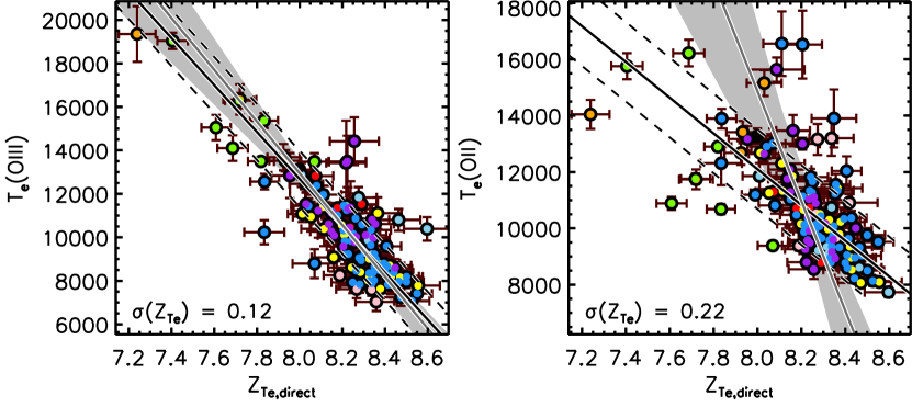
We find that $Z_{\textnormal{Te}}$ is more tightly correlated with $a$ than with $T_{\textnormal{e}}(\textnormal{{Oiii}})$ or $T_{\textnormal{e}}(\textnormal{{Oii}})$ alone. This is illustrated in Fig. 4, which shows the $Z_{\textnormal{Te}}$ – $a$ relation for our direct dataset in the top panel, and the $Z_{\textnormal{Te}}$ – $T_{\textnormal{e}}(\textnormal{{Oiii}})$ and $Z_{\textnormal{Te}}$– $T_{\textnormal{e}}(\textnormal{{Oii}})$ relations in the bottom panels. The standard deviation from least-squares fitting is slightly lower for the $Z_{\textnormal{Te}}$ – $a$ relation [with $\sigma(\textnormal{$Z_{\textnormal{Te}}${}})=0.10$, 0.12, and 0.22, respectively], and that this relation is marginally favoured over the $T_{\textnormal{e}}(\textnormal{{Oiii}})$ or $T_{\textnormal{e}}(\textnormal{{Oii}})$ relations by our Bayesian analysis, with comparative Bayes factors of 1.2 and 2.3, respectively.

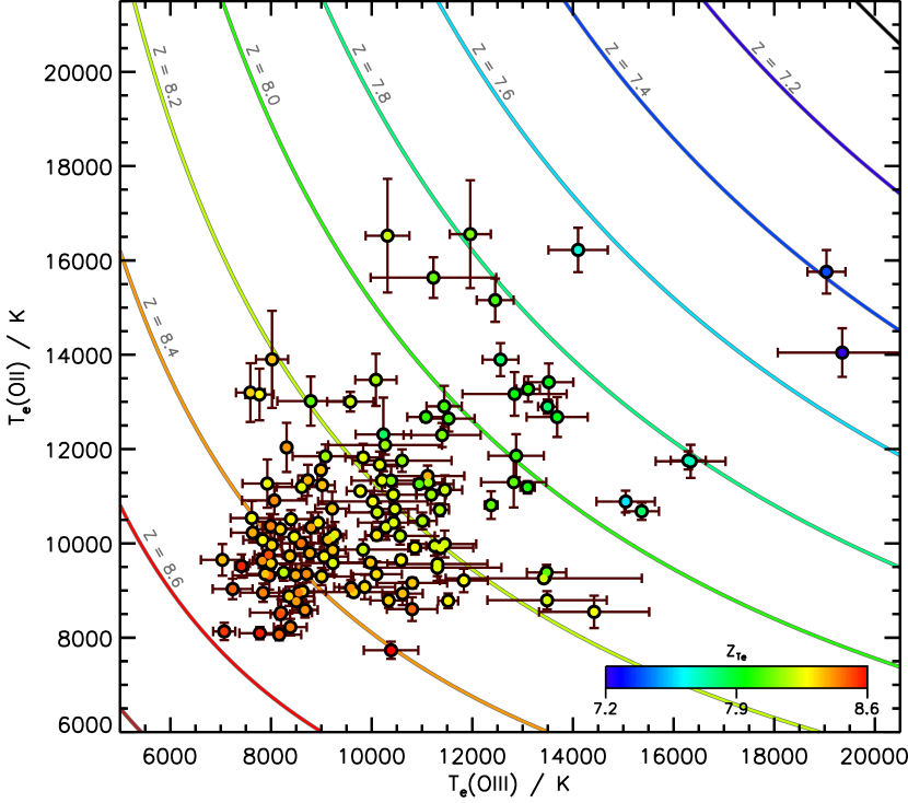
Eq. 9 is plotted for discrete values of $Z_{\textnormal{Te}}$ in Fig. 5, alongside our direct $Z_{\textnormal{Te}}$ systems which are coloured by their direct $Z_{\textnormal{Te}}$. The correspondence between our new relation and the measured $Z_{\textnormal{Te}}$ for our dataset is good across the whole $T_{\textnormal{e}}(\textnormal{{Oiii}})$ – $T_{\textnormal{e}}(\textnormal{{Oii}})$ plane. Eq. 9 can then be solved for both $Z_{\textnormal{Te}}$ and $T_{\textnormal{e}}(\textnormal{{Oii}})$ using fixed-point iteration, similar to the approaches used by Izotov et al. (2006), Pilyugin (2007), and Nicholls et al. (2014b), except that we are explicitly accounting for the interdependence of $Z_{\textnormal{Te}}$ and electron temperature here.

Eqs. 9 and 5.1 can be combined to provide the following equivalent expression for $Z_{\textnormal{Te}}$,

$$\textnormal{$Z_{\textnormal{Te}}${}}= \ 9.49\textnormal{\scriptsize{$\pm 0.05$}}-\frac{\left[2\,\textnormal{$T_{\textnormal{e}}(\textnormal{{Oiii}})${}}\cdot{}\textnormal{$T_{\textnormal{e}}(\textnormal{{Oii}})${}}\right]^{1/2}}{11657.85\textnormal{\scriptsize{$\pm 434.08$}}} \textnormal{\footnotesize{(Least squares)}}\;,$$

$$\textnormal{$Z_{\textnormal{Te}}${}}= \ 9.45\textnormal{\scriptsize{$\pm 0.04$}}-\frac{\left[2\,\textnormal{$T_{\textnormal{e}}(\textnormal{{Oiii}})${}}\cdot{}\textnormal{$T_{\textnormal{e}}(\textnormal{{Oii}})${}}\right]^{1/2}}{12030.22\textnormal{\scriptsize{$\pm 499.37$}}} \textnormal{\footnotesize{(Bayesian)}}\;.$$ (11)

An alternative fit to the $Z_{\textnormal{Te}}$ – $a$ relation, when using $T_{\textnormal{e}}(\textnormal{{Nii}})$ rather than $T_{\textnormal{e}}(\textnormal{{Oii}})$ to determine $\textnormal{O}^{+}$, is discussed in Appendix A.

Figure 5: $T_{\textnormal{e}}(\textnormal{{Oiii}})$-$T_{\textnormal{e}}(\textnormal{{Oii}})$ plane containing our 130 systems with direct $Z_{\textnormal{Te}}$ estimates, as shown in Fig. 2. Here, each system is coloured by its direct $Z_{\textnormal{Te}}$. Our new empirically-derived $T_{\textnormal{e}}(\textnormal{{Oiii}})$ – $T_{\textnormal{e}}(\textnormal{{Oii}})$ relation (Eq. 9) is plotted for discrete values of $Z_{\textnormal{Te}}$ for comparison. There is a good correspondence seen between the metallicites of the data and the relation across this plane.

5.2 A semi-direct abundance deficit at low $\textnormal{O}^{++}$/$\textnormal{O}^{+}$

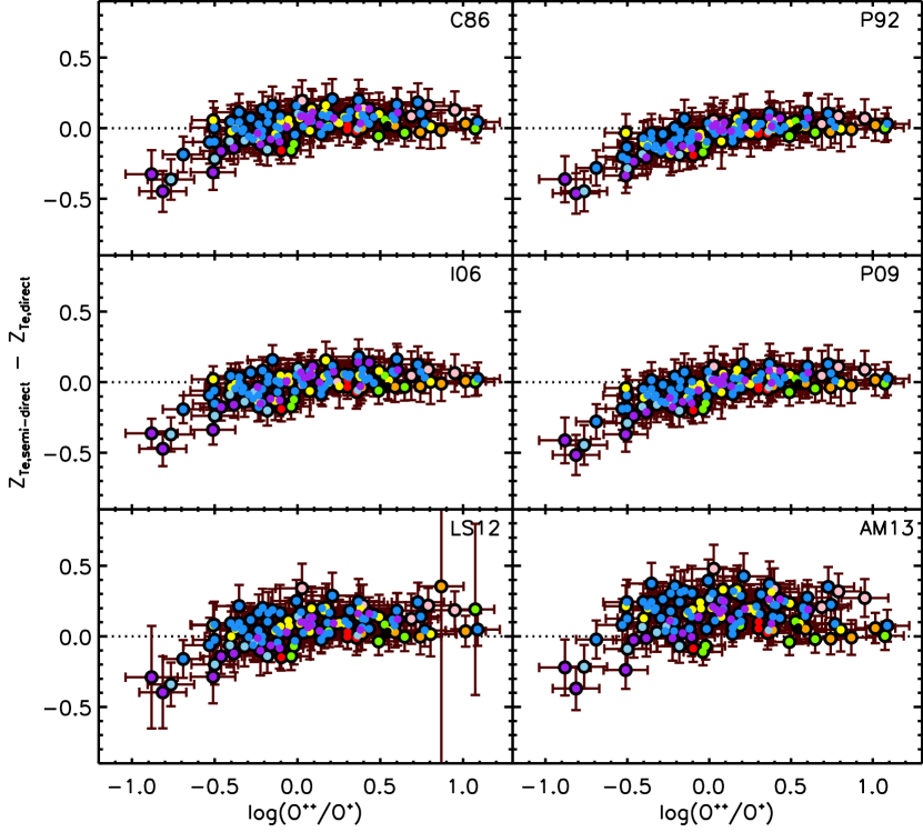
First, we compare the direct and semi-direct $Z_{\textnormal{Te}}$ estimates for our dataset, using each of the six literature $T_{\textnormal{e}}(\textnormal{{Oiii}})$ – $T_{\textnormal{e}}(\textnormal{{Oii}})$ relations considered here. Significantly, we find that all the literature relations under-estimate $Z_{\textnormal{Te}}$ by up to 0.6 dex for low-ionisation systems. This is illustrated in Fig. 6, where the difference between the semi-direct and direct $Z_{\textnormal{Te}}$ estimates is plotted against $\textnormal{O}^{++}$/$\textnormal{O}^{+}$. We hereafter refer to this $Z_{\textnormal{Te}}$ under-estimation as the ‘semi-direct $Z_{\textnormal{Te}}$ deficit’.

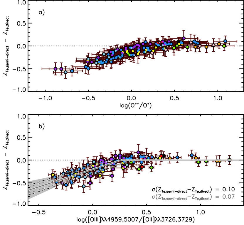
This deficit at low $\textnormal{O}^{++}$/$\textnormal{O}^{+}$ is also present for our new $T_{\textnormal{e}}(\textnormal{{Oiii}})$ –$T_{\textnormal{e}}(\textnormal{{Oii}})$ relation, as shown in panel (a) of Fig. 7. The apparent ubiquity of the semi-direct $Z_{\textnormal{Te}}$ deficit suggests that it is an intrinsic issue for all semi-direct methods that rely on only $T_{\textnormal{e}}(\textnormal{{Oiii}})$ measurements. We have also checked this analysis by using the equations provided by Izotov et al. (2006) to calculate $T_{\textnormal{e}}(\textnormal{{Oiii}})$, $\textnormal{O}^{+}/\textnormal{H}^{+}$, and $\textnormal{O}^{++}/\textnormal{H}^{+}$ (their eqs. 1 to 5) rather than Eqs. 3, 4.3, and 4.3 above, and find that our results are unchanged.

Physically speaking, systems with low $\textnormal{O}^{++}$/$\textnormal{O}^{+}$ ostensibly have a larger $\textnormal{O}^{+}/\textnormal{H}^{+}$ abundance than $\textnormal{O}^{++}/\textnormal{H}^{+}$ abundance, meaning that singly-ionised oxygen dominates their total oxygen budget. Andrews & Martini (2013) have also determined that a significant fraction of higher-mass galaxies appear to have their overall $Z_{\textnormal{Te}}$ dominated by $\textnormal{O}^{+}/\textnormal{H}^{+}$. They find that log($\textnormal{O}^{++}$/$\textnormal{O}^{+}$) typically drops below 0.0 at masses above $\textnormal{log(}M_{*}/\,\textnormal{M}_{\textnormal{\astrosun}})\sim{}8.2$ for stacks of SDSS-DR7 galaxies (their fig. 5c). Similarly, Curti et al. (2017) found that higher-metallicity galaxies have log($\textnormal{O}^{++}$/$\textnormal{O}^{+}$) below 0.0. In what follows, we discuss various possible explanations for the semi-direct $Z_{\textnormal{Te}}$ deficit at low $\textnormal{O}^{++}$/$\textnormal{O}^{+}$ that we find.

Figure 6: Semi-direct $Z_{\textnormal{Te}}$ deficit as a function of $\textnormal{O}^{++}$/$\textnormal{O}^{+}$ when semi-direct $Z_{\textnormal{Te}}$ is calculated using each of the six literature $T_{\textnormal{e}}(\textnormal{{Oiii}})$-$T_{\textnormal{e}}(\textnormal{{Oii}})$ relations considered in this work. Labels in each panel denote which $T_{\textnormal{e}}(\textnormal{{Oiii}})$ – $T_{\textnormal{e}}(\textnormal{{Oii}})$ relation is considered. A similar (although often weaker) anti-correlation is also seen for these literature relations.

5.2.1 Weak auroral lines

Systematic effects on $T_{\textnormal{e}}(\textnormal{{Oiii}})$ due to inaccurate $[\textnormal{{Oiii}}]$$\lambda 4363$ measurements are unlikely to play a significant role as we only consider spectra with S/N($[\textnormal{{Oiii}}]$$\lambda 4363$) $\geq 3.0$. Similarly, a systematic over-estimation of $[\textnormal{{Oii}}]$$\lambda 7320,7330$ fluxes due to poor line fitting is unlikely, as we have also enforced a S/N lower limit of 3.0 for these lines and find an average S/N($[\textnormal{{Oii}}]$$\lambda 7320,7330$) of 22.5. There is also no trend present between S/N($[\textnormal{{Oii}}]$$\lambda\lambda 7320,7330$) and the measured semi-direct $Z_{\textnormal{Te}}$ deficit.

5.2.2 $[\textnormal{{Oii}}]$ line contamination

The $[\textnormal{{Oii}}]$$\lambda\lambda 7320,7330$ auroral line quadruplet lies in a region of the optical spectrum which is populated by a large number of skylines. Additionally, collisional de-excitation, reddening effects, the telluric emission of OH bands, absorption of water bands, and absorption features in the underlying stellar continuum can affect their flux measurements (see e.g. Kennicutt et al. 2003; Pilyugin et al. 2009; Croxall et al. 2015).

When considering our own dataset, we note that collisional de-excitation is already accounted for in the Nicholls et al. (2013) photoionisation models, via an explicit dependence of $T_{\textnormal{e}}$ on electron density. This means that the $T_{\textnormal{e}}(\textnormal{{Oii}})$ and $T_{\textnormal{e}}(\textnormal{{Nii}})$ temperatures we derive for each system are actually quite similar for most of our dataset, as shown in Fig. 15. We have also been particularly careful to accurately and consistently correct all emission line fluxes for reddening (see §4.2), and our MaNGA spectra have been corrected for stellar absorption (see §2). Also, the majority of our dataset lies at redshifts above $z\sim{}0.006$, meaning the $[\textnormal{{Oii}}]$ auroral lines are redshifted away from strong potential contamination from the OH Meinel band emission in Earth’s lower atmosphere.

Figure 7: Panel (a): Semi-direct $Z_{\textnormal{Te}}$ deficit (as defined in §5.2) as a function of $\textnormal{O}^{++}$/$\textnormal{O}^{+}$. There is a tight anti-correlation between these two properties at low values of $\textnormal{O}^{++}$/$\textnormal{O}^{+}$. Panel (b): Semi-direct $Z_{\textnormal{Te}}$ deficit as a function of the nebular line ratio $[\textnormal{{Oiii}}]$/$[\textnormal{{Oii}}]$. As in Fig. 4, the Bayesian fit to this relation is given by the solid dark grey line, and the least-squares fit is given by the solid black line. These fits can be used to help correct semi-direct $Z_{\textnormal{Te}}$ estimates for the $\textnormal{O}^{++}$/$\textnormal{O}^{+}$ bias seen in panel (a).

We also expect contamination from recombination emission to only have a minor effect. This effect in the $[\textnormal{{Oii}}]$ auroral lines should be weakest at low $\textnormal{O}^{++}$/$\textnormal{O}^{+}$, indicating that the semi-direct $Z_{\textnormal{Te}}$ deficit we find at low-$\textnormal{O}^{++}$/$\textnormal{O}^{+}$ is not caused by such contamination. Liu et al. (2000) detect recombination emission in the planetary nebula NGC6153. However, the densities and oxygen abundances of NGC6153 are much higher than for any of the Hii regions in our dataset, with $N_{\textnormal{e}}>2000\ \textnormal{cm}^{-3}$ and $\textnormal{O}^{++}/\textnormal{H}^{+}$ $>4.4\times 10^{-4}$. For our full dataset, the mean values are $112\ \textnormal{cm}^{-3}$ and $7.0\times 10^{-5}$, respectively. Also, for their intermediate $\textnormal{O}^{++}/\textnormal{H}^{+}$ estimate of $5.61\times 10^{-4}$, Liu et al. (2000) state that the contamination from recombination excitation is roughly the same for the $[\textnormal{{Oii}}]$$\lambda\lambda 3726,3729$ nebular lines and the $[\textnormal{{Oii}}]$$\lambda\lambda 7320,7330$ auroral lines, so that their ratio is relatively unaffected. Similarly, García-Rojas et al. (2018) studied nine planetary nebula with $n_{\textnormal{e}}>3500\ \textnormal{cm}^{-3}$ and found $T_{\textnormal{e}}(\textnormal{{Oii}})$ was over-estimated by only a few hundred Kelvin due to recombination excitation. We therefore expect our lower-density Hii regions to be even less affected.

To test for any other residual contamination of the $[\textnormal{{Oii}}]$$\lambda\lambda 7320,7330$ lines, we have re-run our analysis using the equations provided by Izotov et al. (2006, their eqs. 3 and 4), which allow independent estimates of $\textnormal{O}^{+}/\textnormal{H}^{+}$ to be made using either the auroral $[\textnormal{{Oii}}]$$\lambda\lambda 7320,7330$ lines or the nebular $[\textnormal{{Oii}}]$$\lambda 3727$ lines [along with their semi-direct $T_{\textnormal{e}}(\textnormal{{Oiii}})$ – $T_{\textnormal{e}}(\textnormal{{Oii}})$ relation in both cases]. We find that the $\textnormal{O}^{+}/\textnormal{H}^{+}$ estimates obtained from these two methods differ on average by only $\sim{}9$ per cent (i.e. $\sim{}0.04$ dex), and removing the very few systems with a difference greater than 0.06 dex has no impact on our results. This indicates that the $[\textnormal{{Oii}}]$$\lambda\lambda 7320,7330$ lines in our dataset are reliable for obtaining direct estimates of $T_{\textnormal{e}}(\textnormal{{Oii}})$ and $\textnormal{O}^{+}/\textnormal{H}^{+}$.

Alternatively, specific narrow emission (or absorption) features could cause contamination of one of the $[\textnormal{{Oii}}]$$\lambda\lambda 7320,7330$ doublets relative to the other, decreasing the sensitivity of our flux estimates. To test if such contamination is significant, we have measured the $r^{\prime}=\textnormal{$[\textnormal{{Oii}}]$}\lambda 7320/\textnormal{$[\textnormal{{Oii}}]$}\lambda 7330$ ratio for the 102 systems in our dataset where these doublets are resolved. We find a mean $r^{\prime}$ of 1.19, which is in good agreement with the expected theoretical value of $r^{\prime}\sim{}1.24$ for systems of similar electron density and temperature (Seaton & Osterbrock, 1957; De Robertis et al., 1985). However, the scatter in $r^{\prime}$ we find is quite large, with $\sigma(r^{\prime})=0.22$. We therefore create a sub-sample of 82 systems with $r^{\prime}$ values within the typical range accurately measured for nearby Hii regions and planetary nebulae: $1.0<r^{\prime}\leq 1.6$ (Kaler et al., 1976; Keenan et al., 1999). We find both our calibration of the $T_{\textnormal{e}}(\textnormal{{Oiii}})$ – $T_{\textnormal{e}}(\textnormal{{Oii}})$ relation and the semi-direct $Z_{\textnormal{Te}}$ deficit at low $\textnormal{O}^{++}$/$\textnormal{O}^{+}$ are unchanged when using this sub-sample, indicating that neither of these results are driven by inaccurate $[\textnormal{{Oii}}]$$\lambda\lambda 7320,7330$ measurements.

Despite these checks all suggesting line contamination does not significantly affect our metallicity calculations, in Appendix A we also provide a separate $T_{\textnormal{e}}$ calibration using nitrogen lines, which allows an estimate of $\textnormal{O}^{+}$ to be made without relying on the $[\textnormal{{Oii}}]$ auroral lines at all. This alternative $[\textnormal{{Nii}}]$-based calibration has qualitatively the same features as our $[\textnormal{{Oii}}]$-based calibration.

5.2.3 Dust extinction

Higher metallicity systems are expected to contain more dust, making any differences between the assumed and actual attenuation curve more significant when measuring their emission line fluxes. Additionally, the emission lines required to calculate $T_{\textnormal{e}}(\textnormal{{Oii}})$ are widely separated in wavelength, meaning that $T_{\textnormal{e}}(\textnormal{{Oii}})$ would be more sensitive than $T_{\textnormal{e}}(\textnormal{{Oiii}})$ to such dust effects. This could lead to an under-estimation of $Z_{\textnormal{Te}}$ if, for example, galaxy attenuation curves were to systematically flatten with increasing $\textnormal{O}^{+}/\textnormal{H}^{+}$. Such a scenario would imply that it is not the empirical $T_{\textnormal{e}}(\textnormal{{Oiii}})$ – $T_{\textnormal{e}}(\textnormal{{Oii}})$ relations that are inaccurate, but rather the directly measured $[\textnormal{{Oii}}]$ temperatures.

However, we find no systematic correlation between the internal extinction, $A_{\textnormal{{V}}}$, and the observed semi-direct $Z_{\textnormal{Te}}$ deficit for our systems with direct $T_{\textnormal{e}}(\textnormal{{Oii}})$ measurements. Also, the tight and systematic anti-correlation between the semi-direct $Z_{\textnormal{Te}}$ deficit and $\textnormal{O}^{++}$/$\textnormal{O}^{+}$ we find suggests that general variations in attenuation curves among systems are not significant here.

5.2.4 Composite Hii regions

Kobulnicky et al. (1999) found that $T_{\textnormal{e}}(\textnormal{{Oiii}})$ can be over-estimated by up to $\sim{}1600$ K for composite spectra, and consequently that $Z_{\textnormal{Te}}$ can be under-estimated by up to 0.2 dex. Similarly, Pilyugin et al. (2010) demonstrated that composite spectra can return higher $T_{\textnormal{e}}(\textnormal{{Oiii}})$ [and/or lower $T_{\textnormal{e}}(\textnormal{{Oii}})$] than the mean electron temperature of their constituent Hii regions. Though we note that this effect was found to decrease significantly when the composite spectrum contained more than 2 Hii regions. Additionally, Sanders et al. (2017) have shown that emission from diffuse ionised gas (DIG) can combine with the above bias to produce a total over-estimation of $T_{\textnormal{e}}(\textnormal{{Oiii}})$ and under-estimation of $T_{\textnormal{e}}(\textnormal{{Oii}})$ of up to $\sim{}2000$ K for global galaxy spectra.

When considering this issue for our dataset, we first note that the semi-direct $Z_{\textnormal{Te}}$ deficit we find is present for both composite and individual Hii region spectra. For example, the high-resolution spectra analysed by Bresolin et al. (2009) and the CHAOS team should not be prone to the effects attributed to composite spectra, however we find that they also suffer $Z_{\textnormal{Te}}$ discrepancies of up to 0.35 and 0.5 dex, respectively [see panel (a) of Fig. 7, light blue and yellow points]. Indeed, Pilyugin et al. (2010) also found the same result for some of the high-resolution spectra from the Bresolin et al. (2009) sample (their fig. 5). Moreover, the composite spectra from our MaNGA samples have been selected to have at least EW(H$\alpha$) $>30$ Å, which is well above the level expected for DIG regions (e.g. Belfiore et al. 2016), and all the spaxels considered in our global analysis lie within the star-forming or composite regions of the Baldwin et al. (1981, BPT) diagram. Yet some of these systems are also affected by $Z_{\textnormal{Te}}$ discrepancies.

We have further checked the issue of composite-spectra bias by splitting our 130 direct-$Z_{\textnormal{Te}}$ systems into three distinct sub-samples: an ‘individual Hii region sub-sample’ containing spectra of 83 very nearby extragalactic Hii regions (i.e. Esteban et al. 2009; Bresolin et al. 2009; CHAOS), a ‘composite Hii region sub-sample’ containing 27 composite HII regions (i.e. Guseva et al. 2009; MaNGA), and an ‘integrated galaxy sub-sample’ containing integrated spectra from 20 galaxies (i.e. Lee et al. 2004; Izotov et al. 2012; Hirschauer et al. 2015; SLSN hosts). We find that the relations shown in Fig. 7 are very similar for all three of these sub-samples, as are their fits to the $Z_{\textnormal{Te}}$ – $a$ relation. This indicates that our new $T_{\textnormal{e}}$ method is robust to differences in spatial resolution, and that the semi-direct $Z_{\textnormal{Te}}$ deficit we find is a real feature of low-$\textnormal{O}^{++}$/$\textnormal{O}^{+}$ systems.

Figure 8: Comparison between the direct $Z_{\textnormal{Te}}$ and the semi-direct $Z_{\textnormal{Te}}$ from our new $T_{\textnormal{e}}(\textnormal{{Oiii}})$ – $T_{\textnormal{e}}(\textnormal{{Oii}})$ relation corrected for the $\textnormal{O}^{++}$/$\textnormal{O}^{+}$ bias using our least-squares-derived $f_{\textnormal{cor}}$ (Eq. 14). The uncorrected semi-driect estimates for these systems are shown as grey empty circles connected to their corrected values by a grey dashed line.

5.2.5 Ionisation factor

The final effect we consider here is that of the ionisation state of the gas. This can be defined by the ionisation parameter, $U$, which is typically approximated by the emission-line ratio $[\textnormal{{Oiii}}]$$\lambda\lambda 4959,5007$/$[\textnormal{{Oii}}]$$\lambda 3727$ or $[\textnormal{{Siii}}]$$\lambda 9067$/$[\textnormal{{Sii}}]$$\lambda\lambda 6717,6731$ (Kewley & Dopita, 2002).

Panel (b) of Fig. 7 shows that systems with low $[\textnormal{{Oiii}}]$/$[\textnormal{{Oii}}]$ indeed tend to have large $Z_{\textnormal{Te}}$ discrepancies when using our new $T_{\textnormal{e}}(\textnormal{{Oiii}})$-$T_{\textnormal{e}}(\textnormal{{Oii}})$ relation. This relation is not as tight as that for $\textnormal{O}^{++}$/$\textnormal{O}^{+}$ in panel (a), but there is a clear trend of increasing semi-direct $Z_{\textnormal{Te}}$ deficit with decreasing $[\textnormal{{Oiii}}]$/$[\textnormal{{Oii}}]$ for all systems below $\textnormal{log($[\textnormal{{Oiii}}]${}/$[\textnormal{{Oii}}]${})}\sim{}0.25$. A similar finding was discussed by Kobulnicky et al. (1999), who concluded that semi-direct methods using only $[\textnormal{{Oiii}}]$$\lambda$4363 measurements will inevitably under-estimate $Z_{\textnormal{Te}}$ for low-ionisation nebulae, such as those with extended ionised filaments or shells.

We note that inconsistencies in the relationship between $[\textnormal{{Oiii}}]$/$[\textnormal{{Oii}}]$ and $U$ could affect the interpretation of Fig. 7 and that a detailed investigation into the link between ionisation state, its proxies using various strong emission lines, and semi-direct $Z_{\textnormal{Te}}$ estimations is beyond the scope of this current work. Therefore, we only conclude here that the estimated $Z_{\textnormal{Te}}$ is particularly sensitive to $T_{\textnormal{e}}(\textnormal{{Oii}})$ for low-$\textnormal{O}^{++}$/$\textnormal{O}^{+}$ systems because $\textnormal{O}^{+}$ dominates their oxygen budget. This physical effect presents a problem for all semi-direct methods that rely only on $[\textnormal{{Oiii}}]$$\lambda$4363 measurements, as they do not have a direct handle on the dominant $\textnormal{O}^{+}$ ion.

Figure 9: Distribution of $Z_{\textnormal{Te}}$ discrepancies for individual Hii regions (as defined in §5.2.4) when using each of the six literature $T_{\textnormal{e}}(\textnormal{{Oiii}})$ – $T_{\textnormal{e}}(\textnormal{{Oii}})$ relations considered (red histograms). The distribution for our new semi-direct method (dark grey historgram) when corrected for the observed $\textnormal{O}^{++}$/$\textnormal{O}^{+}$ bias (Eq. 14) is also shown in each panel. The mean of each distribution is shown as a vertical dashed line.

Figure 10: Same as Fig. 9, but for composite and galaxy-integrated systems, as defined in §5.2.4.

5.3 Correcting the semi-direct $Z_{\textnormal{Te}}$ deficit at low $\textnormal{O}^{++}$/$\textnormal{O}^{+}$

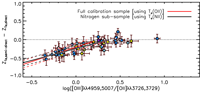
Given the findings above, we here derive an empirical correction to the semi-direct $Z_{\textnormal{Te}}$ deficit using the easily-observable ratio of oxygen nebular lines, $[\textnormal{{Oiii}}]$$\lambda\lambda 4959,5007$/$[\textnormal{{Oii}}]$$\lambda\lambda 3726,3729$ [see panel (b) of Fig. 7]. A linear fit to this relation yields a correction factor, $f_{\textnormal{cor}}$, given by,

$$f_{\textnormal{cor}}=\bigg{\{} \begin{array}[]{ll}0.77\,(x-0.20)&\textnormal{for }x\leq 0.26\\ 0.0&\textnormal{for }x>0.26\end{array}\;\;\;\;\textnormal{\footnotesize{(Least squares)}}\;\;,$$ (14)

$$f_{\textnormal{cor}}=\bigg{\{} \begin{array}[]{ll}0.71\,(x-0.29)&\textnormal{for }x\leq 0.29\\ 0.0&\textnormal{for }x>0.29\end{array}\;\;\;\;\textnormal{\footnotesize{(Bayesian)}}\;\;,$$ (17)

where $x=\textnormal{log($[\textnormal{{Oiii}}]${}}\lambda\lambda 4959,5007/\textnormal{$[\textnormal{{Oii}}]${}}\lambda\lambda 3726,3729)$. The corrected semi-direct oxygen abundance is therefore given by,

$$Z_{\textnormal{Te,cor}}=\textnormal{$Z_{\textnormal{Te}}${}}-f_{\textnormal{cor}}\;\;.$$ (18)

Figure 11: Mass-metallicity relation for the 118 galaxies in our dataset. Galaxies are coloured according to the sample from which their fluxes were taken. Points with thick black rings have direct $Z_{\textnormal{Te}}$ estimates [i.e. $T_{\textnormal{e}}(\textnormal{{Oiii}})$ and $T_{\textnormal{e}}(\textnormal{{Oii}})$ independently calculated], while the remaining points have semi-direct $Z_{\textnormal{Te}}$ estimates, i.e. using our new semi-direct method, corrected for the observed $\textnormal{O}^{++}$/$\textnormal{O}^{+}$ bias using our least-squares-derived $f_{\textnormal{cor}}$ (see §5.3). The least-squares and Bayesian linear fits to all the points (Eq. 6) are shown by the solid black line and solid dark grey line, respectively, with the 1$\sigma$ dispersions given by dashed lines.

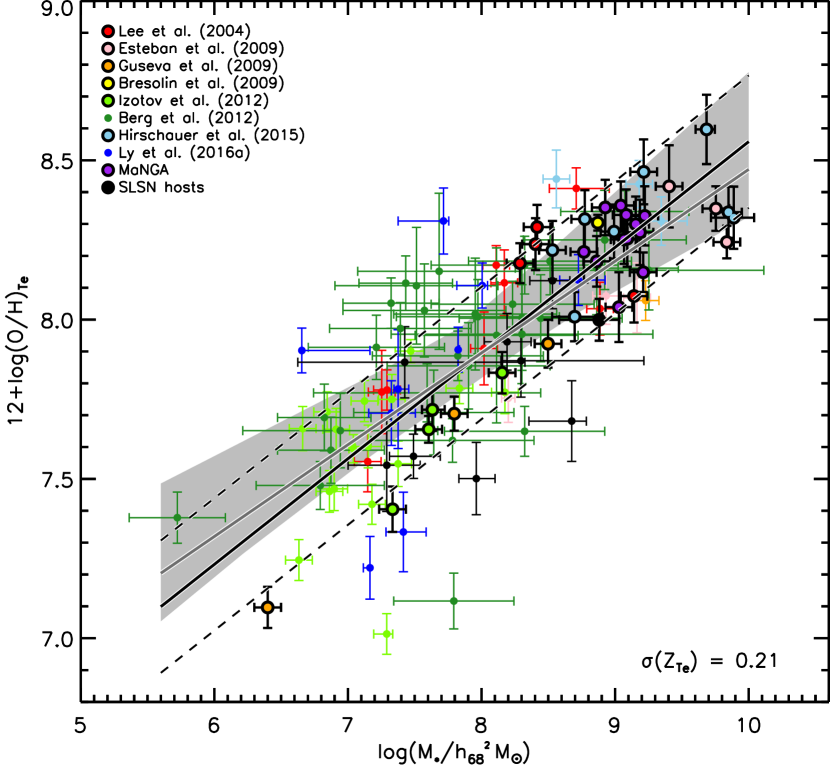
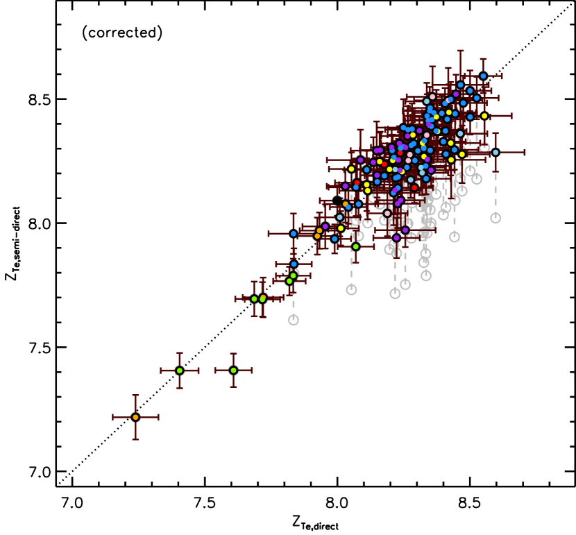
Fig. 8 shows the comparison between direct $Z_{\textnormal{Te}}$ and the corrected semi-direct $Z_{\textnormal{Te}}$ using our new $T_{\textnormal{e}}(\textnormal{{Oiii}})$ – $T_{\textnormal{e}}(\textnormal{{Oii}})$ relation. There is now a much more consistent correspondence between these two methods across a large range of oxygen abundances. However, despite this clear improvement, we do caution that empirical corrections of this nature do not directly relate the physics linking the two variables in question to the discrepancy observed and are, therefore, liable to provide spurious corrections when applied to inappropriate systems.

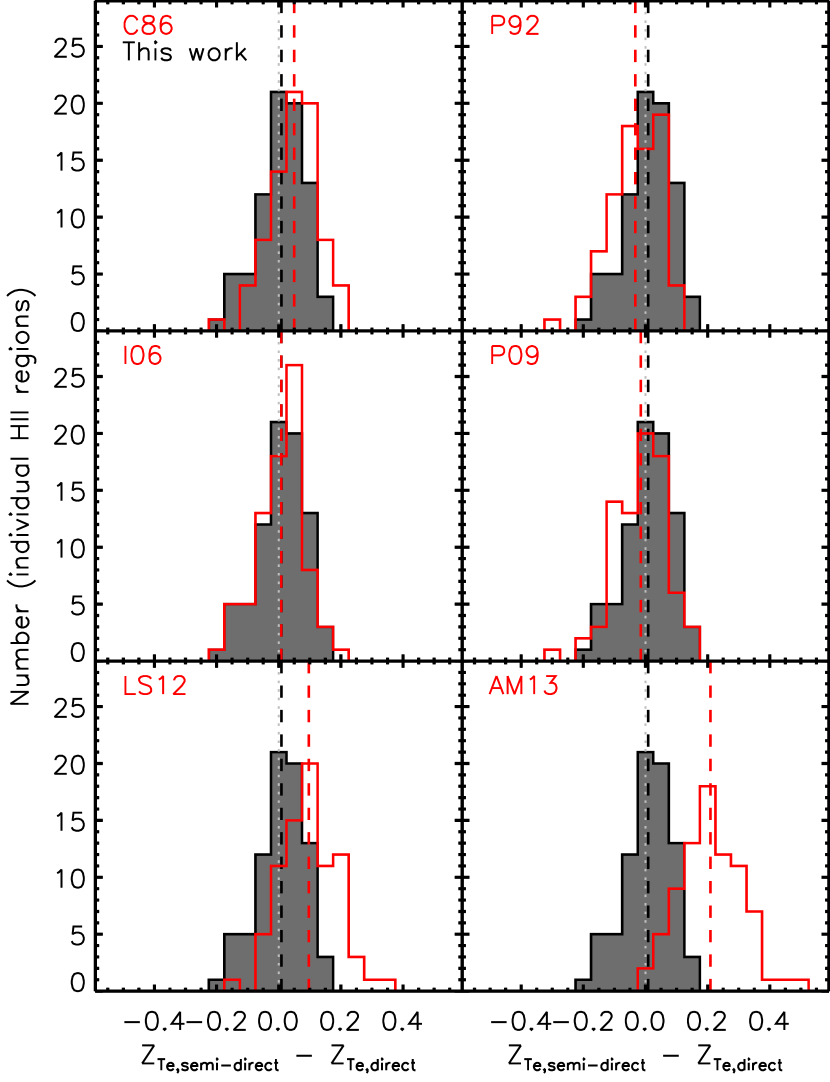
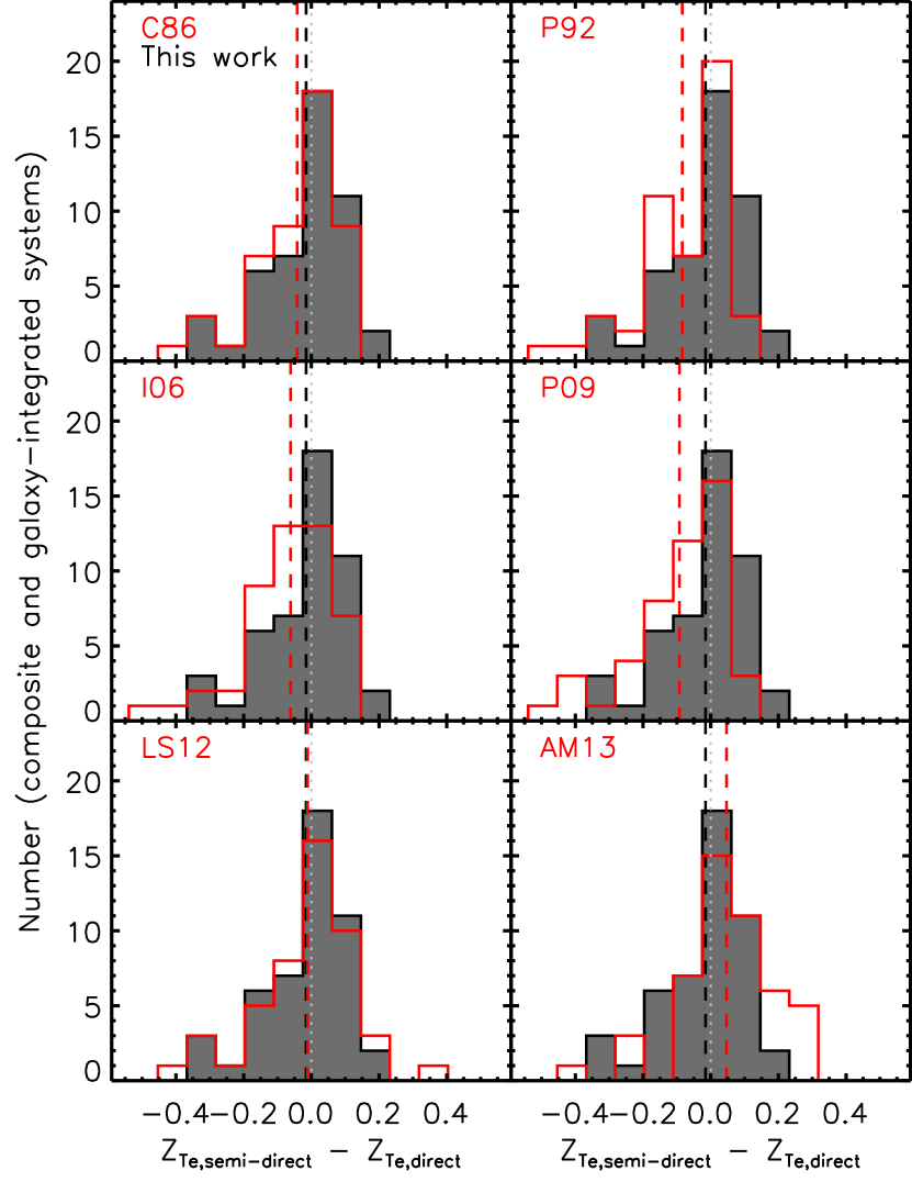
We also compare the accuracy of our new semi-direct method with those from the literature. We do this by splitting our sample into individual Hii region spectra and composite/integrated-galaxy spectra (as defined in §5.2.4), and plotting the semi-direct $Z_{\textnormal{Te}}$ deficit distributions from each semi-direct method separately for these two sub-samples in Figs. 9 and 10. These figures clearly show that those literature relations calibrated to single Hii regions (e.g. Izotov et al. 2006 or Pilyugin et al. 2009) perform relatively well for our individual Hii region spectra, but poorly for composite and global spectra. Conversely, those relations calibrated to composite Hii regions (e.g. López-Sánchez et al. 2012 or Andrews & Martini 2013) perform relatively well for our composite or integrated-galaxy spectra, but poorly for the highly-resolved systems. Our new relation, on the other hand, calibrated to a varied dataset, works equally well for all systems of any physical size, with a mean semi-direct $Z_{\textnormal{Te}}$ deficit of almost zero in both cases.

When using our dataset as a whole, the standard deviation around the peak of the distribution for our new semi-direct method is 0.08 dex, and there are no systems with $Z_{\textnormal{Te}}$ discrepancies greater than $-0.35$ dex, regardless of their ionisation state.

6 The local MZR

In Fig. 11, we plot the $M_{*}$-$Z_{\textnormal{Te}}$ relation (MZR) for the 118 galaxies that make up our dataset. These galaxies contain the 130 individual and composite Hii regions discussed in the preceding sections, as well as additional systems for which semi-direct $Z_{\textnormal{Te}}$ estimates can be obtained. For galaxies with electron temperature measurements for more than one Hii region, the H$\alpha$-flux-weighted mean $Z_{\textnormal{Te}}$ is used, except for our MaNGA galaxies for which the $Z_{\textnormal{Te}}$ obtained from the global spectra are used. Points with thick black outlines in Fig. 11 represent galaxies with direct $Z_{\textnormal{Te}}$ estimates, while the other points represent galaxies with our semi-direct $Z_{\textnormal{Te}}$ estimates.

Our new MZR represents an improvement on previous $T_{\textnormal{e}}$-based relations in the literature predominantly because (a) our dataset is not biased to strongly star-forming systems, and (b) we have corrected for the semi-direct $Z_{\textnormal{Te}}$ deficit in low-$\textnormal{O}^{++}$/$\textnormal{O}^{+}$ systems discussed in §5.2 and §5.3.

We find the following linear fit to our MZR, using our least-squares and Bayesian analyses:

$$Z_{\textnormal{Te}} =0.332\textnormal{\scriptsize{$\pm 0.021$}}\;\textnormal{log}(M_{*})+5.242\textnormal{\scriptsize{$\pm 0.171$}} \textnormal{\footnotesize{(Least squares)}}\;,$$

$$Z_{\textnormal{Te}} =0.293\textnormal{\scriptsize{$\pm 0.023$}}\;\textnormal{log}(M_{*})+5.575\textnormal{\scriptsize{$\pm 0.192$}} \textnormal{\footnotesize{(Bayesian)}}\;,$$ (19)

in the range $5.67<\textnormal{log}(M_{*})<9.87$, where $M_{*}$ is in units of $h^{2}_{68}\,\textnormal{M}_{\textnormal{\astrosun}}$. The 1$\sigma$ dispersion in $Z_{\textnormal{Te}}$ is 0.21 dex for the least-squares fit from residuals. This spread is larger than the 1$\sigma$ dispersion of $\sim 0.10$ dex obtained from most strong-line-based MZRs (e.g. Tremonti et al. 2004; Yates et al. 2012), suggesting that the local MZR has a wider scatter than usually assumed. The scatter above our relation is partly due to our low-$[\textnormal{{Oiii}}]$/$[\textnormal{{Oii}}]$ correction to semi-direct $Z_{\textnormal{Te}}$ estimates (see §5.3). For example, the Berg et al. (2012) system CGCG035-007A with log$(M_{*}/h_{68}^{2}\,\textnormal{M}_{\textnormal{\astrosun}})=7.51$ and $Z_{\textnormal{Te}}$$=8.11$ has a low log($[\textnormal{{Oiii}}]$/$[\textnormal{{Oii}}]$) ratio of -0.14, which has caused a $Z_{\textnormal{Te}}$ correction upwards by $\sim{}0.31$ dex. However, the other systems close to CGCG035-007A on the MZR actually have relatively high log($[\textnormal{{Oiii}}]$/$[\textnormal{{Oii}}]$) ratio, so their high $Z_{\textnormal{Te}}$ estimates are not due to any correction. We find the scatter below the MZR is driven by unusually-high electron temperatures. For example, the low-metallicity outlier, UGC5340A from the Berg et al. (2012) sample (which is believed to be undergoing a merger), has measured $T_{\textnormal{e}}(\textnormal{{Oiii}})$ $=18830$ K and $T_{\textnormal{e}}(\textnormal{{Oii}})$ $=20359$ K, leading to $Z_{\textnormal{Te}}$ $=7.12$.

Figure 12: Comparison between our new $T_{\textnormal{e}}$-based MZR (solid black line, Eq. 6) and various strong-line-based MZRs presented by Kewley & Ellison (2008, dotted lines). As for many other $Z_{\textnormal{Te}}$ studies, we find a lower normalisation for our MZR compared to the strong-line-based relations, although the slope is quite similar among most cases below $\textnormal{log(}M_{*}/\,\textnormal{M}_{\textnormal{\astrosun}})\sim{}10.0$.

Figure 13: Comparison between our new $T_{\textnormal{e}}$-based MZR $T_{\textnormal{e}}$-based MZR (solid black line, Eq. 6) and other recent $T_{\textnormal{e}}$-based MZRs from the literature. Fits to the relations from Lee et al. (2006, orange), Andrews & Martini (2013, green), Izotov et al. (2015, light blue), and Ly et al. (2016b, dark blue) are shown. Stellar masses have been corrected for differences in the assumed dimensionless Hubble parameter where possible.

6.1 Comparison with other MZRs

6.1.1 Strong-line MZRs

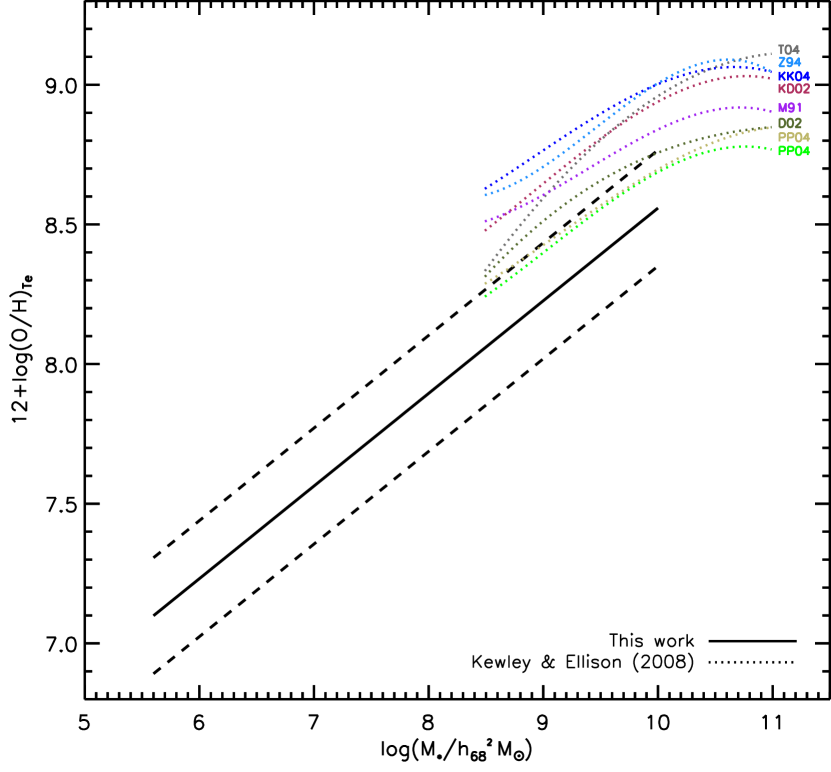
In Fig. 12, our MZR is shown alongside fits to the MZRs from the various strong-line metallicity diagnostics presented by Kewley & Ellison (2008). Our new $T_{\textnormal{e}}$-based MZR has a lower normalisation at fixed mass than MZRs based on strong lines, by $0.15-0.55$ dex at $\textnormal{log}(M_{*}/\,\textnormal{M}_{\textnormal{\astrosun}})\sim 9.0$, although the slopes are found to be similar.

A lower normalisation for $T_{\textnormal{e}}$-based MZRs has been seen many times before (e.g. Stasińska 2005; Lee et al. 2006; Andrews & Martini 2013; Ly et al. 2014; Izotov et al. 2015). This is unlikely to be caused by a preferential selection of low-metallicity systems at fixed mass in our case because our dataset contains a significant contribution of typically star-forming systems (see §3). We therefore concur with most previous studies that the oxygen abundance in the ISM of low-redshift galaxies is lower than indicated by traditional strong-line diagnostics applied to large star-forming galaxy samples such as the SDSS.

Our findings are qualitatively consistent with the fundamental metallicity relation (FMR, Mannucci et al. 2010), although we are unable to draw any firm conclusions on the anti-correlation between $Z_{\textnormal{Te}}$ and SFR at low-mass, due to the relatively low number of systems at fixed mass and metallicity. We do, however, find a clear increase in star-formation rate (SFR) with both $Z_{\textnormal{Te}}$ and $M_{*}$ for our dataset.

6.1.2 $T_{\textnormal{e}}$-based MZRs

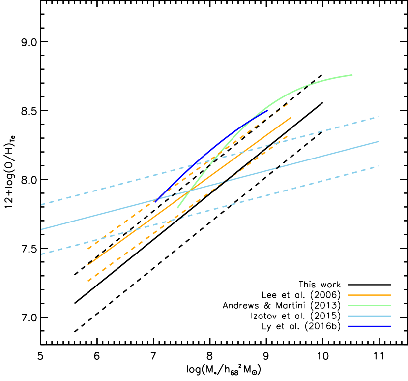
Fig. 13 compares our new MZR (black solid line) with those from other recent studies of $T_{\textnormal{e}}$-based metallicities using different samples.

Our MZR appears to be in best agreement with that of Lee et al. (2006), who utilised Spitzer IR photometry to determine stellar masses and a variety of different semi-direct $T_{\textnormal{e}}$-based metallicities from the literature for their smaller sample of 27 dwarf irregular galaxies. We determine a larger scatter around the MZR for our larger sample of 118 galaxies, and a lower normalisation.

The slope of the MZR derived by Izotov et al. (2015) (light blue) for 3607 star-forming galaxies from the SDSS-DR7 is significantly shallower than the other $T_{\textnormal{e}}$-based MZRs considered here. This is likely due to the different sample selection criteria applied. Izotov et al. (2015) selected compact ($R_{50}<6$ arcsec) galaxies with high nebular excitation as given by log($[\textnormal{{Oiii}}]$$\lambda 5007/\textnormal{H}\beta)\gtrsim 0.5$. They also required a detection of the auroral $[\textnormal{{Oiii}}]$$\lambda 4363$ line from the relatively shallow SDSS spectroscopy in order to estimate $T_{\textnormal{e}}(\textnormal{{Oiii}})$. These criteria all limit the number of higher-metallicity galaxies in their sample at higher mass, effectively selecting systems with similar physical conditions to higher-redshift galaxies. This is likely causing the lower typical metallicities seen in the Izotov et al. (2015) sample above $\textnormal{log}(M_{*}/\,\textnormal{M}_{\textnormal{\astrosun}})\sim 8.0$, and therefore the shallower slope compared to other works.

The MZR from Andrews & Martini (2013) has a normalisation $\sim{}0.3$ dex higher than ours at $\textnormal{log}(M_{*}/\,\textnormal{M}_{\textnormal{\astrosun}})\sim{}9.0$. Their study utilised $T_{\textnormal{e}}$ measurements from stacked SDSS-DR7 spectra, containing around 2,000 galaxies in each bin at $\textnormal{log}(M_{*}/\,\textnormal{M}_{\textnormal{\astrosun}})\sim{}9.0$.

Although Fig. 9 shows that the $T_{\textnormal{e}}(\textnormal{{Oiii}})$ – $T_{\textnormal{e}}(\textnormal{{Oii}})$ relation fit to the Andrews & Martini (2013) data returns semi-direct $Z_{\textnormal{Te}}$ estimates around 0.2 dex higher than our relation, we note that this is the case when applied to spectra of individual Hii regions. For the more global galaxy spectra that make up the bulk of our MZR, we actually find a relatively close correspondence between the $Z_{\textnormal{Te}}$ estimated via the AM13 relation and our own (see also Fig. 10).

The range of SFRs found in each sample at $\textnormal{log}(M_{*}/\,\textnormal{M}_{\textnormal{\astrosun}})\sim{}9.0$ are also similar, with $-1.0<\textnormal{log(SFR}/\,\textnormal{M}_{\textnormal{\astrosun}}\,\textnormal{yr}^{-1})<0.0$ in both cases. It is therefore unlikely that differences in the $T_{\textnormal{e}}(\textnormal{{Oiii}})$ – $T_{\textnormal{e}}(\textnormal{{Oii}})$ relations or sample selection biases are responsible for the MZR normalisation difference seen here.

Rather, the predominant cause is likely differences in the estimated direct $\textnormal{O}^{+}/\textnormal{H}^{+}$ obtained from each analysis; Andrews & Martini (2013) find a value of $12+\textnormal{log($\textnormal{O}^{+}/\textnormal{H}^{+}${})}\sim{}8.5$ for their $\textnormal{log}(M_{*}/\,\textnormal{M}_{\textnormal{\astrosun}})\sim{}9.0$ stack (their fig. 5), compared to values between 7.2 and 8.4 for our direct $Z_{\textnormal{Te}}$ systems of a similar mass. $\textnormal{O}^{++}/\textnormal{H}^{+}$ estimates at fixed mass, on the other hand, are more similar between the two studies.

The higher $\textnormal{O}^{+}/\textnormal{H}^{+}$ estimates they obtain could be partly due to the composite spectra issue discussed by Pilyugin et al. (2010) (see §5.2.4). However this is unlikely to explain the entire difference in $Z_{\textnormal{Te}}$ seen, as stacked spectra should not be more prone to such issues than global spectra of individual galaxies (Pilyugin et al., 2010; Andrews & Martini, 2013; Curti et al., 2017). Limitations with the assumption that galaxies of the same stellar mass should have similar metallicities (see Curti et al. 2017), as well as SDSS fibre aperture effects (see Ellison et al. 2008), could also play a role.

Finally, the results presented by Ly et al. (2016b) on the low-redshift MZR from the Metal Abundances Across Cosmic Time (MACT) survey also suggests higher metallicities than most other $T_{\textnormal{e}}$-based MZRs considered here. Although $\textnormal{O}^{++}/\textnormal{H}^{+}$ abundances were determined in a very similar way to our methodology, the lack of direct $\textnormal{O}^{+}/\textnormal{H}^{+}$ measurements and reliance on the $T_{\textnormal{e}}(\textnormal{{Oiii}})$ – $T_{\textnormal{e}}(\textnormal{{Oii}})$ relation calibrated to the Andrews & Martini (2013) stacked data is likely causing the higher normalisation, as discussed above.

Figure 14: Fit to our $T_{\textnormal{e}}$-based MZR (solid black line, Eq. 6), plotted alongside the MZR from oxygen recombination lines (yellow/orange points, Esteban et al. 2009, 2014), the MZR from blue supergiant star photospheres (blue points, Kudritzki et al. 2016), and the MZR from the integrated stellar populations of SDSS-DR7 star-forming galaxies (red points, Zahid et al. 2017).

6.1.3 Alternative direct methods

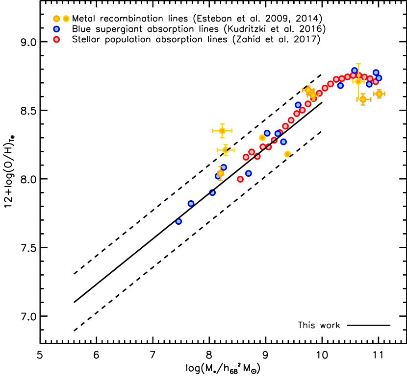
In Fig. 14, the fit to our low-redshift MZR given by Eq. 6 is shown (black line), compared to MZRs formed using the two methods for obtaining gas-phase oxygen abundances that are generally considered to be most accurate. Large yellow points denote 10 nearby ($z<0.023$) galaxies for which O/H has been calculated in the brightest Hii regions from faint metal recombination lines by Esteban et al. (2009) and Esteban et al. (2014). Large blue points denote 15 galaxies for which O/H has been calculated from absorption lines in the photospheres of blue supergiant stars by Kudritzki et al. (2016, and references therein), taking the metallicity at two disc scale lengths from the measured blue-supergiant abundance gradient.

Stellar masses for the Esteban et al. (2009, 2014) samples are taken from the literature (Sick et al. 2014; Lelli et al. 2014; van Dokkum et al. 2014; López-Sánchez 2010; Skibba et al. 2011; Östlin et al. 2003; Woo et al. 2008; and the NSA catalogue). Stellar masses for the Kudritzki et al. (2016) sample are taken from various other works, as listed in table 4 of Kudritzki et al. (2012). Where possible, we have ensured that these are corrected for any differences in the assumed IMF or cosmology.

A key finding of this study is that there is remarkably good agreement between the MZR formed from our new $T_{\textnormal{e}}$ analysis and those formed from metal recombination lines and blue supergiant absorption lines. There has been long-standing evidence that $T_{\textnormal{e}}$ methods typically under-predict the $\textnormal{O}^{++}/\textnormal{H}^{+}$ abundance by $0.26-0.43$ dex compared to RL methods for the same individual Hii regions (Esteban et al. 2009, 2014). However, it appears from Fig. 14 that, in an overall sense, our $T_{\textnormal{e}}$-based MZR is consistent with that formed using RLs and stellar absorption-line spectra.

Additionally, Zahid et al. (2017) have also produced an MZR based on stacked absorption-line spectra from the SDSS-DR7, using sequential single-burst (SSB) SPS models. Their luminosity-weighted MZR is also plotted in Fig. 14 as red points. There is also very good agreement between the Zahid et al. (2017) MZR and those of Kudritzki et al. (2016), Esteban et al. (2009, 2014), and this work. This convergence of various different direct metallicity methods on a consistent MZR is a promising sign than the true metal content of nearby galaxies is being correctly probed by our new analysis.

7 Summary & Conclusions

Electron temperatures ($T_{\textnormal{e}}$) and gas-phase oxygen abundances ($Z_{\textnormal{Te}}$) have been obtained for 264 emission-line systems in the local Universe ($z<0.25$). This dataset comprises a mix of individual, composite, and whole-galaxy spectra, belonging to both starbursting galaxies and galaxies on the star-forming main sequence. The 130 systems with direct measurements of both $T_{\textnormal{e}}(\textnormal{{Oiii}})$ and $T_{\textnormal{e}}(\textnormal{{Oii}})$ are utilised to calibrate a new $T_{\textnormal{e}}(\textnormal{{Oiii}})$ – $T_{\textnormal{e}}(\textnormal{{Oii}})$ relation, which can be used to estimate $Z_{\textnormal{Te}}$ using the $[\textnormal{{Oiii}}]$$\lambda 4363$ auroral line. The resulting mass – metallicity relation (MZR) for 118 low-redshift, star-forming galaxies with $5.5\lesssim\textnormal{log}(M_{*}/\,\textnormal{M}_{\textnormal{\astrosun}})\lesssim 10.0$ is then compared to previous works. Our key findings and conclusions are as follows:

• Due to its hyperbolic functional form, our new metallicity-dependent $T_{\textnormal{e}}(\textnormal{{Oiii}})$ – $T_{\textnormal{e}}(\textnormal{{Oii}})$ relation (Eq. 5.1) allows for a wider range of $T_{\textnormal{e}}(\textnormal{{Oii}})$/$T_{\textnormal{e}}(\textnormal{{Oiii}})$ ratios than previous relations. The semi axis of the hyperbola is tightly constrained by $Z_{\textnormal{Te}}$ (see §5.1). Both $T_{\textnormal{e}}(\textnormal{{Oii}})$ and $Z_{\textnormal{Te}}$ can therefore be obtained iteratively for any system with a robust $[\textnormal{{Oiii}}]$$\lambda{}4363$ auroral line detection.

• We find that all the literature $T_{\textnormal{e}}(\textnormal{{Oiii}})$ – $T_{\textnormal{e}}(\textnormal{{Oii}})$ relations considered here, as well as our own, underestimate $Z_{\textnormal{Te}}$ for systems with log($\textnormal{O}^{++}$/$\textnormal{O}^{+}$) $\lesssim 0.0$ (see Fig. 7a). After investigating the possible causes for this semi-direct $Z_{\textnormal{Te}}$ deficit, we determine that it is most likely due to the physical dominance of $\textnormal{O}^{+}$ ions over $\textnormal{O}^{++}$ in the Hii regions of these systems, making $Z_{\textnormal{Te}}$ estimates difficult to obtain from measurements of $T_{\textnormal{e}}(\textnormal{{Oiii}})$ alone (see §5.2).

• We therefore provide an empirically-calibrated correction to our semi-direct $Z_{\textnormal{Te}}$ estimates for low-$\textnormal{O}^{++}$/$\textnormal{O}^{+}$ systems, based on the easily-observable nebular oxygen line ratio $[\textnormal{{Oiii}}]$/$[\textnormal{{Oii}}]$. Our new method can then return accurate $Z_{\textnormal{Te}}$ estimates for systems of either high or low ionisation, regardless of their spatial resolution. Overall, our semi-direct $Z_{\textnormal{Te}}$ estimates are within a standard deviation of 0.08 dex from the directly-measured values, which is comparable to or better than any of the literature $T_{\textnormal{e}}(\textnormal{{Oiii}})$ – $T_{\textnormal{e}}(\textnormal{{Oii}})$ relations considered here (see Figs. 9 and 10).

• The low-redshift MZR formed using our new $Z_{\textnormal{Te}}$ estimates has a similar slope to most strong-line based MZRs but a lower normalisation, as found by most previous studies (see §6.1.1). The scatter of $\sigma{}(\textnormal{$Z_{\textnormal{Te}}$})\sim{}0.21$ we find is larger than is typically found when using strong-line diagnostics.

• When comparing to other $T_{\textnormal{e}}$-based MZRs, we deduce that any differences are mainly due to sample selection biases or differences in the direct determination of $\textnormal{O}^{+}/\textnormal{H}^{+}$, rather than the particular $T_{\textnormal{e}}(\textnormal{{Oiii}})$ – $T_{\textnormal{e}}(\textnormal{{Oii}})$ relation used when obtaining semi-direct $Z_{\textnormal{Te}}$ estimates. The inclusion of many ‘star-forming main sequence’ galaxies in our dataset makes our MZR more representative of the typically-star-forming population at low redshift.

• Encouragingly, our new $T_{\textnormal{e}}$-based MZR is in very good agreement with the MZRs obtained via direct metallicity measurements from metal recombination lines or blue supergiant absorption lines (see §6.1.3). This is a strong indication that our study is accurately probing the true range of metallicities present in the star-forming galaxy population at low redshift.

In a follow-up paper, we will compare our new $T_{\textnormal{e}}$-based MZR with MZRs derived from alternative direct methods at higher redshifts, in order to ascertain the true evolution of the gas-phase metallicity in galaxies over cosmic time.

Appendix A An alternative nitrogen-based calibration

In addition to the calibration of our new $T_{\textnormal{e}}(\textnormal{{Oiii}})$ – $T_{\textnormal{e}}(\textnormal{{Oii}})$ relation presented in §5.1, we also present here a complimentary calibration to the $T_{\textnormal{e}}(\textnormal{{Oiii}})$ – $T_{\textnormal{e}}(\textnormal{{Nii}})$ relation, using a subset of 53 systems (hereafter, the ‘nitrogen sub-sample’) for which measurements of both the $[\textnormal{{Oiii}}]$$\lambda 4363$ and $[\textnormal{{Nii}}]$$\lambda 5755$ auroral lines are available.

$[\textnormal{{Nii}}]$$\lambda 5755$ is a particularly weak auroral line, with a mean S/N of only 8.2 for our nitrogen sub-sample, compared to S/N($[\textnormal{{Oiii}}]$$\lambda 4363)=17.4$ and S/N($[\textnormal{{Oii}}]$$\lambda\lambda 7320,7330)=27.3$ for the same systems. Nonetheless, due to the similar ionisation energies required for $[\textnormal{{Oii}}]$ and $[\textnormal{{Nii}}]$, both are expected to trace the same ionisation zone within an Hii region, and return similar electron temperatures. Therefore, $T_{\textnormal{e}}(\textnormal{{Nii}})$ can be a useful alternative to $T_{\textnormal{e}}(\textnormal{{Oii}})$ when estimating $\textnormal{O}^{+}$, in cases where $[\textnormal{{Oii}}]$$\lambda\lambda 7320,7330$ is not available or believed to be contaminated (see §5.2.2).

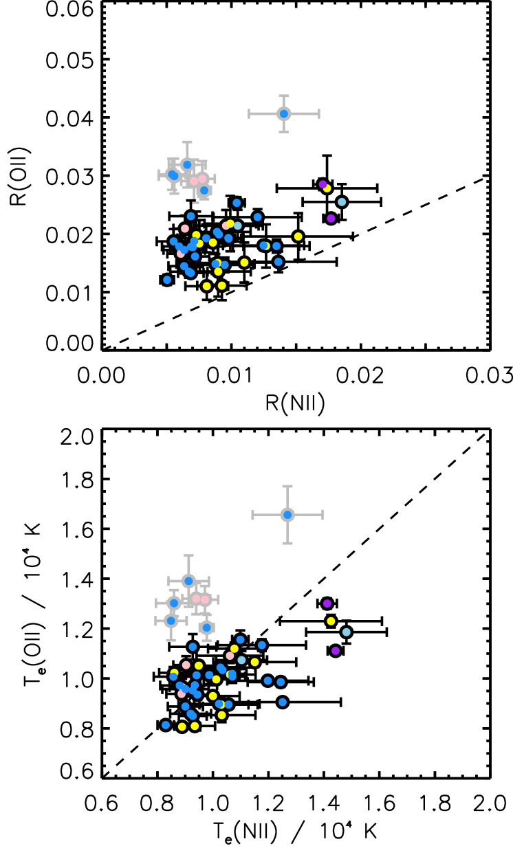
Fig. 15 shows the R(Nii) - R(Oii) relation and $T_{\textnormal{e}}(\textnormal{{Nii}})$ - $T_{\textnormal{e}}(\textnormal{{Oii}})$ relation for our nitrogen sub-sample. With the exception of a few systems with unexpectedly high R(Oii) and $T_{\textnormal{e}}(\textnormal{{Oii}})$ (outlined in grey), we find a good linear relationship between these line ratios and temperatures, with a median difference between $T_{\textnormal{e}}(\textnormal{{Oii}})$ and $T_{\textnormal{e}}(\textnormal{{Nii}})$ of only 165 K. In particular, the good one-to-one correspondence between $T_{\textnormal{e}}(\textnormal{{Oii}})$ and $T_{\textnormal{e}}(\textnormal{{Nii}})$ for the CHAOS sample (blue points) is a clear improvement on that reported by the original works (Berg et al. 2015; Croxall et al. 2016). This is because we estimate higher $T_{\textnormal{e}}(\textnormal{{Nii}})$ at fixed $T_{\textnormal{e}}(\textnormal{{Oii}})$ than those studies, bringing these two temperatures more in line with each other.

The $T_{\textnormal{e}}(\textnormal{{Oiii}})$ – $T_{\textnormal{e}}(\textnormal{{Nii}})$ relation is shown in the top panel of Fig. 16. There are fewer systems with large differences between these temperatures than seen for the $T_{\textnormal{e}}(\textnormal{{Oiii}})$ – $T_{\textnormal{e}}(\textnormal{{Oii}})$ relation of our full calibration sample (see Fig. 2). The lack of systems in the upper part of this plane (i.e. in region A of the schematic shown in Fig. 3) is mainly due to measured $T_{\textnormal{e}}(\textnormal{{Nii}})$ being lower than $T_{\textnormal{e}}(\textnormal{{Oii}})$ for those systems (outlined in grey in Fig. 15). The lack of systems in the lower part of this plane (i.e. region B in Fig. 3) is chiefly a selection bias: systems with higher metallicity have particularly weak $[\textnormal{{Nii}}]$$\lambda 5755$, and are therefore typically removed from samples selected on this line.

Figure 15: Top panel: Relation between $R(\textnormal{N{ii}})=[\textnormal{N{ii}}]\lambda 5755/(1.33\cdot{}\textnormal{N{ii}}]\lambda 6584)$ and $R(\textnormal{O{ii}})=[\textnormal{O{ii}}]\lambda\lambda 7320,7330/[\textnormal{O{ii}}]\lambda\lambda 3726,3729$, for our nitrogen sub-sample of 53 systems. Bottom panel: Relation between $T_{\textnormal{e}}(\textnormal{{Nii}})$ and $T_{\textnormal{e}}(\textnormal{{Oii}})$ for the same nitrogen sub-sample. These two temperatures are expected to be roughly the same for a given Hii region, as indicated by the line of equality (dashed line). Points with grey outlines (in both panels) are outliers with $T(\textnormal{{Oii}})>T(\textnormal{{Nii}})+2000$ K, or equivalently, $R(\textnormal{{Oii}})>R(\textnormal{{Nii}})+0.0175$ K.

Figure 16: Top panel: $T_{\textnormal{e}}(\textnormal{{Oiii}})$ – $T_{\textnormal{e}}(\textnormal{{Nii}})$ relation for our nitrogen sub-sample of 53 systems (points). Fits to the $T_{\textnormal{e}}(\textnormal{{Oiii}})$ – $T_{\textnormal{e}}(\textnormal{{Oii}})$ relation from the literature are also shown. Centre panel: The relation between direct $Z_{\textnormal{Te}}$ and the hyperbolic semi-axis, $a$. Red lines indicate the least-squares fit to our full calibration sample, using $T_{\textnormal{e}}(\textnormal{{Oii}})$ (see Eq. 5.1). Black lines indicate the least-squares fit to our nitrogen sub-sample when using $T_{\textnormal{e}}(\textnormal{{Nii}})$. Bottom panel: Relation between the semi-direct $Z_{\textnormal{Te}}$ deficit and $[\textnormal{{Oiii}}]$/$[\textnormal{{Oii}}]$. Again, red lines denote our least-squares $[\textnormal{{Oii}}]$-based fit (see Fig. 7), black lines denote our least-squares alternative $[\textnormal{{Nii}}]$-based fit.

The centre panel of Fig. 16 shows the $Z_{\textnormal{Te}}$ – $a$ relation. The red lines represent the least-squares fit for our full calibration sample, as shown in Fig. 4. We find there is very little difference in the fit obtained when removing those systems that have $T(\textnormal{{Oii}})>T(\textnormal{{Nii}})+2000$ K (shown with grey outlines in Fig. 15). This further demonstrates that our new calibration performs well for systems on and off the expected relations for individual Hii regions.

The black lines in the centre panel of Fig. 16 represent the least-squares fit to our nitrogen sub-sample when using $T_{\textnormal{e}}(\textnormal{{Nii}})$ to obtain $\textnormal{O}^{+}/\textnormal{H}^{+}$. This relation is steeper than that using $T_{\textnormal{e}}(\textnormal{{Oii}})$ to obtain $\textnormal{O}^{+}/\textnormal{H}^{+}$. The steepness is driven by the small number of systems with $a\gtrsim 17000$, which have higher measured $T_{\textnormal{e}}(\textnormal{{Nii}})$ than $T_{\textnormal{e}}(\textnormal{{Oii}})$. It is important to note that all these systems have $\textnormal{log($\textnormal{O}^{++}${}/$\textnormal{O}^{+}${})}>0.5$, so are relatively insensitive to how $\textnormal{O}^{+}$ is estimated anyway. The majority of the $T_{\textnormal{e}}(\textnormal{{Nii}})$ sub-sample is still well fit by our $[\textnormal{{Oii}}]$-based calibration. Also, the semi-direct $Z_{\textnormal{Te}}$ deficit correction we derive is very similar for both the full calibration sample and nitrogen sub-sample (bottom panel). Nonetheless, we still provide the revised least-squares fits to our hyperbolic semi axis, $a$, and correction factor, $f_{\textnormal{cor}}$, when using $T_{\textnormal{e}}(\textnormal{{Nii}})$:

$$a_{\textnormal{N{ii}}}= -19649.06\textnormal{\scriptsize{$\pm 2504.29$}}\;\textnormal{$Z_{\textnormal{Te}}${}}+177133.93\textnormal{\scriptsize{$\pm 20827.90$}}\;\;,$$ (20)

$$f_{\textnormal{cor,N{ii}}}=\bigg{\{} \begin{array}[]{ll}0.64\,(x-0.24)&\textnormal{for }x\leq 0.37\\ 0.0&\textnormal{for }x>0.37\end{array}\;\;.$$ (23)

As with our $[\textnormal{{Oii}}]$-based calibration, our $[\textnormal{{Nii}}]$-based calibration returns relatively accurate $Z_{\textnormal{Te}}$ estimates for the full range of systems available (as discussed in 5.3).

Appendix B MaNGA EW(H$\alpha$) maps and tables

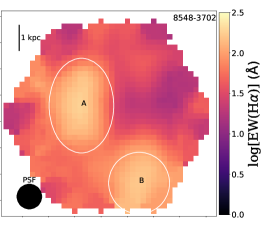
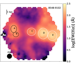
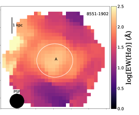
In Fig. 17, we present the H$\alpha$ EW maps for our sample of MaNGA galaxies (see §2). White ellipses signify Hii blobs with S/N$[\textnormal{{Oiii}}]$$\lambda{}4363\geq 3.0$. All spaxels within an ellipse with EW(H$\alpha$) $>50$Å and S/N(H$\alpha$) $>50$ are used to determine emission line fluxes. Table LABEL:tab:MaNGA_HIIblob_data provides the emission line intensities measured for each of the MaNGA Hii blobs in our sample, along with their derived electron temperatures and oxygen abundances. Table 2 provides similar data from our global MaNGA galaxy spectra, and includes information on their position, stellar mass, extinction, and electron density.

Figure 17: EW(H$\alpha$) maps for the 12 galaxies from our MaNGA sample containing Hii blobs with auroral line detections (see §2). Hii blobs are shown and numbered in each panel. White ellipses signify Hii blobs with S/N$[\textnormal{{Oiii}}]$$\lambda{}4363\geq 3.0$, which are used for our $T_{\textnormal{e}}$ analysis in §4.3.

Table 1: Fluxes in units of $10^{-15}$ erg s^-1 cm², corrected for Galactic foreground extinction, for the 24 Hii blobs with S/N([Oiii]$\lambda$4363) $\geq 3.0$ from our MaNGA galaxies. Electron densities, temperatures, and oxygen abundances are also provided.

System	7495-6102B	7495-6102C	7495-6102D	8133-3704A	8133-3704B	8252-12701A
$[$Oii]$\lambda$3726	14.77$\pm$0.24	1.68$\pm$0.05	1.42$\pm$0.03	2.50$\pm$0.04	3.13$\pm$0.03	1.02$\pm$0.01
$[$Oii]$\lambda$3729	21.81$\pm$0.24	2.43$\pm$0.05	2.09$\pm$0.03	3.73$\pm$0.04	5.22$\pm$0.03	1.60$\pm$0.01
$[$Sii]$\lambda$4073	0.09$\pm$0.03	0.01$\pm$0.01	–	0.05$\pm$0.04	0.02$\pm$0.03	–
$[$Oiii]$\lambda$4363	0.34$\pm$0.03	0.03$\pm$0.01	0.03$\pm$0.01	0.14$\pm$0.04	0.09$\pm$0.01	0.05$\pm$0.01
H$\beta\ \lambda$4861	14.79$\pm$0.05	1.38$\pm$0.01	1.26$\pm$0.02	3.08$\pm$0.04	2.87$\pm$0.02	0.96$\pm$0.01
$[$Oiii]$\lambda$4959	16.99$\pm$0.05	1.28$\pm$0.01	1.37$\pm$0.01	4.90$\pm$0.05	2.77$\pm$0.01	1.03$\pm$0.01
$[$Oiii]$\lambda$5007	48.39$\pm$0.22	3.71$\pm$0.02	4.08$\pm$0.02	14.09$\pm$0.04	8.16$\pm$0.04	3.01$\pm$0.02
$[$Nii]$\lambda$5755	0.070$\pm$0.002	–	–	–	–	–
$[$Siii]$\lambda$6312	0.22$\pm$0.01	0.026$\pm$0.001	0.03$\pm$0.01	0.06$\pm$0.02	0.043$\pm$0.005	0.038$\pm$0.004
H$\alpha\ \lambda$6563	42.37$\pm$0.16	4.10$\pm$0.01	3.99$\pm$0.01	11.80$\pm$0.04	9.22$\pm$0.03	2.86$\pm$0.01
$[$Nii]$\lambda$6584	2.992$\pm$0.001	0.287$\pm$0.001	0.207$\pm$0.001	0.449$\pm$0.001	0.653$\pm$0.001	0.138$\pm$0.001
$[$Sii]$\lambda$6716	5.46$\pm$0.01	0.63$\pm$0.01	0.48$\pm$0.01	1.13$\pm$0.02	1.33$\pm$0.02	0.32$\pm$0.01
$[$Sii]$\lambda$6731	4.01$\pm$0.01	0.47$\pm$0.01	0.35$\pm$0.01	0.70$\pm$0.02	1.00$\pm$0.02	0.26$\pm$0.01
$[$Oii]$\lambda$7320	0.43$\pm$0.01	0.06$\pm$0.01	0.052$\pm$0.002	0.14$\pm$0.01	0.11$\pm$0.01	0.020$\pm$0.004
$[$Oii]$\lambda$7330	0.40$\pm$0.01	0.05$\pm$0.01	0.033$\pm$0.001	0.15$\pm$0.01	0.15$\pm$0.01	0.022$\pm$0.004
$[$Siii]$\lambda$9069	2.79$\pm$0.03	0.37$\pm$0.01	0.190$\pm$0.004	0.36$\pm$0.03	0.34$\pm$0.01	0.19$\pm$0.01
$N_{\textnormal{e}}\,/\,\textnormal{cm}^{-3}$	100$\pm$13	110$\pm$25	95$\pm$38	31$\pm$32	115$\pm$40	181$\pm$57
$T_{\textnormal{e}}(\textnormal{{Oii}})$$\,/\,$K	11110$\pm$82	12085$\pm$204	10890$\pm$226	15636$\pm$431	12647$\pm$276	8795$\pm$193
$T_{\textnormal{e}}(\textnormal{{Nii}})$$\,/\,$K	14421$\pm$286	–	–	–	–	–
$T_{\textnormal{e}}(\textnormal{{Oiii}})$$\,/\,$K	9775$\pm$273	10267$\pm$1130	10022$\pm$1087	11227$\pm$1248	11528$\pm$517	13486$\pm$1186
($\textnormal{O}^{+}/\textnormal{H}^{+}$) $\times 10^{4}$	0.68$\pm$0.16	0.63$\pm$0.15	0.83$\pm$0.21	0.24$\pm$0.06	0.51$\pm$0.12	1.28$\pm$0.32
($\textnormal{O}^{++}/\textnormal{H}^{+}$) $\times 10^{4}$	1.13$\pm$0.22	0.78$\pm$0.28	1.01$\pm$0.37	0.98$\pm$0.35	0.56$\pm$0.12	0.39$\pm$0.10
$Z_{\textnormal{Te}}$	8.26$\pm$0.06	8.15$\pm$0.10	8.26$\pm$0.10	8.09$\pm$0.13	8.03$\pm$0.07	8.22$\pm$0.09
System	8252-12701B	8252-12701C	8257-3704C	8259-9101A	8259-9101F	8274-12702A
$[$Oii]$\lambda$3726	0.39$\pm$0.01	0.52$\pm$0.02	8.36$\pm$0.13	0.176$\pm$0.001	2.35$\pm$0.01	0.56$\pm$0.01
$[$Oii]$\lambda$3729	0.65$\pm$0.01	0.81$\pm$0.02	12.85$\pm$0.13	0.287$\pm$0.001	3.48$\pm$0.01	0.86$\pm$0.01
$[$Sii]$\lambda$4073	0.01$\pm$0.01	–	0.12$\pm$0.03	0.002$\pm$0.003	0.05$\pm$0.02	–
$[$Oiii]$\lambda$4363	0.013$\pm$0.004	0.021$\pm$0.005	0.21$\pm$0.02	0.016$\pm$0.003	0.05$\pm$0.01	0.020$\pm$0.003
H$\beta\ \lambda$4861	0.397$\pm$0.005	0.56$\pm$0.01	8.56$\pm$0.03	0.247$\pm$0.005	2.06$\pm$0.01	0.46$\pm$0.01
$[$Oiii]$\lambda$4959	0.42$\pm$0.01	0.674$\pm$0.003	9.99$\pm$0.04	0.361$\pm$0.003	2.00$\pm$0.01	0.35$\pm$0.01
$[$Oiii]$\lambda$5007	1.22$\pm$0.01	1.96$\pm$0.01	28.33$\pm$0.10	1.101$\pm$0.003	5.95$\pm$0.02	1.062$\pm$0.005
$[$Nii]$\lambda$5755	–	–	–	–	–	–
$[$Siii]$\lambda$6312	0.007$\pm$0.005	0.005$\pm$0.005	0.15$\pm$0.01	0.003$\pm$0.004	0.03$\pm$0.01	–
H$\alpha\ \lambda$6563	1.19$\pm$0.01	1.64$\pm$0.01	30.28$\pm$0.14	0.759$\pm$0.004	6.22$\pm$0.04	1.46$\pm$0.01
$[$Nii]$\lambda$6584	0.077$\pm$0.001	0.079$\pm$0.001	2.025$\pm$0.001	0.025$\pm$0.001	0.500$\pm$0.001	0.125$\pm$0.001
$[$Sii]$\lambda$6716	0.142$\pm$0.003	0.175$\pm$0.005	3.32$\pm$0.02	0.059$\pm$0.002	0.90$\pm$0.01	0.22$\pm$0.01
$[$Sii]$\lambda$6731	0.111$\pm$0.003	0.150$\pm$0.005	2.58$\pm$0.02	0.039$\pm$0.002	0.60$\pm$0.01	0.17$\pm$0.01
$[$Oii]$\lambda$7320	0.012$\pm$0.003	0.015$\pm$0.002	0.40$\pm$0.01	0.006$\pm$0.002	0.07$\pm$0.01	0.010$\pm$0.004
$[$Oii]$\lambda$7330	0.007$\pm$0.003	0.011$\pm$0.002	0.41$\pm$0.01	0.008$\pm$0.002	0.05$\pm$0.01	0.012$\pm$0.004
$[$Siii]$\lambda$9069	0.08$\pm$0.01	0.12$\pm$0.01	2.35$\pm$0.02	0.040$\pm$0.002	0.42$\pm$0.01	0.13$\pm$0.02
$N_{\textnormal{e}}\,/\,\textnormal{cm}^{-3}$	145$\pm$41	243$\pm$71	140$\pm$73	50$\pm$29	53$\pm$17	136$\pm$75
$T_{\textnormal{e}}(\textnormal{{Oii}})$$\,/\,$K	9486$\pm$281	9563$\pm$256	13468$\pm$553	13168$\pm$463	10439$\pm$127	8548$\pm$343
$T_{\textnormal{e}}(\textnormal{{Nii}})$$\,/\,$K	–	–	–	–	–	–
$T_{\textnormal{e}}(\textnormal{{Oiii}})$$\,/\,$K	11305$\pm$1274	11307$\pm$994	10085$\pm$410	12839$\pm$1035	10435$\pm$706	14420$\pm$1094
($\textnormal{O}^{+}/\textnormal{H}^{+}$) $\times 10^{4}$	1.09$\pm$0.29	0.95$\pm$0.25	0.44$\pm$0.12	0.26$\pm$0.07	0.91$\pm$0.22	1.56$\pm$0.47
($\textnormal{O}^{++}/\textnormal{H}^{+}$) $\times 10^{4}$	0.65$\pm$0.22	0.74$\pm$0.21	1.01$\pm$0.23	0.64$\pm$0.16	0.78$\pm$0.20	0.24$\pm$0.06
$Z_{\textnormal{Te}}$	8.24$\pm$0.09	8.23$\pm$0.08	8.16$\pm$0.08	7.95$\pm$0.09	8.23$\pm$0.08	8.26$\pm$0.11
System	8274-12702B	8313-1901A	8313-1901B	8459-9102E	8459-9102G	8484-6104C
$[$Oii]$\lambda$3726	1.81$\pm$0.05	17.13$\pm$0.34	17.04$\pm$0.19	6.69$\pm$0.11	0.54$\pm$0.01	0.81$\pm$0.03
$[$Oii]$\lambda$3729	2.71$\pm$0.05	25.40$\pm$0.34	24.38$\pm$0.19	10.05$\pm$0.11	0.82$\pm$0.01	1.24$\pm$0.03
$[$Sii]$\lambda$4073	0.000$\pm$0.020	–	–	0.07$\pm$0.03	0.006$\pm$0.005	0.02$\pm$0.02
$[$Oiii]$\lambda$4363	0.030$\pm$0.003	0.64$\pm$0.04	0.18$\pm$0.03	0.10$\pm$0.02	0.009$\pm$0.003	0.046$\pm$0.004
H$\beta\ \lambda$4861	1.52$\pm$0.01	17.21$\pm$0.03	14.58$\pm$0.05	5.39$\pm$0.02	0.367$\pm$0.003	0.78$\pm$0.01
$[$Oiii]$\lambda$4959	1.15$\pm$0.01	22.21$\pm$0.12	13.75$\pm$0.04	4.63$\pm$0.02	0.181$\pm$0.003	0.80$\pm$0.01
$[$Oiii]$\lambda$5007	3.45$\pm$0.01	62.65$\pm$0.33	40.96$\pm$0.13	13.75$\pm$0.07	0.561$\pm$0.004	2.66$\pm$0.01
$[$Nii]$\lambda$5755	–	–	–	–	–	–
$[$Siii]$\lambda$6312	0.03$\pm$0.01	0.24$\pm$0.01	0.22$\pm$0.02	0.06$\pm$0.02	0.004$\pm$0.002	0.02$\pm$0.01
H$\alpha\ \lambda$6563	4.90$\pm$0.01	52.84$\pm$0.35	45.95$\pm$0.23	16.82$\pm$0.07	1.137$\pm$0.004	2.33$\pm$0.01
$[$Nii]$\lambda$6584	0.480$\pm$0.001	4.266$\pm$0.002	5.165$\pm$0.002	1.253$\pm$0.001	0.136$\pm$0.001	0.132$\pm$0.001
$[$Sii]$\lambda$6716	0.74$\pm$0.02	5.82$\pm$0.04	6.25$\pm$0.04	2.38$\pm$0.01	0.230$\pm$0.002	0.26$\pm$0.01
$[$Sii]$\lambda$6731	0.59$\pm$0.02	4.28$\pm$0.04	4.37$\pm$0.04	1.66$\pm$0.01	0.156$\pm$0.002	0.19$\pm$0.01
$[$Oii]$\lambda$7320	0.04$\pm$0.01	0.60$\pm$0.03	0.50$\pm$0.03	0.18$\pm$0.01	0.014$\pm$0.002	0.02$\pm$0.01
$[$Oii]$\lambda$7330	0.04$\pm$0.01	0.45$\pm$0.03	0.34$\pm$0.03	0.13$\pm$0.01	0.009$\pm$0.001	0.01$\pm$0.01
$[$Siii]$\lambda$9069	0.38$\pm$0.02	3.19$\pm$0.04	3.08$\pm$0.01	1.04$\pm$0.01	0.076$\pm$0.001	0.147$\pm$0.005
$N_{\textnormal{e}}\,/\,\textnormal{cm}^{-3}$	163$\pm$63	100$\pm$24	73$\pm$23	72$\pm$21	59$\pm$20	97$\pm$45
$T_{\textnormal{e}}(\textnormal{{Oii}})$$\,/\,$K	8935$\pm$244	11290$\pm$132	10003$\pm$122	9595$\pm$102	9259$\pm$99	13005$\pm$546
$T_{\textnormal{e}}(\textnormal{{Nii}})$$\,/\,$K	–	–	–	–	–	–
$T_{\textnormal{e}}(\textnormal{{Oiii}})$$\,/\,$K	10613$\pm$402	11125$\pm$278	8599$\pm$405	9975$\pm$648	13420$\pm$1948	13925$\pm$584
($\textnormal{O}^{+}/\textnormal{H}^{+}$) $\times 10^{4}$	1.68$\pm$0.44	0.60$\pm$0.14	1.27$\pm$0.30	1.40$\pm$0.33	1.46$\pm$0.35	1.28$\pm$0.66
($\textnormal{O}^{++}/\textnormal{H}^{+}$) $\times 10^{4}$	0.58$\pm$0.12	0.81$\pm$0.15	1.53$\pm$0.37	0.81$\pm$0.21	0.19$\pm$0.07	0.38$\pm$0.08
$Z_{\textnormal{Te}}$	8.35$\pm$0.09	8.15$\pm$0.06	8.45$\pm$0.07	8.34$\pm$0.08	8.22$\pm$0.09	7.90$\pm$0.06
System	8548-3702A	8548-3702B	8548-9102C	8548-9102D	8548-9102E	8551-1902A
$[$Oii]$\lambda$3726	14.36$\pm$0.22	5.40$\pm$0.11	3.42$\pm$0.03	8.37$\pm$0.15	4.12$\pm$0.07	15.67$\pm$0.26
$[$Oii]$\lambda$3729	22.20$\pm$0.22	8.61$\pm$0.11	4.73$\pm$0.03	12.03$\pm$0.15	6.07$\pm$0.07	20.91$\pm$0.26
$[$Sii]$\lambda$4073	0.10$\pm$0.01	0.05$\pm$0.06	0.06$\pm$0.01	0.11$\pm$0.03	0.06$\pm$0.01	0.11$\pm$0.04
$[$Oiii]$\lambda$4363	0.30$\pm$0.08	0.11$\pm$0.02	0.08$\pm$0.01	0.16$\pm$0.01	0.13$\pm$0.02	0.33$\pm$0.05
H$\beta\ \lambda$4861	12.71$\pm$0.04	4.50$\pm$0.02	2.84$\pm$0.01	6.77$\pm$0.04	3.54$\pm$0.01	16.14$\pm$0.07
$[$Oiii]$\lambda$4959	11.68$\pm$0.03	4.02$\pm$0.01	3.22$\pm$0.01	7.08$\pm$0.01	4.06$\pm$0.02	17.06$\pm$0.05
$[$Oiii]$\lambda$5007	34.66$\pm$0.08	11.84$\pm$0.04	9.63$\pm$0.05	21.10$\pm$0.09	12.08$\pm$0.04	52.14$\pm$0.24
$[$Nii]$\lambda$5755	–	–	–	–	–	0.143$\pm$0.002
$[$Siii]$\lambda$6312	0.27$\pm$0.02	0.07$\pm$0.02	0.03$\pm$0.01	0.10$\pm$0.01	0.03$\pm$0.01	0.29$\pm$0.02
H$\alpha\ \lambda$6563	41.82$\pm$0.22	13.91$\pm$0.07	8.91$\pm$0.05	20.79$\pm$0.10	10.62$\pm$0.06	50.79$\pm$0.25
$[$Nii]$\lambda$6584	3.111$\pm$0.002	0.977$\pm$0.001	0.617$\pm$0.001	1.244$\pm$0.001	0.520$\pm$0.001	6.428$\pm$0.001
$[$Sii]$\lambda$6716	5.68$\pm$0.02	2.08$\pm$0.01	1.15$\pm$0.01	2.55$\pm$0.01	1.29$\pm$0.01	5.46$\pm$0.02
$[$Sii]$\lambda$6731	4.23$\pm$0.02	1.56$\pm$0.01	0.84$\pm$0.01	1.82$\pm$0.01	0.87$\pm$0.01	4.03$\pm$0.02
$[$Oii]$\lambda$7320	0.55$\pm$0.01	0.15$\pm$0.02	0.10$\pm$0.01	0.24$\pm$0.01	0.11$\pm$0.01	0.65$\pm$0.01
$[$Oii]$\lambda$7330	0.49$\pm$0.01	0.09$\pm$0.02	0.10$\pm$0.01	0.18$\pm$0.02	0.08$\pm$0.01	0.50$\pm$0.01
$[$Siii]$\lambda$9069	2.78$\pm$0.02	0.77$\pm$0.03	0.57$\pm$0.01	1.24$\pm$0.01	0.51$\pm$0.01	5.12$\pm$0.03
$N_{\textnormal{e}}\,/\,\textnormal{cm}^{-3}$	108$\pm$40	113$\pm$27	96$\pm$28	83$\pm$21	57$\pm$16	103$\pm$29
$T_{\textnormal{e}}(\textnormal{{Oii}})$$\,/\,$K	11754$\pm$240	9161$\pm$113	11032$\pm$174	10176$\pm$112	9907$\pm$87	13004$\pm$208
$T_{\textnormal{e}}(\textnormal{{Nii}})$$\,/\,$K	–	–	–	–	–	14120$\pm$350
$T_{\textnormal{e}}(\textnormal{{Oiii}})$$\,/\,$K	10603$\pm$983	10807$\pm$693	10428$\pm$456	10101$\pm$230	11373$\pm$647	9576$\pm$460
($\textnormal{O}^{+}/\textnormal{H}^{+}$) $\times 10^{4}$	0.67$\pm$0.16	1.54$\pm$0.37	0.79$\pm$0.19	1.09$\pm$0.26	1.02$\pm$0.24	0.43$\pm$0.10
($\textnormal{O}^{++}/\textnormal{H}^{+}$) $\times 10^{4}$	0.70$\pm$0.22	0.64$\pm$0.16	0.92$\pm$0.20	0.94$\pm$0.18	0.70$\pm$0.16	1.17$\pm$0.27
$Z_{\textnormal{Te}}$	8.14$\pm$0.09	8.34$\pm$0.08	8.23$\pm$0.07	8.31$\pm$0.07	8.24$\pm$0.07	8.20$\pm$0.08

Table 2: Fluxes in units of $10^{-15}$ erg s^-1 cm², corrected for Galactic foreground extinction, for our 12 MaNGA galaxies. These fluxes were taken from masks permitting only spaxels with EW(H$\alpha$) $>30$Å. Derived galaxy properties for these galaxies are also provided.

System	7495-6102	8133-3704	8252-12701	8257-3704	8259-9101	8274-12702	8313-1901	8459-9102
$[$Oii]$\lambda$3726	20.31$\pm$0.14	7.50$\pm$0.04	4.05$\pm$0.03	12.85$\pm$0.10	11.52$\pm$0.19	4.31$\pm$0.03	45.62$\pm$1.47	18.49$\pm$0.07
$[$Oii]$\lambda$3729	30.16$\pm$0.14	11.98$\pm$0.04	6.30$\pm$0.03	20.36$\pm$0.10	18.21$\pm$0.19	6.65$\pm$0.03	63.17$\pm$1.47	28.20$\pm$0.07
$[$Sii]$\lambda$4073	0.12$\pm$0.03	0.06$\pm$0.05	0.06$\pm$0.03	0.20$\pm$0.05	0.10$\pm$0.10	0.04$\pm$0.01	0.20$\pm$0.09	0.18$\pm$0.08
$[$Oiii]$\lambda$4363	0.44$\pm$0.06	0.36$\pm$0.03	0.12$\pm$0.03	0.40$\pm$0.14	0.21$\pm$0.07	0.07$\pm$0.01	1.88$\pm$0.05	0.30$\pm$0.08
H$\beta\ \lambda$4861	18.53$\pm$0.12	7.28$\pm$0.04	3.60$\pm$0.03	11.83$\pm$0.11	9.17$\pm$0.13	3.50$\pm$0.01	46.50$\pm$0.08	13.32$\pm$0.06
$[$Oiii]$\lambda$4959	20.65$\pm$0.09	9.09$\pm$0.05	3.72$\pm$0.04	12.77$\pm$0.06	7.84$\pm$0.04	2.68$\pm$0.01	64.53$\pm$0.23	10.13$\pm$0.03
$[$Oiii]$\lambda$5007	59.59$\pm$0.20	26.75$\pm$0.10	10.87$\pm$0.04	37.76$\pm$0.10	23.79$\pm$0.04	8.05$\pm$0.02	178.21$\pm$0.78	30.51$\pm$0.12
$[$Nii]$\lambda$5755	0.11$\pm$0.07	–	–	–	–	–	0.45$\pm$0.04	–
$[$Siii]$\lambda$6312	0.19$\pm$0.02	0.29$\pm$0.04	0.27$\pm$0.03	0.25$\pm$0.08	0.12$\pm$0.03	0.07$\pm$0.02	0.62$\pm$0.03	0.17$\pm$0.03
H$\alpha\ \lambda$6563	55.14$\pm$0.22	25.37$\pm$0.06	10.75$\pm$0.04	40.70$\pm$0.17	28.66$\pm$0.12	11.27$\pm$0.08	142.40$\pm$0.55	43.32$\pm$0.14
$[$Nii]$\lambda$6584	3.96$\pm$0.05	–	–	–	–	–	11.27$\pm$0.17	–
$[$Sii]$\lambda$6716	7.69$\pm$0.04	2.95$\pm$0.07	1.51$\pm$0.02	5.11$\pm$0.03	4.32$\pm$0.05	1.84$\pm$0.06	14.05$\pm$0.07	7.41$\pm$0.05
$[$Sii]$\lambda$6731	5.50$\pm$0.04	2.04$\pm$0.07	1.13$\pm$0.02	3.88$\pm$0.03	2.84$\pm$0.05	1.37$\pm$0.06	10.42$\pm$0.07	5.15$\pm$0.05
$[$Oii]$\lambda$7320	0.55$\pm$0.01	0.29$\pm$0.04	0.10$\pm$0.03	0.57$\pm$0.05	0.33$\pm$0.05	0.11$\pm$0.05	1.54$\pm$0.04	0.46$\pm$0.03
$[$Oii]$\lambda$7330	0.29$\pm$0.01	0.13$\pm$0.04	0.06$\pm$0.03	0.63$\pm$0.05	0.27$\pm$0.05	0.11$\pm$0.05	1.12$\pm$0.04	0.36$\pm$0.03
$[$Siii]$\lambda$9069	4.49$\pm$0.03	0.89$\pm$0.05	0.72$\pm$0.05	3.04$\pm$0.17	1.43$\pm$0.06	0.98$\pm$0.05	9.18$\pm$0.03	2.83$\pm$0.12
R.A. (J2000) / deg	204.5129	112.5148	144.2393	165.5536	178.3440	164.4108	240.2871	149.8889
Dec. (J2000) / deg	26.3382	43.3792	48.2941	45.3039	44.9205	41.0549	41.8808	43.6605
Redshift	0.0264	0.0267	0.0253	0.0205	0.0197	0.0258	0.0245	0.0174
log$(M_{*}/\,\textnormal{M}_{\textnormal{\astrosun}})$	9.07$\pm$0.10	8.86$\pm$0.10	9.22$\pm$0.10	9.03$\pm$0.10	9.09$\pm$0.10	9.19$\pm$0.10	9.21$\pm$0.10	8.93$\pm$0.10
$E(B-V)_{\textnormal{gas}}$	0.027$\pm$0.007	0.126$\pm$0.021	0.022$\pm$0.010	0.152$\pm$0.009	0.060$\pm$0.015	0.092$\pm$0.008	0.049$\pm$0.006	0.102$\pm$0.006
$N_{\textnormal{e}}\,/\,\textnormal{cm}^{-3}$	84$\pm$17	67$\pm$42	112$\pm$25	122$\pm$58	48$\pm$20	108$\pm$51	106$\pm$23	70$\pm$28
$T_{\textnormal{e}}(\textnormal{{Oii}})$$\,/\,$K	9260$\pm$74	9810$\pm$233	8875$\pm$302	13327$\pm$440	10155$\pm$135	9738$\pm$556	11213$\pm$124	9157$\pm$121
$T_{\textnormal{e}}(\textnormal{{Nii}})$$\,/\,$K	15964$\pm$6626	–	–	–	–	–	21077$\pm$1656	–
$T_{\textnormal{e}}(\textnormal{{Oiii}})$$\,/\,$K	9967$\pm$440	12535$\pm$573	11456$\pm$1061	11423$\pm$1501	10655$\pm$1227	10614$\pm$546	11230$\pm$156	11090$\pm$1073
($\textnormal{O}^{+}/\textnormal{H}^{+}$) $\times 10^{4}$	1.37$\pm$0.32	0.96$\pm$0.25	1.50$\pm$0.41	0.45$\pm$0.12	1.14$\pm$0.27	1.29$\pm$0.42	0.57$\pm$0.13	1.74$\pm$0.42
($\textnormal{O}^{++}/\textnormal{H}^{+}$) $\times 10^{4}$	1.03$\pm$0.22	0.56$\pm$0.12	0.61$\pm$0.18	0.65$\pm$0.25	0.65$\pm$0.24	0.59$\pm$0.13	0.84$\pm$0.15	0.51$\pm$0.16
$Z_{\textnormal{Te}}$	8.38$\pm$0.07	8.18$\pm$0.08	8.33$\pm$0.09	8.04$\pm$0.11	8.25$\pm$0.09	8.27$\pm$0.10	8.15$\pm$0.06	8.35$\pm$0.09

Table 3: continued.

System	8484-6104	8548-3702	8548-9102	8551-1902
$[$Oii]$\lambda$3726	8.07$\pm$0.08	20.67$\pm$0.17	21.01$\pm$0.08	17.52$\pm$0.21
$[$Oii]$\lambda$3729	12.51$\pm$0.08	32.27$\pm$0.17	29.82$\pm$0.08	23.70$\pm$0.21
$[$Sii]$\lambda$4073	0.15$\pm$0.07	0.16$\pm$0.05	0.24$\pm$0.08	0.13$\pm$0.03
$[$Oiii]$\lambda$4363	0.15$\pm$0.05	0.40$\pm$0.06	0.48$\pm$0.06	0.38$\pm$0.10
H$\beta\ \lambda$4861	6.07$\pm$0.07	17.65$\pm$0.09	16.23$\pm$0.05	17.64$\pm$0.07
$[$Oiii]$\lambda$4959	5.00$\pm$0.03	16.24$\pm$0.02	17.41$\pm$0.08	19.23$\pm$0.07
$[$Oiii]$\lambda$5007	15.75$\pm$0.09	48.18$\pm$0.12	52.27$\pm$0.17	56.69$\pm$0.18
$[$Nii]$\lambda$5755	–	–	–	0.14$\pm$0.03
$[$Siii]$\lambda$6312	0.08$\pm$0.02	0.48$\pm$0.13	0.22$\pm$0.06	0.33$\pm$0.04
H$\alpha\ \lambda$6563	18.96$\pm$0.06	58.40$\pm$0.22	51.12$\pm$0.14	54.70$\pm$0.17
$[$Nii]$\lambda$6584	–	–	–	6.99$\pm$0.04
$[$Sii]$\lambda$6716	3.57$\pm$0.02	8.22$\pm$0.05	6.59$\pm$0.04	6.00$\pm$0.03
$[$Sii]$\lambda$6731	2.28$\pm$0.02	6.19$\pm$0.05	4.73$\pm$0.04	4.46$\pm$0.03
$[$Oii]$\lambda$7320	0.23$\pm$0.03	0.70$\pm$0.07	0.46$\pm$0.03	0.69$\pm$0.03
$[$Oii]$\lambda$7330	0.14$\pm$0.03	0.52$\pm$0.07	0.44$\pm$0.03	0.48$\pm$0.03
$[$Siii]$\lambda$9069	1.18$\pm$0.06	3.77$\pm$0.07	2.89$\pm$0.03	5.51$\pm$0.01
R.A. (J2000) / deg	248.7371	243.3268	244.9146	234.5917
Dec. (J2000) / deg	46.4470	48.3918	47.8732	45.8019
Redshift	0.0184	0.0202	0.0212	0.0216
log$(M_{*}/\,\textnormal{M}_{\textnormal{\astrosun}})$	9.15$\pm$0.10	9.07$\pm$0.10	9.04$\pm$0.10	8.77$\pm$0.10
$E(B-V)_{\textnormal{gas}}$	0.063$\pm$0.012	0.116$\pm$0.007	0.072$\pm$0.006	0.059$\pm$0.006
$N_{\textnormal{e}}\,/\,\textnormal{cm}^{-3}$	39$\pm$17	116$\pm$45	86$\pm$26	107$\pm$26
$T_{\textnormal{e}}(\textnormal{{Oii}})$$\,/\,$K	9606$\pm$107	10298$\pm$205	9268$\pm$112	12220$\pm$167
$T_{\textnormal{e}}(\textnormal{{Nii}})$$\,/\,$K	–	–	–	13332$\pm$1504
$T_{\textnormal{e}}(\textnormal{{Oiii}})$$\,/\,$K	10975$\pm$1301	10459$\pm$564	10797$\pm$489	9711$\pm$802
($\textnormal{O}^{+}/\textnormal{H}^{+}$) $\times 10^{4}$	1.40$\pm$0.34	1.05$\pm$0.26	1.50$\pm$0.36	0.51$\pm$0.12
($\textnormal{O}^{++}/\textnormal{H}^{+}$) $\times 10^{4}$	0.59$\pm$0.21	0.73$\pm$0.17	0.78$\pm$0.17	1.12$\pm$0.34
$Z_{\textnormal{Te}}$	8.30$\pm$0.09	8.25$\pm$0.08	8.36$\pm$0.08	8.21$\pm$0.10

Appendix C Literature emission-line samples

Here, we provide tables listing the electron temperatures and oxygen abundances measured for direct systems (Table LABEL:tab:LitSamp_TeandAbund_data_direct) and semi-direct systems (Table LABEL:tab:LitSamp_TeandAbund_data_semidirect) from the literature samples utilised in this work.

We also systematically compare the $Z_{\textnormal{Te}}$ estimates we obtain following the procedures described in §4.3 and 5.1 with those provided by the original papers. This comparison is illustrated in Fig. 18. We find a median difference in $Z_{\textnormal{Te}}$ of only 0.026 dex on a system-to-system basis.

The values of $Z_{\textnormal{Te}}$ we obtain for some of the Hirschauer et al. (2015) sample when using the $[\textnormal{{Oii}}]$ fluxes provided are significantly higher than those obtained when assuming only $[\textnormal{{Oiii}}]$ lines and any $T_{\textnormal{e}}(\textnormal{{Oiii}})$ – $T_{\textnormal{e}}(\textnormal{{Oii}})$ relation, with a mean increase of $+0.27$ dex. This is due to the apparently dominant contribution of $\textnormal{O}^{+}/\textnormal{H}^{+}$ to the total oxygen abundance in these systems (see §5.2), which we consider to be robust given the relatively high SNR of the $[\textnormal{{Oii}}]$ lines, at least compared to that of $[\textnormal{{Oiii}}]$$\lambda$4363.

The few metal-rich Hii regions from the CHAOS sample with discrepancies greater than $\sim{}0.2$ dex are exclusively from NGC628 (Berg et al. 2015). These discrepancies could be due to the use of $T_{\textnormal{e}}(\textnormal{{Nii}})$ to estimate $\textnormal{O}^{+}/\textnormal{H}^{+}$ in the original work, which they find is systematically lower than their measured $T_{\textnormal{e}}(\textnormal{{Oii}})$, with little correlation between the two temperatures. This issue, and a similar issue between $T_{\textnormal{e}}(\textnormal{{Oiii}})$ and $T_{\textnormal{e}}(\textnormal{{Siii}})$ also reported by Berg et al. (2015), is not seen in the later CHAOS data for NGC5457 (Croxall et al. 2016), whose $Z_{\textnormal{Te}}$ estimates agree more closely with ours.

Figure 18: A comparison of the $T_{\textnormal{e}}$-based oxygen abundances obtained from our study and those of previous studies for the same systems. Points with thick black rings represent systems for which we made direct $Z_{\textnormal{Te}}$ estimates, while the remaining points have semi-direct $Z_{\textnormal{Te}}$ estimates.

Table 4: Electron densities, temperatures, and oxygen abundances for direct systems from the literature samples.

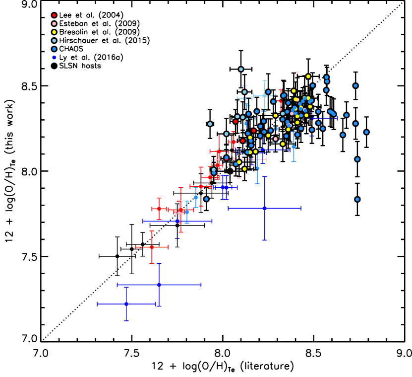
System	Sample	$N_{\textnormal{e}}$	$T_{\textnormal{e}}(\textnormal{{Oii}})$	$T_{\textnormal{e}}(\textnormal{{Nii}})$	$T_{\textnormal{e}}(\textnormal{{Oiii}})$	$\textnormal{O}^{+}/\textnormal{H}^{+}$	$\textnormal{O}^{++}/\textnormal{H}^{+}$	$Z_{\textnormal{Te,direct}}$
		cm-3	K	K	K	$\times 10^{4}$	$\times 10^{4}$
KISSR116	L04	69$\pm 38$	8781$\pm 157$	–	11520$\pm 199$	1.08$\pm 0.27$	0.87$\pm 0.16$	8.29$\pm 0.07$
KISSR286	L04	87$\pm 61$	10729$\pm 367$	–	10460$\pm 450$	0.57$\pm 0.17$	1.15$\pm 0.27$	8.24$\pm 0.08$
KISSB171	L04	69$\pm 23$	10710$\pm 135$	–	11353$\pm 184$	0.50$\pm 0.12$	1.00$\pm 0.18$	8.18$\pm 0.06$
KISSB175	L04	157$\pm 100$	11299$\pm 537$	–	12822$\pm 647$	0.36$\pm 0.12$	0.82$\pm 0.19$	8.07$\pm 0.08$
NGC595	E09	80$\pm 70$	9651$\pm 335$	8896$\pm 457$	7034$\pm 425$	1.11$\pm 0.33$	1.18$\pm 0.39$	8.36$\pm 0.10$
NGC604	E09	86$\pm 70$	13198$\pm 623$	9397$\pm 503$	7590$\pm 284$	0.22$\pm 0.07$	1.95$\pm 0.50$	8.34$\pm 0.10$
NGC1741-C	E09	71$\pm 48$	10912$\pm 296$	10613$\pm 1202$	8066$\pm 642$	0.45$\pm 0.12$	2.17$\pm 0.77$	8.42$\pm 0.13$
VS24	E09	131$\pm 77$	10537$\pm 360$	9034$\pm 462$	7618$\pm 422$	0.53$\pm 0.15$	1.32$\pm 0.38$	8.27$\pm 0.10$
VS38	E09	95$\pm 39$	9383$\pm 174$	8869$\pm 547$	8251$\pm 341$	0.56$\pm 0.14$	0.98$\pm 0.23$	8.19$\pm 0.08$
VS44	E09	126$\pm 75$	13158$\pm 547$	9712$\pm 479$	7771$\pm 280$	0.26$\pm 0.07$	1.61$\pm 0.39$	8.27$\pm 0.09$
J0014-0044-1	G09	87$\pm 39$	15157$\pm 459$	–	12454$\pm 366$	0.09$\pm 0.02$	0.98$\pm 0.19$	8.03$\pm 0.08$
J0202-0047	G09	109$\pm 61$	12679$\pm 423$	–	13686$\pm 608$	0.24$\pm 0.07$	0.60$\pm 0.13$	7.92$\pm 0.08$
J2104-0035-1	G09	112$\pm 59$	14046$\pm 515$	–	19349$\pm 1279$	0.02$\pm 0.01$	0.15$\pm 0.03$	7.24$\pm 0.09$
J2302+0049-1	G09	143$\pm 61$	11739$\pm 352$	–	16338$\pm 694$	0.08$\pm 0.02$	0.44$\pm 0.09$	7.72$\pm 0.08$
J2324-0006	G09	112$\pm 51$	13418$\pm 397$	–	13519$\pm 488$	0.18$\pm 0.05$	0.68$\pm 0.14$	7.93$\pm 0.07$
NGC300-1	B09	253 (lit)	12680$\pm 69$	–	11078$\pm 369$	0.35$\pm 0.09$	0.68$\pm 0.14$	8.01$\pm 0.07$
NGC300-2	B09	182 (lit)	12298$\pm 256$	14256$\pm 1838$	11400$\pm 766$	0.28$\pm 0.09$	1.01$\pm 0.30$	8.11$\pm 0.10$
NGC300-3	B09	20 (lit)	11259$\pm 56$	–	10947$\pm 682$	0.86$\pm 0.21$	0.27$\pm 0.07$	8.05$\pm 0.08$
NGC300-4	B09	25 (lit)	11330$\pm 305$	–	10387$\pm 788$	0.64$\pm 0.23$	0.66$\pm 0.23$	8.11$\pm 0.11$
NGC300-5	B09	20 (lit)	9792$\pm 162$	–	8773$\pm 554$	1.26$\pm 0.40$	1.11$\pm 0.35$	8.37$\pm 0.10$
NGC300-6	B09	20 (lit)	9351$\pm 176$	–	8708$\pm 548$	1.39$\pm 0.47$	1.24$\pm 0.40$	8.42$\pm 0.10$
NGC300-7	B09	247 (lit)	11429$\pm 222$	–	11111$\pm 729$	0.31$\pm 0.10$	2.00$\pm 0.59$	8.37$\pm 0.11$
NGC300-8	B09	20 (lit)	9298$\pm 182$	10001$\pm 960$	9006$\pm 629$	1.49$\pm 0.51$	0.63$\pm 0.21$	8.33$\pm 0.11$
NGC300-9	B09	115 (lit)	10301$\pm 214$	–	8186$\pm 462$	0.63$\pm 0.21$	1.49$\pm 0.48$	8.33$\pm 0.11$
NGC300-10	B09	91 (lit)	8532$\pm 282$	10320$\pm 1214$	8199$\pm 617$	1.23$\pm 0.53$	1.46$\pm 0.60$	8.43$\pm 0.13$
NGC300-11	B09	20 (lit)	11847$\pm 251$	–	9082$\pm 651$	0.58$\pm 0.19$	0.86$\pm 0.29$	8.16$\pm 0.10$
NGC300-14	B09	57 (lit)	10513$\pm 192$	9488$\pm 625$	8397$\pm 438$	0.87$\pm 0.28$	1.06$\pm 0.32$	8.28$\pm 0.10$
NGC300-17	B09	20 (lit)	8096$\pm 132$	9346$\pm 731$	7778$\pm 406$	2.07$\pm 0.70$	1.52$\pm 0.48$	8.55$\pm 0.10$
NGC300-19	B09	20 (lit)	8065$\pm 123$	8888$\pm 655$	8163$\pm 439$	1.87$\pm 0.62$	1.08$\pm 0.34$	8.47$\pm 0.10$
NGC300-20	B09	91 (lit)	8954$\pm 195$	10304$\pm 977$	7842$\pm 456$	0.96$\pm 0.34$	1.72$\pm 0.59$	8.43$\pm 0.11$
NGC300-23	B09	30 (lit)	10227$\pm 209$	8610$\pm 548$	7636$\pm 430$	0.70$\pm 0.24$	1.69$\pm 0.55$	8.38$\pm 0.11$
NGC300-24	B09	88 (lit)	9966$\pm 37$	10121$\pm 451$	8016$\pm 200$	0.86$\pm 0.21$	1.24$\pm 0.25$	8.32$\pm 0.07$
NGC300-26	B09	43 (lit)	11195$\pm 248$	10774$\pm 951$	8612$\pm 499$	0.43$\pm 0.14$	1.33$\pm 0.42$	8.24$\pm 0.11$
NGC300-27	B09	20 (lit)	10159$\pm 184$	10615$\pm 923$	10567$\pm 687$	1.12$\pm 0.37$	0.45$\pm 0.13$	8.20$\pm 0.11$
NGC300-28	B09	20 (lit)	10656$\pm 198$	11508$\pm 1496$	10110$\pm 623$	0.90$\pm 0.29$	0.71$\pm 0.21$	8.21$\pm 0.10$
J1044+0353	I12	141$\pm 44$	15759$\pm 462$	–	19036$\pm 377$	0.02$\pm 0.00$	0.23$\pm 0.04$	7.40$\pm 0.07$
J1132+5722No.1	I12	166$\pm 46$	10887$\pm 232$	–	15048$\pm 580$	0.21$\pm 0.05$	0.20$\pm 0.04$	7.61$\pm 0.07$
J1132+5722No.2	I12	65$\pm 31$	16223$\pm 470$	–	14102$\pm 589$	0.11$\pm 0.03$	0.37$\pm 0.07$	7.69$\pm 0.07$
J1244+3212No.2	I12	125$\pm 42$	9384$\pm 161$	–	13475$\pm 391$	0.61$\pm 0.15$	0.56$\pm 0.11$	8.07$\pm 0.07$
J1244+3212No.3	I12	73$\pm 18$	12899$\pm 152$	–	13493$\pm 185$	0.26$\pm 0.06$	0.40$\pm 0.07$	7.82$\pm 0.06$
J1248+4823	I12	101$\pm 36$	10681$\pm 182$	–	15365$\pm 343$	0.17$\pm 0.04$	0.51$\pm 0.09$	7.83$\pm 0.07$
J1331+4151	I12	94$\pm 27$	11759$\pm 192$	–	16292$\pm 348$	0.10$\pm 0.02$	0.43$\pm 0.08$	7.72$\pm 0.07$
KISSR242	H15	108$\pm 67$	9215$\pm 250$	23730$\pm 2904$	11831$\pm 476$	1.14$\pm 0.33$	0.75$\pm 0.17$	8.28$\pm 0.08$
KISSR451	H15	98$\pm 66$	8606$\pm 250$	–	10803$\pm 501$	2.21$\pm 0.66$	0.70$\pm 0.17$	8.46$\pm 0.10$
KISSR475	H15	116$\pm 71$	7734$\pm 182$	–	10385$\pm 541$	3.37$\pm 0.98$	0.58$\pm 0.14$	8.60$\pm 0.11$
KISSR590	H15	83$\pm 55$	9986$\pm 285$	–	11452$\pm 626$	1.12$\pm 0.32$	0.54$\pm 0.13$	8.22$\pm 0.09$
KISSR653	H15	115$\pm 73$	9075$\pm 258$	–	9862$\pm 606$	1.50$\pm 0.44$	0.59$\pm 0.16$	8.32$\pm 0.10$
KISSR1379	H15	91$\pm 61$	9347$\pm 272$	–	10096$\pm 505$	1.34$\pm 0.39$	0.73$\pm 0.18$	8.32$\pm 0.09$
System	Sample	$N_{\textnormal{e}}$	$T_{\textnormal{e}}(\textnormal{{Oii}})$	$T_{\textnormal{e}}(\textnormal{{Nii}})$	$T_{\textnormal{e}}(\textnormal{{Oiii}})$	$\textnormal{O}^{+}/\textnormal{H}^{+}$	$\textnormal{O}^{++}/\textnormal{H}^{+}$	$Z_{\textnormal{Te,direct}}$
		cm-3	K	K	K	$\times 10^{4}$	$\times 10^{4}$
KISSR1734	H15	136$\pm 76$	11858$\pm 457$	14813$\pm 1453$	12871$\pm 550$	0.31$\pm 0.09$	0.71$\pm 0.16$	8.01$\pm 0.08$
KISSR2117	H15	119$\pm 72$	10736$\pm 361$	11035$\pm 917$	9215$\pm 337$	1.08$\pm 0.32$	1.09$\pm 0.25$	8.34$\pm 0.08$
NGC628+131.9+18.5	CHAOS	302$\pm 140$	12311$\pm 781$	8490$\pm 562$	10233$\pm 552$	0.40$\pm 0.13$	0.28$\pm 0.07$	7.83$\pm 0.09$
NGC628+151.0+22.3	CHAOS	170$\pm 75$	13017$\pm 522$	8597$\pm 650$	8789$\pm 663$	0.35$\pm 0.10$	0.82$\pm 0.26$	8.07$\pm 0.10$
NGC628+232.7+6.6	CHAOS	87$\pm 42$	9868$\pm 211$	–	9829$\pm 1072$	0.91$\pm 0.24$	0.71$\pm 0.27$	8.21$\pm 0.10$
NGC628+237.6+3.0	CHAOS	68$\pm 21$	8966$\pm 96$	–	9642$\pm 1000$	1.66$\pm 0.41$	0.49$\pm 0.18$	8.33$\pm 0.09$
NGC628+289.9-17.4	CHAOS	85$\pm 40$	11822$\pm 290$	–	9832$\pm 355$	0.36$\pm 0.09$	1.39$\pm 0.31$	8.24$\pm 0.08$
NGC628+298.4+12.3	CHAOS	104$\pm 47$	11668$\pm 278$	–	10161$\pm 349$	0.26$\pm 0.07$	1.52$\pm 0.33$	8.25$\pm 0.08$
NGC628+31.6-191.1	CHAOS	92$\pm 79$	11268$\pm 512$	9274$\pm 851$	7926$\pm 492$	0.68$\pm 0.21$	1.10$\pm 0.35$	8.25$\pm 0.10$
NGC628-168.2+150.8	CHAOS	78$\pm 67$	9320$\pm 298$	–	7968$\pm 732$	1.63$\pm 0.49$	1.28$\pm 0.51$	8.46$\pm 0.11$
NGC628-184.7+83.4	CHAOS	99$\pm 60$	9720$\pm 285$	8804$\pm 705$	9056$\pm 476$	1.32$\pm 0.37$	0.58$\pm 0.15$	8.28$\pm 0.09$
NGC628-200.6-4.2	CHAOS	72$\pm 40$	8984$\pm 170$	10220$\pm 1462$	8626$\pm 464$	1.52$\pm 0.41$	0.72$\pm 0.19$	8.35$\pm 0.09$
NGC628-206.5-25.7	CHAOS	97$\pm 49$	9757$\pm 238$	–	7954$\pm 282$	0.89$\pm 0.24$	2.28$\pm 0.53$	8.50$\pm 0.08$
NGC628-42.8-158.2	CHAOS	94$\pm 24$	9576$\pm 114$	9011$\pm 834$	7998$\pm 417$	1.04$\pm 0.25$	1.09$\pm 0.28$	8.33$\pm 0.08$
NGC628-76.2-171.8	CHAOS	78$\pm 49$	9583$\pm 250$	–	9228$\pm 623$	0.97$\pm 0.27$	0.72$\pm 0.21$	8.23$\pm 0.09$
NGC628-90.1+190.2	CHAOS	106$\pm 66$	9730$\pm 271$	9349$\pm 803$	8375$\pm 455$	1.32$\pm 0.37$	0.88$\pm 0.25$	8.34$\pm 0.09$
NGC5457+117.9-235.0	CHAOS	90$\pm 47$	8772$\pm 184$	–	8503$\pm 360$	1.72$\pm 0.45$	0.79$\pm 0.19$	8.40$\pm 0.08$
NGC5457+164.6+9.9	CHAOS	88$\pm 55$	8134$\pm 184$	8299$\pm 297$	7070$\pm 219$	2.12$\pm 0.57$	1.23$\pm 0.28$	8.53$\pm 0.08$
NGC5457+17.3-235.4	CHAOS	80$\pm 75$	10071$\pm 391$	8575$\pm 708$	7836$\pm 386$	0.96$\pm 0.29$	0.95$\pm 0.27$	8.28$\pm 0.09$
NGC5457+189.2-136.3	CHAOS	164$\pm 67$	9519$\pm 248$	9273$\pm 328$	7414$\pm 131$	0.91$\pm 0.24$	2.64$\pm 0.52$	8.55$\pm 0.07$
NGC5457+225.6-124.1	CHAOS	81$\pm 32$	8501$\pm 117$	9274$\pm 503$	8185$\pm 194$	2.00$\pm 0.50$	1.16$\pm 0.24$	8.50$\pm 0.08$
NGC5457+249.3+201.9	CHAOS	99$\pm 41$	10437$\pm 222$	10273$\pm 1254$	8939$\pm 185$	0.89$\pm 0.22$	1.05$\pm 0.21$	8.29$\pm 0.07$
NGC5457+252.2-109.8	CHAOS	75$\pm 42$	8588$\pm 159$	9196$\pm 738$	8676$\pm 252$	1.70$\pm 0.44$	0.86$\pm 0.18$	8.41$\pm 0.08$
NGC5457+254.6-107.2	CHAOS	209$\pm 91$	12035$\pm 522$	9778$\pm 252$	8310$\pm 66$	0.39$\pm 0.11$	2.16$\pm 0.38$	8.41$\pm 0.07$
NGC5457+266.0+534.1	CHAOS	71$\pm 48$	11134$\pm 309$	–	11455$\pm 344$	0.66$\pm 0.17$	0.95$\pm 0.19$	8.21$\pm 0.07$
NGC5457+281.4-71.8	CHAOS	61$\pm 53$	9325$\pm 241$	–	8491$\pm 320$	1.42$\pm 0.40$	0.94$\pm 0.23$	8.37$\pm 0.08$
NGC5457+331.9+401.0	CHAOS	72$\pm 40$	10347$\pm 274$	–	10282$\pm 276$	0.66$\pm 0.17$	1.03$\pm 0.21$	8.23$\pm 0.07$
NGC5457+354.1+71.2	CHAOS	96$\pm 63$	11236$\pm 403$	–	9017$\pm 250$	0.65$\pm 0.18$	1.61$\pm 0.35$	8.35$\pm 0.07$
NGC5457+360.9+75.3	CHAOS	84$\pm 50$	11338$\pm 330$	–	8732$\pm 194$	0.49$\pm 0.13$	1.83$\pm 0.37$	8.36$\pm 0.07$
NGC5457+509.5+264.1	CHAOS	74$\pm 36$	11337$\pm 236$	11765$\pm 1592$	10207$\pm 227$	0.50$\pm 0.13$	1.23$\pm 0.24$	8.24$\pm 0.07$
NGC5457+6.6+886.3	CHAOS	65$\pm 35$	13896$\pm 351$	–	12559$\pm 357$	0.27$\pm 0.07$	0.41$\pm 0.08$	7.84$\pm 0.07$
NGC5457+667.9+174.1	CHAOS	190$\pm 105$	16557$\pm 1144$	12691$\pm 1260$	11959$\pm 409$	0.10$\pm 0.03$	1.19$\pm 0.25$	8.11$\pm 0.08$
NGC5457+67.5+277.0	CHAOS	133$\pm 126$	13902$\pm 1030$	9125$\pm 730$	8021$\pm 320$	0.35$\pm 0.12$	1.88$\pm 0.51$	8.35$\pm 0.10$
NGC5457+692.1+272.9	CHAOS	76$\pm 51$	12906$\pm 438$	–	11441$\pm 349$	0.36$\pm 0.10$	0.74$\pm 0.15$	8.04$\pm 0.07$
NGC5457+96.7+266.9	CHAOS	72$\pm 50$	8878$\pm 204$	9008$\pm 632$	8359$\pm 491$	1.61$\pm 0.43$	0.51$\pm 0.14$	8.33$\pm 0.09$
NGC5457-164.9-333.9	CHAOS	81$\pm 47$	10367$\pm 257$	–	7994$\pm 163$	0.87$\pm 0.23$	1.80$\pm 0.36$	8.43$\pm 0.07$
NGC5457-183.9-179.0	CHAOS	70$\pm 51$	9033$\pm 217$	–	7237$\pm 395$	1.24$\pm 0.33$	1.75$\pm 0.51$	8.47$\pm 0.09$
NGC5457-200.3-193.6	CHAOS	74$\pm 31$	9632$\pm 154$	–	7829$\pm 189$	1.01$\pm 0.24$	1.58$\pm 0.31$	8.41$\pm 0.07$
NGC5457-226.9-366.4	CHAOS	76$\pm 39$	9857$\pm 195$	12445$\pm 1192$	9226$\pm 254$	1.60$\pm 0.41$	0.63$\pm 0.13$	8.35$\pm 0.08$
NGC5457-243.0+159.6	CHAOS	74$\pm 48$	9352$\pm 216$	9442$\pm 553$	7887$\pm 369$	1.51$\pm 0.40$	0.67$\pm 0.17$	8.34$\pm 0.09$
NGC5457-297.7+87.1	CHAOS	96$\pm 69$	10137$\pm 362$	9867$\pm 1094$	8464$\pm 318$	1.14$\pm 0.33$	0.70$\pm 0.17$	8.27$\pm 0.09$
NGC5457-309.4+56.9	CHAOS	74$\pm 44$	8224$\pm 176$	–	8384$\pm 327$	2.10$\pm 0.55$	0.66$\pm 0.15$	8.44$\pm 0.09$
NGC5457-345.5+273.8	CHAOS	94$\pm 81$	16524$\pm 1204$	–	10315$\pm 435$	0.32$\pm 0.10$	1.28$\pm 0.31$	8.20$\pm 0.09$
NGC5457-368.3-285.6	CHAOS	112$\pm 70$	10337$\pm 319$	10346$\pm 512$	8798$\pm 237$	0.84$\pm 0.23$	1.63$\pm 0.35$	8.39$\pm 0.07$
NGC5457-371.1-280.0	CHAOS	90$\pm 51$	10186$\pm 267$	10696$\pm 514$	9270$\pm 225$	0.91$\pm 0.24$	1.11$\pm 0.23$	8.30$\pm 0.07$
NGC5457-377.9-64.9	CHAOS	72$\pm 43$	10129$\pm 229$	9409$\pm 608$	9210$\pm 225$	1.07$\pm 0.28$	0.56$\pm 0.11$	8.21$\pm 0.08$
NGC5457-392.0-270.1	CHAOS	124$\pm 60$	10078$\pm 256$	10704$\pm 461$	9132$\pm 192$	0.60$\pm 0.16$	1.63$\pm 0.32$	8.35$\pm 0.07$
NGC5457-405.5-157.7	CHAOS	70$\pm 37$	8790$\pm 157$	–	10337$\pm 362$	1.79$\pm 0.45$	0.37$\pm 0.08$	8.33$\pm 0.09$
System	Sample	$N_{\textnormal{e}}$	$T_{\textnormal{e}}(\textnormal{{Oii}})$	$T_{\textnormal{e}}(\textnormal{{Nii}})$	$T_{\textnormal{e}}(\textnormal{{Oiii}})$	$\textnormal{O}^{+}/\textnormal{H}^{+}$	$\textnormal{O}^{++}/\textnormal{H}^{+}$	$Z_{\textnormal{Te,direct}}$
		cm-3	K	K	K	$\times 10^{4}$	$\times 10^{4}$
NGC5457-410.3-206.3	CHAOS	68$\pm 39$	8956$\pm 162$	10563$\pm 1047$	8554$\pm 302$	1.96$\pm 0.50$	0.82$\pm 0.18$	8.44$\pm 0.08$
NGC5457-414.1-253.6	CHAOS	81$\pm 38$	9053$\pm 168$	12512$\pm 2099$	9589$\pm 233$	1.07$\pm 0.27$	1.49$\pm 0.30$	8.41$\pm 0.07$
NGC5457-453.8-191.8	CHAOS	71$\pm 30$	9912$\pm 150$	11980$\pm 1463$	10860$\pm 119$	0.93$\pm 0.22$	0.90$\pm 0.16$	8.26$\pm 0.07$
NGC5457-455.7-55.8	CHAOS	54$\pm 22$	9647$\pm 109$	–	10585$\pm 94$	1.11$\pm 0.26$	0.85$\pm 0.15$	8.29$\pm 0.07$
NGC5457-464.7-131.0	CHAOS	57$\pm 30$	11033$\pm 196$	–	11185$\pm 292$	0.68$\pm 0.17$	0.74$\pm 0.14$	8.15$\pm 0.07$
NGC5457-466.1-128.2	CHAOS	68$\pm 31$	10476$\pm 179$	–	11009$\pm 283$	0.93$\pm 0.23$	0.57$\pm 0.11$	8.18$\pm 0.07$
NGC5457-479.7-3.9	CHAOS	74$\pm 40$	9945$\pm 209$	–	11252$\pm 168$	1.08$\pm 0.27$	0.58$\pm 0.10$	8.22$\pm 0.07$
NGC5457-481.4-0.5	CHAOS	88$\pm 49$	10812$\pm 293$	–	12373$\pm 128$	0.75$\pm 0.19$	0.46$\pm 0.08$	8.08$\pm 0.07$
NGC5457-540.5-149.9	CHAOS	58$\pm 20$	11190$\pm 131$	–	13096$\pm 144$	0.41$\pm 0.10$	0.57$\pm 0.10$	7.99$\pm 0.06$
NGC5457-99.6-388.0	CHAOS	183$\pm 69$	11555$\pm 371$	10990$\pm 295$	8992$\pm 70$	0.48$\pm 0.12$	1.80$\pm 0.32$	8.36$\pm 0.06$
PTF12dam	SLSN	93$\pm 30$	13273$\pm 270$	–	13109$\pm 233$	0.22$\pm 0.05$	0.78$\pm 0.14$	8.00$\pm 0.07$

Table 5: Electron densities, temperatures, and oxygen abundances for semi-direct systems from the literature samples.

System	Sample	$N_{\textnormal{e}}$	$T_{\textnormal{e}}(\textnormal{{Oii}})$	$T_{\textnormal{e}}(\textnormal{{Nii}})$	$T_{\textnormal{e}}(\textnormal{{Oiii}})$	$\textnormal{O}^{+}/\textnormal{H}^{+}$	$\textnormal{O}^{++}/\textnormal{H}^{+}$	$Z_{\textnormal{Te,semi-direct}}$
		cm-3	K	K	K	$\times 10^{4}$	$\times 10^{4}$
KISSB23	L04	76$\pm 28$	19389$\pm 1386$	–	14219$\pm 1017$	0.15$\pm 0.02$	0.15$\pm 0.04$	7.78$\pm 0.06$
KISSB61	L04	53$\pm 29$	13502$\pm 316$	–	15108$\pm 353$	0.16$\pm 0.01$	0.42$\pm 0.08$	7.76$\pm 0.06$
KISSB86	L04	61$\pm 22$	10163$\pm 231$	–	11900$\pm 270$	0.71$\pm 0.07$	0.81$\pm 0.15$	8.17$\pm 0.06$
KISSR73	L04	85$\pm 64$	12255$\pm 504$	–	13068$\pm 537$	0.42$\pm 0.07$	0.50$\pm 0.10$	7.96$\pm 0.06$
KISSR85	L04	2093$\pm 1530$	16692$\pm 1658$	–	15283$\pm 1518$	0.08$\pm 0.02$	0.27$\pm 0.07$	7.55$\pm 0.10$
KISSR87	L04	105$\pm 52$	9525$\pm 217$	–	9486$\pm 217$	1.47$\pm 0.18$	1.69$\pm 0.32$	8.41$\pm 0.06$
KISSR310	L04	93$\pm 98$	11665$\pm 1025$	–	14591$\pm 1282$	0.16$\pm 0.06$	0.66$\pm 0.20$	7.91$\pm 0.11$
KISSR311	L04	93$\pm 99$	10174$\pm 825$	–	13189$\pm 1069$	0.74$\pm 0.29$	0.66$\pm 0.20$	8.12$\pm 0.10$
KISSR666	L04	31$\pm 57$	12701$\pm 1244$	–	15814$\pm 1549$	0.02$\pm 0.01$	0.58$\pm 0.18$	7.77$\pm 0.13$
KISSR814	L04	113$\pm 79$	11108$\pm 581$	–	13060$\pm 683$	0.38$\pm 0.09$	0.70$\pm 0.17$	8.03$\pm 0.08$
NGC2363	E09	154$\pm 71$	13339$\pm 323$	15440$\pm 1626$	15400$\pm 373$	0.03$\pm 0.00$	0.54$\pm 0.10$	7.75$\pm 0.08$
NGC4395-70	E09	88$\pm 60$	13780$\pm 907$	–	9998$\pm 658$	0.15$\pm 0.03$	1.02$\pm 0.29$	8.07$\pm 0.11$
NGC4861	E09	116$\pm 71$	11106$\pm 519$	14082$\pm 2501$	12302$\pm 575$	0.19$\pm 0.04$	0.99$\pm 0.23$	8.07$\pm 0.09$
NGC5461	E09	224$\pm 196$	9022$\pm 443$	9928$\pm 704$	7945$\pm 390$	0.60$\pm 0.16$	2.33$\pm 0.69$	8.47$\pm 0.11$
J0301-0059-1	G09	72$\pm 42$	13044$\pm 854$	–	11972$\pm 784$	0.48$\pm 0.12$	0.48$\pm 0.12$	8.14$\pm 0.08$
J0301-0059-2	G09	70$\pm 42$	14028$\pm 1495$	–	13386$\pm 1427$	0.34$\pm 0.11$	0.34$\pm 0.11$	7.97$\pm 0.10$
J0338+0013	G09	127$\pm 62$	13871$\pm 778$	–	17071$\pm 957$	0.05$\pm 0.01$	0.37$\pm 0.08$	7.63$\pm 0.09$
G0405-3648-1	G09	41$\pm 23$	19294$\pm 1710$	–	14440$\pm 1280$	0.08$\pm 0.01$	0.22$\pm 0.05$	7.47$\pm 0.09$
G0405-3648-2	G09	124$\pm 31$	19859$\pm 1026$	–	17629$\pm 911$	0.08$\pm 0.01$	0.09$\pm 0.02$	7.37$\pm 0.05$
G0405-3648-3	G09	53$\pm 23$	18797$\pm 1425$	–	20486$\pm 1553$	0.06$\pm 0.01$	0.06$\pm 0.01$	7.24$\pm 0.06$
J0519+0007	G09	367$\pm 161$	15396$\pm 1126$	23742$\pm 3423$	19272$\pm 1409$	0.02$\pm 0.00$	0.24$\pm 0.05$	7.40$\pm 0.09$
J2104-0035-3+4	G09	22$\pm 20$	24512$\pm 3360$	–	19261$\pm 2640$	0.03$\pm 0.01$	0.04$\pm 0.01$	7.02$\pm 0.09$
J2302+0049-2	G09	60$\pm 32$	15311$\pm 861$	–	14442$\pm 812$	0.16$\pm 0.03$	0.33$\pm 0.07$	7.69$\pm 0.07$
DDO68No.2	I12	15$\pm 18$	23799$\pm 1515$	–	16560$\pm 1054$	0.02$\pm 0.00$	0.10$\pm 0.02$	7.08$\pm 0.08$
DDO68No.3a	I12	71$\pm 54$	26779$\pm 3372$	–	16448$\pm 2071$	0.02$\pm 0.00$	0.07$\pm 0.02$	6.95$\pm 0.10$
J0113+0052No.1	I12	–	18436$\pm 2701$	–	22135$\pm 3243$	0.04$\pm 0.01$	0.07$\pm 0.02$	7.04$\pm 0.09$
J0113+0052No.3	I12	–	14006$\pm 2190$	–	25844$\pm 4042$	0.09$\pm 0.04$	0.06$\pm 0.02$	7.19$\pm 0.09$
J0851+8416	I12	36$\pm 27$	16599$\pm 1298$	–	14430$\pm 1129$	0.09$\pm 0.02$	0.33$\pm 0.08$	7.61$\pm 0.09$
J0906+2528No.2	I12	14$\pm 22$	18365$\pm 2235$	–	16485$\pm 2007$	0.07$\pm 0.02$	0.17$\pm 0.05$	7.38$\pm 0.10$
J0908+0517No.2	I12	86$\pm 29$	15147$\pm 507$	–	15466$\pm 517$	0.07$\pm 0.01$	0.36$\pm 0.07$	7.64$\pm 0.07$
J1016+3754	I12	120$\pm 39$	14599$\pm 199$	–	16630$\pm 227$	0.05$\pm 0.00$	0.35$\pm 0.06$	7.60$\pm 0.07$
J1016+5823No.1	I12	57$\pm 20$	14662$\pm 206$	–	14596$\pm 206$	0.10$\pm 0.00$	0.42$\pm 0.07$	7.72$\pm 0.06$
J1016+5823No.2	I12	46$\pm 30$	18221$\pm 1490$	–	14616$\pm 1195$	0.09$\pm 0.02$	0.24$\pm 0.06$	7.51$\pm 0.09$
J1016+5823No.3	I12	25$\pm 17$	15055$\pm 248$	–	16179$\pm 267$	0.08$\pm 0.00$	0.32$\pm 0.06$	7.60$\pm 0.06$
J1056+3608No.1	I12	675$\pm 488$	18824$\pm 2334$	–	21494$\pm 2665$	0.03$\pm 0.01$	0.09$\pm 0.02$	7.05$\pm 0.09$
J1056+3608No.2	I12	15$\pm 24$	13358$\pm 3762$	–	25760$\pm 7255$	0.14$\pm 0.11$	0.04$\pm 0.02$	7.48$\pm 0.15$
J1056+3608No.3	I12	25$\pm 31$	18067$\pm 3111$	–	19860$\pm 3420$	0.07$\pm 0.03$	0.08$\pm 0.03$	7.27$\pm 0.10$
J1119+0935No.2	I12	74$\pm 31$	17828$\pm 1253$	–	13505$\pm 949$	0.11$\pm 0.02$	0.29$\pm 0.07$	7.61$\pm 0.08$
J1119+5130	I12	166$\pm 75$	17683$\pm 511$	–	16492$\pm 476$	0.06$\pm 0.00$	0.20$\pm 0.04$	7.42$\pm 0.06$
J1132+5722No.3	I12	30$\pm 34$	14000$\pm 1007$	–	16141$\pm 1160$	0.14$\pm 0.03$	0.33$\pm 0.07$	7.67$\pm 0.08$
J1154+4636	I12	134$\pm 40$	14705$\pm 380$	–	14671$\pm 379$	0.13$\pm 0.01$	0.38$\pm 0.07$	7.71$\pm 0.06$
J1215+5223	I12	73$\pm 37$	17772$\pm 600$	–	15775$\pm 533$	0.07$\pm 0.01$	0.22$\pm 0.04$	7.46$\pm 0.07$
J1224+3724	I12	80$\pm 27$	12861$\pm 288$	–	15635$\pm 350$	0.11$\pm 0.01$	0.48$\pm 0.09$	7.77$\pm 0.07$
J1226-0115No.1	I12	50$\pm 16$	12912$\pm 239$	–	15389$\pm 284$	0.11$\pm 0.01$	0.50$\pm 0.09$	7.78$\pm 0.07$
J1226-0115No.2	I12	128$\pm 37$	13453$\pm 372$	–	14691$\pm 406$	0.10$\pm 0.01$	0.51$\pm 0.10$	7.79$\pm 0.07$
J1235+2755No.1	I12	77$\pm 39$	13001$\pm 1535$	–	22649$\pm 2675$	0.17$\pm 0.06$	0.09$\pm 0.02$	7.50$\pm 0.07$
J1235+2755No.2	I12	62$\pm 18$	14606$\pm 389$	–	13319$\pm 355$	0.19$\pm 0.01$	0.44$\pm 0.08$	7.80$\pm 0.06$
J1235+2755No.3	I12	64$\pm 24$	13373$\pm 564$	–	14864$\pm 627$	0.27$\pm 0.04$	0.34$\pm 0.07$	7.78$\pm 0.06$
System	Sample	$N_{\textnormal{e}}$	$T_{\textnormal{e}}(\textnormal{{Oii}})$	$T_{\textnormal{e}}(\textnormal{{Nii}})$	$T_{\textnormal{e}}(\textnormal{{Oiii}})$	$\textnormal{O}^{+}/\textnormal{H}^{+}$	$\textnormal{O}^{++}/\textnormal{H}^{+}$	$Z_{\textnormal{Te,semi-direct}}$
		cm-3	K	K	K	$\times 10^{4}$	$\times 10^{4}$
J1241-0340	I12	84$\pm 28$	12977$\pm 373$	–	15998$\pm 459$	0.15$\pm 0.02$	0.41$\pm 0.08$	7.74$\pm 0.06$
J1244+3212No.1	I12	96$\pm 21$	13925$\pm 199$	–	14073$\pm 201$	0.21$\pm 0.01$	0.41$\pm 0.07$	7.79$\pm 0.06$
J1257+3341No.1	I12	119$\pm 71$	20481$\pm 2922$	–	15367$\pm 2193$	0.08$\pm 0.02$	0.14$\pm 0.05$	7.43$\pm 0.10$
J1257+3341No.3	I12	250$\pm 133$	19337$\pm 2485$	–	16135$\pm 2073$	0.10$\pm 0.03$	0.13$\pm 0.04$	7.50$\pm 0.09$
J1327+4022	I12	95$\pm 42$	13976$\pm 202$	–	16356$\pm 236$	0.05$\pm 0.00$	0.41$\pm 0.07$	7.66$\pm 0.07$
J1355+4651	I12	–	13586$\pm 218$	–	18911$\pm 304$	0.02$\pm 0.00$	0.33$\pm 0.06$	7.55$\pm 0.07$
J1403+5804No.2	I12	89$\pm 58$	16176$\pm 1246$	–	19336$\pm 1489$	0.07$\pm 0.01$	0.15$\pm 0.03$	7.35$\pm 0.07$
J1608+3528	I12	773$\pm 594$	11876$\pm 422$	–	17369$\pm 618$	0.04$\pm 0.01$	0.52$\pm 0.10$	7.75$\pm 0.08$
PHL293B	I12	49$\pm 21$	13923$\pm 400$	–	16456$\pm 473$	0.10$\pm 0.01$	0.35$\pm 0.06$	7.66$\pm 0.07$
SBS1420+544	I12	68$\pm 27$	12371$\pm 207$	–	16066$\pm 269$	0.08$\pm 0.00$	0.53$\pm 0.09$	7.78$\pm 0.07$
UGC521A	B12	38$\pm 48$	14333$\pm 911$	–	16611$\pm 1056$	0.15$\pm 0.03$	0.27$\pm 0.06$	7.62$\pm 0.07$
UGC695E	B12	36$\pm 29$	16264$\pm 3649$	–	15909$\pm 3569$	0.22$\pm 0.12$	0.13$\pm 0.06$	7.85$\pm 0.14$
UGC1056A	B12	139$\pm 142$	14878$\pm 3407$	–	13312$\pm 3048$	0.31$\pm 0.20$	0.31$\pm 0.17$	7.98$\pm 0.17$
UGC1056B	B12	46$\pm 56$	12719$\pm 2906$	–	11594$\pm 2649$	0.41$\pm 0.30$	0.64$\pm 0.40$	8.03$\pm 0.21$
UGC1176A	B12	78$\pm 92$	13152$\pm 2154$	–	12237$\pm 2004$	0.30$\pm 0.15$	0.60$\pm 0.27$	7.95$\pm 0.16$
NGC784A	B12	104$\pm 126$	11733$\pm 1869$	–	11435$\pm 1821$	0.37$\pm 0.23$	0.85$\pm 0.43$	8.09$\pm 0.18$
NGC784B	B12	85$\pm 137$	13632$\pm 4175$	–	12317$\pm 3772$	0.28$\pm 0.27$	0.55$\pm 0.45$	7.92$\pm 0.28$
UGC2716A	B12	73$\pm 73$	12012$\pm 2157$	–	12335$\pm 2214$	0.35$\pm 0.22$	0.69$\pm 0.35$	8.02$\pm 0.18$
NGC2537A	B12	114$\pm 147$	12291$\pm 2321$	–	8859$\pm 1673$	0.64$\pm 0.42$	1.06$\pm 0.73$	8.42$\pm 0.23$
NGC2537B	B12	79$\pm 71$	17340$\pm 3522$	–	10359$\pm 2104$	0.23$\pm 0.12$	0.50$\pm 0.31$	8.07$\pm 0.21$
UGC4278B	B12	90$\pm 77$	18670$\pm 1872$	–	13611$\pm 1365$	0.13$\pm 0.03$	0.23$\pm 0.07$	7.67$\pm 0.09$
UGC4278A	B12	101$\pm 89$	17432$\pm 2122$	–	13548$\pm 1649$	0.11$\pm 0.04$	0.32$\pm 0.11$	7.63$\pm 0.12$
NGC2552A	B12	101$\pm 64$	12281$\pm 940$	–	9807$\pm 751$	0.47$\pm 0.13$	0.98$\pm 0.30$	8.18$\pm 0.11$
UGC4393B	B12	60$\pm 64$	12443$\pm 2439$	–	10897$\pm 2136$	0.42$\pm 0.27$	0.78$\pm 0.45$	8.08$\pm 0.20$
UGC4393C	B12	87$\pm 94$	12208$\pm 2067$	–	12054$\pm 2040$	0.61$\pm 0.36$	0.45$\pm 0.22$	8.23$\pm 0.15$
CGCG035-007A	B12	57$\pm 38$	11938$\pm 3789$	–	17590$\pm 5582$	0.61$\pm 0.69$	0.13$\pm 0.08$	8.11$\pm 0.18$
UGC5139A	B12	59$\pm 47$	13631$\pm 1227$	–	12438$\pm 1119$	0.24$\pm 0.07$	0.58$\pm 0.17$	7.91$\pm 0.10$
IC559A	B12	48$\pm 75$	12998$\pm 3296$	–	10715$\pm 2717$	0.45$\pm 0.35$	0.71$\pm 0.52$	8.15$\pm 0.24$
UGC5272A	B12	71$\pm 38$	13067$\pm 495$	–	13411$\pm 508$	0.14$\pm 0.02$	0.63$\pm 0.13$	7.89$\pm 0.08$
UGC5340A	B12	522$\pm 473$	20359$\pm 2088$	–	18830$\pm 1932$	0.02$\pm 0.01$	0.11$\pm 0.03$	7.12$\pm 0.09$
UGC5423A	B12	80$\pm 64$	14273$\pm 1239$	–	14345$\pm 1246$	0.20$\pm 0.06$	0.37$\pm 0.11$	7.76$\pm 0.10$
UGC5423B	B12	88$\pm 102$	14339$\pm 2467$	–	13841$\pm 2381$	0.17$\pm 0.09$	0.44$\pm 0.19$	7.78$\pm 0.15$
UGC5797A	B12	62$\pm 56$	11104$\pm 1727$	–	13132$\pm 2042$	0.32$\pm 0.18$	0.75$\pm 0.30$	8.03$\pm 0.15$
UGC5923A	B12	81$\pm 136$	13516$\pm 5481$	–	14840$\pm 6018$	0.35$\pm 0.43$	0.25$\pm 0.22$	7.95$\pm 0.27$
NGC3741A	B12	89$\pm 42$	16527$\pm 1931$	–	14874$\pm 1738$	0.11$\pm 0.03$	0.28$\pm 0.08$	7.59$\pm 0.10$
NGC3738A	B12	87$\pm 44$	12707$\pm 1053$	–	11187$\pm 927$	0.48$\pm 0.13$	0.64$\pm 0.18$	8.14$\pm 0.09$
NGC3738B	B12	92$\pm 71$	11353$\pm 2004$	–	11854$\pm 2092$	0.72$\pm 0.45$	0.57$\pm 0.28$	8.20$\pm 0.16$
UGC6817A	B12	89$\pm 46$	17457$\pm 772$	–	15767$\pm 698$	0.06$\pm 0.01$	0.24$\pm 0.05$	7.48$\pm 0.08$
NGC4163A	B12	48$\pm 48$	18162$\pm 3095$	–	17072$\pm 2909$	0.19$\pm 0.08$	0.04$\pm 0.01$	8.11$\pm 0.09$
CGCG269-049C	B12	–	18852$\pm 4262$	–	18508$\pm 4184$	0.08$\pm 0.04$	0.09$\pm 0.04$	7.35$\pm 0.14$
CGCG269-049A	B12	87$\pm 49$	18265$\pm 983$	–	16115$\pm 867$	0.06$\pm 0.01$	0.20$\pm 0.04$	7.41$\pm 0.08$
UGC7577A	B12	114$\pm 65$	11028$\pm 673$	–	12829$\pm 782$	0.36$\pm 0.08$	0.77$\pm 0.17$	8.05$\pm 0.08$
NGC4449C	B12	84$\pm 54$	13373$\pm 1525$	–	9995$\pm 1140$	0.50$\pm 0.18$	0.74$\pm 0.29$	8.29$\pm 0.13$
NGC4449B	B12	84$\pm 72$	12439$\pm 1312$	–	9662$\pm 1019$	0.56$\pm 0.20$	0.91$\pm 0.35$	8.29$\pm 0.13$
NGC4449A	B12	90$\pm 74$	9398$\pm 296$	–	9046$\pm 285$	1.83$\pm 0.33$	1.56$\pm 0.34$	8.44$\pm 0.07$
UGC7605A	B12	25$\pm 32$	17452$\pm 2378$	–	13604$\pm 1853$	0.14$\pm 0.04$	0.28$\pm 0.10$	7.65$\pm 0.12$
NGC4656A	B12	17$\pm 70$	10127$\pm 1205$	–	11885$\pm 1414$	0.22$\pm 0.11$	1.23$\pm 0.46$	8.16$\pm 0.15$
UGC8201A	B12	74$\pm 117$	16203$\pm 2326$	–	13343$\pm 1915$	0.13$\pm 0.05$	0.38$\pm 0.14$	7.71$\pm 0.13$
System	Sample	$N_{\textnormal{e}}$	$T_{\textnormal{e}}(\textnormal{{Oii}})$	$T_{\textnormal{e}}(\textnormal{{Nii}})$	$T_{\textnormal{e}}(\textnormal{{Oiii}})$	$\textnormal{O}^{+}/\textnormal{H}^{+}$	$\textnormal{O}^{++}/\textnormal{H}^{+}$	$Z_{\textnormal{Te,semi-direct}}$
		cm-3	K	K	K	$\times 10^{4}$	$\times 10^{4}$
UGC8508A	B12	53$\pm 69$	15753$\pm 1668$	–	13963$\pm 1479$	0.12$\pm 0.03$	0.37$\pm 0.11$	7.69$\pm 0.10$
UGC8638A	B12	84$\pm 67$	12586$\pm 286$	–	12276$\pm 279$	0.29$\pm 0.02$	0.68$\pm 0.12$	7.98$\pm 0.06$
UGC8638B	B12	189$\pm 260$	12970$\pm 1915$	–	12315$\pm 1818$	0.23$\pm 0.11$	0.68$\pm 0.28$	7.96$\pm 0.15$
UGC8837A	B12	84$\pm 43$	18654$\pm 1582$	–	12841$\pm 1089$	0.23$\pm 0.05$	0.18$\pm 0.05$	8.05$\pm 0.07$
NGC5477A	B12	111$\pm 64$	12431$\pm 1199$	–	12025$\pm 1160$	0.21$\pm 0.07$	0.81$\pm 0.25$	8.01$\pm 0.12$
KISSR148	H15	70$\pm 47$	11158$\pm 711$	–	9586$\pm 611$	1.01$\pm 0.27$	0.94$\pm 0.26$	8.44$\pm 0.09$
KISSR258	H15	168$\pm 98$	12073$\pm 1375$	–	22508$\pm 2564$	0.34$\pm 0.14$	0.05$\pm 0.01$	7.92$\pm 0.08$
KISSR1056	H15	106$\pm 67$	11138$\pm 488$	–	10494$\pm 460$	0.89$\pm 0.18$	0.82$\pm 0.19$	8.31$\pm 0.08$
KISSR2132	H15	90$\pm 58$	11316$\pm 606$	–	10993$\pm 589$	1.25$\pm 0.30$	0.64$\pm 0.16$	8.43$\pm 0.07$
NGC628+252.1-92.1	CHAOS	88$\pm 46$	15262$\pm 1176$	13829$\pm 2034$	11489$\pm 885$	0.29$\pm 0.06$	0.48$\pm 0.13$	8.02$\pm 0.09$
NGC628+254.3-42.8	CHAOS	72$\pm 38$	16125$\pm 1296$	–	11291$\pm 907$	0.32$\pm 0.08$	0.40$\pm 0.11$	8.14$\pm 0.09$
NGC628+261.9-99.7	CHAOS	56$\pm 65$	14681$\pm 1569$	–	10713$\pm 1145$	0.45$\pm 0.15$	0.49$\pm 0.19$	8.28$\pm 0.12$
NGC5457+1.0+885.8	CHAOS	66$\pm 37$	18157$\pm 519$	–	12624$\pm 361$	0.17$\pm 0.02$	0.28$\pm 0.05$	7.85$\pm 0.06$
NGC5457+324.5+415.8	CHAOS	74$\pm 38$	12078$\pm 264$	–	10563$\pm 231$	0.65$\pm 0.05$	0.70$\pm 0.13$	8.29$\pm 0.06$
NGC5457-397.4-71.7	CHAOS	63$\pm 26$	15334$\pm 712$	–	9011$\pm 418$	0.31$\pm 0.04$	0.85$\pm 0.20$	8.25$\pm 0.08$
NGC5457-8.5+886.7	CHAOS	40$\pm 30$	19612$\pm 729$	–	12505$\pm 465$	0.13$\pm 0.01$	0.26$\pm 0.05$	7.76$\pm 0.07$
MMT10	L16	113$\pm 77$	12373$\pm 534$	–	13873$\pm 598$	0.21$\pm 0.03$	0.59$\pm 0.12$	7.90$\pm 0.07$
MMT11	L16	1147$\pm 504$	10133$\pm 555$	–	13209$\pm 724$	0.71$\pm 0.16$	0.63$\pm 0.14$	8.11$\pm 0.07$
MMT15	L16	114$\pm 83$	11004$\pm 1870$	–	22255$\pm 3782$	0.37$\pm 0.24$	0.11$\pm 0.03$	7.71$\pm 0.10$
MMT16	L16	279$\pm 363$	13513$\pm 2909$	–	23462$\pm 5051$	0.10$\pm 0.06$	0.12$\pm 0.04$	7.33$\pm 0.12$
MMT18	L16	53$\pm 38$	15317$\pm 2511$	–	22886$\pm 3752$	0.07$\pm 0.03$	0.10$\pm 0.03$	7.22$\pm 0.10$
MMT19	L16	–	12045$\pm 507$	–	14206$\pm 598$	0.19$\pm 0.03$	0.61$\pm 0.12$	7.91$\pm 0.07$
MMT26	L16	53$\pm 27$	12121$\pm 1259$	–	14574$\pm 1514$	0.56$\pm 0.20$	0.25$\pm 0.07$	8.12$\pm 0.08$
MMT28	L16	–	11241$\pm 2668$	–	17746$\pm 4211$	0.23$\pm 0.21$	0.37$\pm 0.19$	7.78$\pm 0.19$
MMT32	L16	121$\pm 73$	9724$\pm 798$	–	10349$\pm 850$	1.05$\pm 0.38$	1.19$\pm 0.36$	8.31$\pm 0.10$
SN2010kd	SLSN	–	13352$\pm 2792$	–	19336$\pm 4043$	0.09$\pm 0.06$	0.26$\pm 0.10$	7.54$\pm 0.14$
SN2011ke	SLSN	–	14672$\pm 647$	–	17091$\pm 754$	0.08$\pm 0.01$	0.29$\pm 0.06$	7.57$\pm 0.07$
LSQ14an	SLSN	102$\pm 76$	10477$\pm 865$	–	13310$\pm 1099$	0.88$\pm 0.31$	0.67$\pm 0.18$	8.12$\pm 0.09$
PTF10bfz	SLSN	22$\pm 56$	13730$\pm 2157$	–	16231$\pm 2549$	0.16$\pm 0.08$	0.32$\pm 0.12$	7.68$\pm 0.13$
SN2012il	SLSN	151$\pm 125$	12020$\pm 940$	–	13802$\pm 1080$	0.25$\pm 0.07$	0.60$\pm 0.15$	7.93$\pm 0.09$
PTF09as	SLSN	45$\pm 62$	11755$\pm 1508$	–	15227$\pm 1953$	0.25$\pm 0.11$	0.49$\pm 0.16$	7.87$\pm 0.11$
SN2010gx	SLSN	168$\pm 236$	13560$\pm 1876$	–	19868$\pm 2749$	0.09$\pm 0.04$	0.22$\pm 0.07$	7.50$\pm 0.11$
GAIA16apd	SLSN	36$\pm 67$	13235$\pm 1174$	–	13572$\pm 1204$	0.14$\pm 0.04$	0.60$\pm 0.18$	7.87$\pm 0.11$

Appendix D Linear fitting methods

We adopt two distinct methods when making linear fits to the three key relations discussed in this work, namely, the $Z_{\textnormal{Te}}$ – $a$ relation (Eqn. 5.1), our $[\textnormal{{Oiii}}]$/$[\textnormal{{Oii}}]$-based semi-direct $Z_{\textnormal{Te}}$ correction (Eqn. 14), and the galaxy MZR (Eqn. 6). An overview of these two fitting methods is provided below.

D.1 Least-squares fitting

The first method we adopt is the linear least-squares approximation provided by the IDL routine MPFITEXY (Williams et al. 2010), which depends on the MPFIT package (Markwardt 2009). This routine utilises the $\chi^{2}$ minimisation technique to obtain a straight-line best fit to the data, accounting for errors in both the ordinate and abscissa axes and a determination of the intrinsic scatter which is adjusted to ensure the reduced $\chi^{2}\sim{}1$ using the method outlined in Bedregal et al. (2006).

D.2 Nested Sampling fitting

In addition to the linear least-squares fitting method outlined above, we also applied a simple Bayesian fit using nested sampling. For this we used the dynesty package (Speagle 2019). For deriving the posterior we used dynamic nested sampling (Higson et al. 2017).

D.2.1 Linear models

For the comparison between the $Z_{\textnormal{Te}}$ – $a$ relation and the $Z_{\textnormal{Te}}$ – $T_{\textnormal{e}}(\textnormal{{Oiii}})$ and $Z_{\textnormal{Te}}$ – $T_{\textnormal{e}}(\textnormal{{Oii}})$ relations (§5.1), we use the same prior in all cases. We note that the derived evidence depends very strongly on the prior, and that improper priors can lead to inaccurate results.

In general, each relation combines one or more observable $X$ with the desired quantity $Z$, such that for each observable we have a dataset of $X_{i}$ and $Z_{i}$.

We assume that each measurement, $X_{i,\text{obs}}$, is drawn from a normal distribution centered at the value of the model function, $f_{x}$, for this measurement pair with an effective standard deviation value. This gives,

$$Z_{i,\text{obs}}\sim\mathcal{N}(f_{x}(X_{i,\text{obs}},\theta),\sigma_{Z,i,\text{eff}})$$ (24)

The effective standard deviation $\sigma_{Z,i,\text{eff}}$ is defined as follows and includes the standard deviation of both observables as well as an additional scattering term $f$,

$$\sigma_{Z,i,\text{eff}}=\sqrt{\sigma_{Z,i,\text{obs}}^{2}+\left(\frac{\partial f_{x}(X_{i,\text{true}},\theta)}{\partial X_{i,\text{true}}}\right)^{2}\sigma_{X,i,\text{obs}}^{2}+f_{x}(X_{i,\text{obs}},\theta)^{2}\,f^{2}}$$ (25)

Where $X_{i,\text{true}}$ is the true value of $X_{i}$, which $X_{i,\text{obs}}$ is sampled from (conceptually). Since sampling an $N+3$ dimensional cube is quite expensive, we approximated the partial derivative using the observed value. Since the range for values for $Z$ are typically quite small, other errors (systematic uncertainties, for instance) will dominate over the approximation error. In the case where $\partial f_{x}/\partial X_{i,\text{true}}$ does not depend on $X_{i,\text{true}}$, the solution is exact (as is the case for the simple linear relations).

For most cases in the paper we use the following model function:

$$f_{x}(X,\theta\{\alpha,\beta\})=\alpha X+\beta$$ (26)

This is used for the various temperature – metallicity fits, as well as the MZR fit. We use weak uninformative priors for the parameters:

$$\ln\alpha^{-1} \sim\mathcal{N}(-8,10)$$ (27)

$$\beta \sim\mathcal{N}(0,1000)$$ (28)

$$\ln f \sim\mathcal{U}(-21,1)$$ (29)

When using the information from the posterior, one has to keep in mind the whole covariance matrix,

$$\mathbb{C_{\alpha,\beta}}=\left(\begin{array}[]{ll}\sigma_{\alpha}^{2}&\sigma_{\alpha}\sigma_{\beta}\rho\\ \sigma_{\alpha}\sigma_{\beta}\rho&\sigma_{\beta}^{2}\end{array}\right)$$ (30)

While the off-axis elements between most parameters are mostly zero, the slope $\alpha$ and intercept $\beta$ are highly correlated.

D.2.2 $Z_{\textnormal{Te}}$ correction factor

To fit the semi-direct $Z_{\textnormal{Te}}$ correction factor discussed in §5.3, we used a fairly simple linear model that assumes all measurements below a certain critical $[\textnormal{{Oiii}}]$/$[\textnormal{{Oii}}]$ ratio, $x_{c}\sim\mathcal{U}(-0.5,1.0)\ [\text{dex}]$, under-estimate the metallicity by a $[\textnormal{{Oiii}}]$/$[\textnormal{{Oii}}]$-dependent factor. The location of the cutoff $x_{c}$ was left as a free parameter with a non-informative prior.

We assumed the following relation for this correction factor:

$$f_{\text{cor}}(x,\theta\{\alpha,x_{c}\})=\bigg{\{}\begin{array}[]{ll}\alpha\,(x-x_{c})&\text{for}\,x\leq x_{c}\\ 0&\text{for}\,x>x_{c}\;\;\;,\end{array}$$ (31)

which is equivalent to Eqn. 14.