The Distance Measurements of Supernova Remnants in The Fourth Galactic Quadrant ^∗

Abstract

We take advantage of the red clump stars to build the relation of the optical extinction ($\rm A_{V}$) and distance in each direction of supernova remnants (SNRs) with known extinction in the fourth Galactic quadrant. The distances of 9 SNRs are well determined by this method. Their uncertainties range from 10% to 30%, which is significantly improved for 8 SNRs, G279.0+1.1, G284.3-1.8, G296.1-0.5, G299.2-2.9, G308.4-1.4, G309.2-0.6, G309.8-2.6, G332.4-0.4. In addition, SNR G284.3-1.8 with the new distance of 5.5 kpc is not likely associated with the PSR J1016-5857 at 3 kpc.

1 Introduction

Distance is a basic and important parameter for a supernova remnant (SNR) to constrain its size, age, expansion velocity and the explosion energy of the progenitor supernova (e.g., Tian & Leahy 2008; Zhou et al. 2018). However, it is challenging to obtain reliable distances of supernova remnants. About 30% of SNRs’ distances are available in the Galactic SNRs’ catalog of Green (2014) and $\sim$ 50% of SNRs have distances in the catalogue of Ferrand & Safi-Harb (2012). Most of these distances are not given the uncertainty estimates.

There are several methods to measure the distance of SNRs. Firstly, the kinematic distances of SNRs are likely to be measured based on their HI absorptions or molecular line emissions from the clouds interacting with them (e.g., Leahy & Tian 2010; Su et al. 2011; Ranasinghe & Leahy 2018). Secondly, for shell-type radio SNRs, distances can be estimated by the $\Sigma$-D relation (e.g., Case & Bhattacharya 1998). Thirdly, the distances of SNRs are usually equivalent to the distances of their possible associations, for examples, OB associations (e.g. Cha et al. 1999, Vela remnant), pulsars (e.g. Cordes & Lazio 2002). For some rare SNRs, distances can also be obtained by proper motion (e.g. Vink 2008; Katsuda et al. 2008, Kepler’s supernova remnant), Sedov estimates (Bocchino et al. 2000), blast wave method (McKee & Cowie 1975), or extinction measurement (Chen et al. 2017; Zhao et al. 2018).

Red clump (RC) stars are characterized by concentrating in an obvious region of the colour-magnitude diagrams (CMDs) (Gao et al. 2009). They are usually low mass stars in the early stage of core-He burning and widely used to trace distances, and probe extinction towards Galactic objects since the dispersion of their absolute magnitude and the intrinsic colour are small (Girardi 2016). The relation of extinction and distance has been used to estimate the distances of the objects with known extinction, such as pulsars (Durant & van Kerkwijk 2006), Low-mass X-ray binaries (Güver et al. 2010). Zhu et al. (2015) first applied the RC method to determine the distance of SNR G332.5-5.6. Shan et al. (2018) applied the similar method to systematically analyse the extinction distances towards SNRs in the first Galactic quadrant and independently obtained new extinction distances of 15 SNRs. Their results have proved that the distances traced by RC stars are reliable and consistent with the kinematic distances. This paper presents our new results aiming at the SNRs in the rest of Galactic quadrants.

2 Method

We follow the RC method of Shan et al. (2018). Here we briefly describe this method. To select the RC stars, we build the Ks (hereafter K) vs. J-K CMD in the direction of each SNR with the 2MASS All-Sky Point Source Catalogue (Skrutskie et al. 2006). The area around the SNR is $1^{\circ}$ $\times$ $0.5^{\circ}$ ($\bigtriangleup l\,$ $\times$ $\bigtriangleup b\,$). Fig. 1 (a) shows an example of SNR 308.2-1.4.

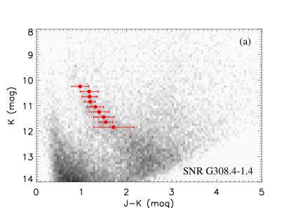
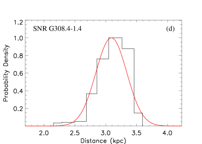
Figure 1: (a) The CMD in the direction of G308.4-1.4 within 0.5 deg², the red dot and lines show the fitted location of the RC peak density and its extent with $1\sigma$. (b) Histogram of the $\rm J-K$ values of the selected stars in the $\rm 10.6<K<11.1$. The black curve is the best fit to this histogram. The red dotted curves are the Gaussian and power-law components, respectively. (c) The $\rm A_{V}$-D relation in the direction of G308.4-1.4. The dashed line is $\rm A_{v}$ value of this SNR. The dotted lines are the uncertainties of $\rm A_{v}$. (d) Probability distribution over distance to the SNRs and the best-fit Gaussian model.

We bin the stars sample into a number of horizontal strips according to K magnitude. The sample of each bin is constructed as the stars count histogram. Then we use the function below to fit the histogram (Durant & van Kerkwijk 2006):

$$\rm N=A_{RCs}exp\{\frac{-[(J-K)-(J-K)_{peak}]^{2}}{2\sigma^{2}}\}+A_{C}(J-K)^{\alpha}$$ (1)

Here ($\rm J-K$) represents the stellar colour, $\rm A_{RCs}$, and $\rm A_{C}$ stand for the normalizations of RC stars and contaminant stars, respectively. The first term of this function is a Gaussian function to fit the RC stars distribution; the second term is a power law to fit the contaminant stars (see Fig. 1 (b)). The best fit yields the stellar colour of RC stars at peak density $(J-K)_{\rm peak}$ for each strip. The extinction and distance are calculated from

$$\rm A_{K}=0.67\times[(J-K)_{peak}-(J-K)_{0}]$$ (2)

$$\rm\frac{A_{K}}{A_{V}}=0.1615-\frac{0.1483}{R_{V}}$$ (3)

$$\rm D(kpc)=10^{[0.2(m_{K}-M_{K}+5-0.1137A_{V})]}/1000$$ (4)

Here A_V and $\rm A_{K}$ are extinction in V and K bands. We adopt the total to selective extinction ratio $\rm R_{V}=3.1\pm 0.18$ (Schlafly et al. 2016), the intrinsic colour of RC stars $\rm(J-K)_{0}=0.63\pm 0.1$ mag (e.g., Yaz Gökçe et al. 2013; Grocholski & Sarajedini 2002) and the absolute magnitude of RC stars $\rm M_{K}=-1.61\pm 0.1$ mag (e.g., Alves 2000; Grocholski & Sarajedini 2002; Hawkins et al. 2017). The uncertainties of $R_{V}$, $(J-K)_{0}$ and $M_{K}$ are transferred to $A_{V}$ and D with error propagation formula (see Shan et al. (2018) and the references herein).

In Figure1 (c), the relation between the optical extinction $\rm A_{V}$ and distances D (hereafter, $\rm A_{V}$-D) is built along the direction of G308.4-1.4. Combining the $\rm A_{V}$ value of G308.4-1.4, its distance is estimated by the Bayesian method (Güver et al. 2010). Fig. 1 (d) shows the probability distribution over distance calculated by

$$P(D)=\int P_{SNR}(A_{K})P_{RC}(D|A_{V})dA_{V}.$$ (5)

Here $\rm P_{SNR}(A_{V})$ presents the probability distribution of SNR’s extinction. We assume $\rm P_{RC}(D|A_{V})=P_{RC}(A_{V}|D)$. $\rm P_{RC}(A_{V}|D)$ presents the distribution of the extinction traced by RC at each distance bin. Both distributions are denoted as Gaussian functions. Then we fit these distributions by Gaussian function, yielding the distance with the highest probability. For the objects with good Gaussian fitting, the uncertainty of distance is equal to the standard deviation of the Gaussian. However, for some objects, there are apparent and sudden decreases in the distance probability. The red lines mark such decreases (see Fig. 3 ). In this case, the uncertainty of distance reflects the cut-off distance.

3 results and brief discussion

New distances of 9 SNRs are obtained. The results are summarized in Table 1 and 2. We also note that this method does not work for SNRs in the 2nd and 3rd quadrants after tens of trials. It might be caused by the fact that the extinction towards our targets in the two quadrants grows slowly with the increasing distance, which makes the $\rm A_{V}$-D relation too flat to give a reliable distance. Hence, we just discuss the results of the 4th quadrant. Fig. 2 presents the CMDs with the locations of RC’s peak density in the direction of SNRs. Fig. 3 shows the corresponding A_V-D relations and probability distribution over distance to the SNRs and the best-fit Gaussian model. We discuss them in detail below.

Table 1: Optical extinction $\rm A_{V}$ and distances

Source	$\rm A_{V}$	Distances	Previous measurements	Method	Ref.
Name	mag	kpc	kpc
G279.0+1.1	1.6$\pm 0.1$	2.7$\pm 0.3$	3	Blast wave & $\Sigma$-D	1
G284.3-1.8	4.41	5.5$\pm 0.7$	3, 5.6${}_{-2.1}^{+4.6}$	distance of association	2, 3, 4
G296.1-0.5	1.9$\pm$0.3	4.3$\pm 0.8$	3$\pm$1.0	reddening measurement	5, 6
			3.8$\pm$1.9	kinematic measurement	5, 6
			7.7, 6.6, 4.9	$\Sigma$-D	7, 8, 9
G315.4-2.3	1.7$\pm$0.2	$\leq 2.0$	2.8$\pm 0.4$, 2.3$\pm 0.2$	kinematic measurement	10, 11, 12
			$1.2\pm 0.2$	Sedov estimate	13
G332.4-0.4	4.7$\pm$0.7	3.0$\pm 0.3$	3.3, 3.1-4.6	kinematic measurement	14, 10, 15
			6.5	extinction measurment	16

0.98 ¹ We assume the error of $A_{V}$ as 10% when determining the distance of G284.3-1.8. 0.98(1) Stupar & Parker (2009); (2)H. E. S. S. Collaboration et al. (2012); (3) Kargaltsev et al. (2013); (4)Napoli et al. (2011); (5) Castro et al. (2011); (6) Longmore et al. (1977); (7) Caswell & Barnes (1983); (8) Case & Bhattacharya (1998); (9) Clark et al. (1973); (10) Zhu et al. (2017); (11) Rosado et al. (1996); (12) Sollerman et al. (2003); (13) Bocchino et al. (2000); (14) Caswell et al. (1975); (15) Reynoso et al. (2004); (16) Ruiz (1983).

Table 2: $\rm A_{V}$ converted from hydrogen column density $\rm N_{H}$ and distances

Source	$\rm N_{H}$	$\rm A_{V}^{1}$	Distances	Previous measurements	Method	Ref.
Name	10$\rm{}^{21}Hcm^{-2}$	mag	kpc	kpc
G299.2-2.9	3.5$\pm$1.5	1.7$\pm 0.7$	2.8$\pm 0.8$	0.5, 2-11	hydrogen column density	1, 2
G308.4-1.4	10.2$\pm$1.4	5$\pm 0.7$	3.1$\pm 0.3$	5.9$\pm 2.0$	extinction estimate	3
				$2.0\pm 0.6$, 12.5$\pm$0.7	kinematic measurement	3
				9.8${}^{+0.9}_{-0.7}$	Sedov estimate	3
G309.2-0.6	6.5$\pm$3.0	3.2$\pm 1.5$	2.8$\pm 0.8$	$4\pm 2$	hydrogen column density	4
				5.4$\pm 1.6$ to 14.1$\pm 0.7$	kinematic measurement	5
G309.8-2.6	3.9$\pm$0.4	1.9$\pm 0.2$	2.3$\pm 0.2$	2.5	pulsar distance	6, 7

0.95¹ $\rm A_{V}$ =$\rm N_{H}$/(2.04$\pm 0.05$)$\times$ 10²¹cm^-2mag^-1 (Zhu et al. 2017). 0.98(1) Park et al. (2007); (2) Slane et al. (1996); (3) Prinz & Becker (2012); (4) Rakowski et al. (2001); (5) Gaensler et al. (1998); (6) Lemoine-Goumard et al. (2011); (7) Camilo et al. (2004).

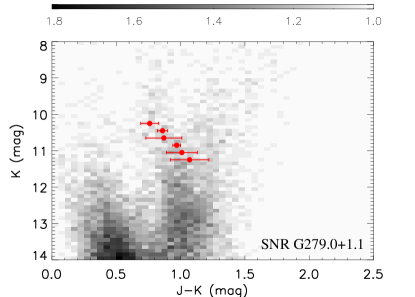
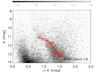
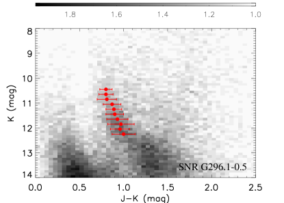
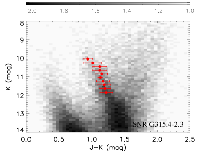
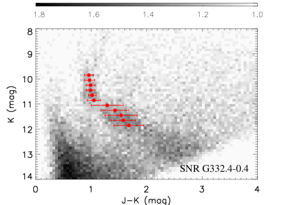
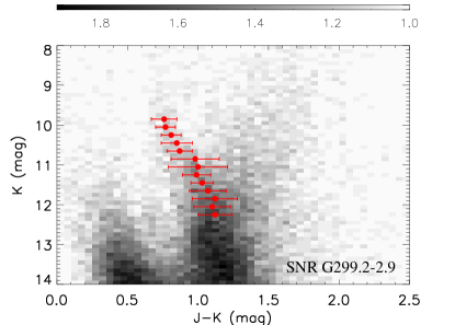
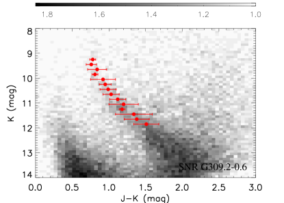
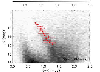
Figure 2: The CMDs within 0.5 deg² in the directions of 8 SNRs, the grey colours denote stellar densities in the logarithmic scale. The red dots and lines show the fitted location of the RC peak density and its extent with $1\sigma$.

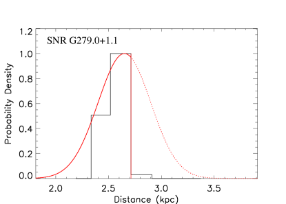
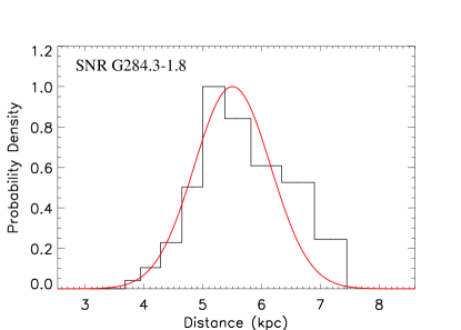
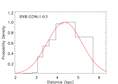
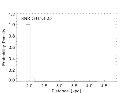
Figure 3: Left: The $\rm A_{V}$-D relation traced by RC stars along the direction of each SNR. The dashed line is $\rm A_{V}$ value of each SNR. The dotted lines are the uncertainties of $\rm A_{V}$. Right: Probability distribution over distance to the SNRs and the best-fit Gaussian model with the cutoffs. The red line in the right panel for G315.4-2.3 is the upper distance limit.

Fig. 3 continued

G279.0+1.1

The distance of G279.0+1.1 is estimated at 3 kpc by blast wave method and $\Sigma$-D relation (McKee & Cowie 1975; Stupar & Parker 2009). However, Stupar & Parker (2009) warned that this distance should be treated with caution since McKee & Cowie (1975)’s estimate depends on the initial explosion energy of progenitor star and $\Sigma$-D relation might have an error up to 40%. Our RC method estimates its distance as 2.7$\pm 0.3$ kpc which coincides with the previous measurements.

G284.3-1.8

G284.3-1.8 was suggested to associate with the pulsar PSR J1016-5857 (3 kpc， (Kargaltsev et al. 2013)) or the $\gamma$-ray binary 1FGL J1018.6-5856 (5.6${}_{-2.1}^{+4.6}$ kpc (Napoli et al. 2011)). We estimate its distance at 5.5$\pm 0.7$ kpc. The new distance indicates that G284.3-1.8 is not likely to be associated with the PSR J1016-5857 at 3 kpc.

G296.1-0.5

G296.1-0.5 is a middle-aged SNR with complex structures. Longmore et al. (1977) estimated its distance between 3 and 5 kpc from two independent ways of reddening measurements and kinematic method. Distances calculated by the $\Sigma$-D relation are 7.7, 6.6, 4.9 kpc from Caswell & Barnes (1983), Case & Bhattacharya (1998), and Clark et al. (1973), respectively. We show its distance of 4.3$\pm 0.8$ kpc, which further supports the results of Longmore et al. (1977) and Clark et al. (1973).

G315.4-2.3 (RCW 86)

Rosado et al. (1996) fitted the radial velocity of H_α with respect to the local standard of rest and converted it to a kinematic distance as 2.8$\pm 0.4$ kpc for G315.4-2.3 based on Galactic rotation curve. Sollerman et al. (2003) followed this method with the data of high spectroscopic resolution and constrained the distance as 2.3$\pm 0.2$ kpc. These distances were supported by the combination of the proper motion and the post-shock temperature (Helder et al. 2013). A smaller distance of $\rm 1.2_{-0.2}^{+0.2}$ kpc was determined with Sedov estimates (Bocchino et al. 2000). There is a cutoff in the probability distribution of distance because only the upper limit of $\rm A_{V}$ of G315.4-2.3 is in the range of $\rm A_{V}$ traced by the RC stars. Therefore,the red line in the right panel for G315.4-2.3 is the upper distance limit, estimated to be 2.0 kpc by the RC method.

G332.4-0.4 (RCW 103)

The kinematic distance based on HI absorption spectrum is about 3.3 kpc for RCW 103 (Caswell et al. 1975; Reynoso et al. 2004). Ruiz (1983) estimated its distances around 6.5 kpc by extinction measurement. However, the extinction traced by the RC stars infers that this SNR locates at 3.0$\pm 0.3$ kpc, which is consistent with the kinematic distances.

G299.2-2.9

We derive an RC distance of G299.2-2.9 at 2.8$\pm 0.8$ kpc for the first time. A low interstellar column density in the line of sight hinted a very nearby distance ($\sim$0.5 kpc) based on the ROSAT Position Sensitive Proportional Counter observation (Slane et al. 1996). However, spatially resolved spectroscopy with the Chandra X-Ray Observatory shows a higher hydrogen column density ($\rm N_{H}\sim 3.5\times 10^{21}cm^{-2}$), which suggested a distance of 2-11 kpc (Park et al. 2007). The RC distance is the best so far.

G308.4-1.4

Prinz & Becker (2012) gave a detailed analysis of the distance to G308.4-1.4: (1) the distance indicated by extinction is 5.9$\pm 2.0$ kpc; (2) a kinematic distance is $2.0\pm 0.6$ kpc or 12.5$\pm$0.7 kpc; (3) the Sedov-analysis-based distance is 9.8${}^{+0.9}_{-0.7}$ kpc. The RC distance of this SNR is 3.1$\pm 0.3$ kpc, which is consistent with the low limits of extinction distance and kinematic distance.

G309.2-0.6

HI absorption against G309.2-0.6 yielded a kinematic distance from 5.4$\pm 1.6$ to 14.1$\pm 0.7$ kpc (Gaensler et al. 1998). Rakowski et al. (2001) estimated the distance of this SNR to be $4\pm 2$ kpc from the foreground hydrogen column density. The distance measured by the RC method is 2.8$\pm 0.8$ kpc, which is consistent with the low limits of the previous measurements.

G309.8-2.6

We estimate the distance of G309.8-2.6 at 2.3$\pm 0.2$ kpc for the first time. The RC distance further supports that G309.8-2.6 is associated with the very young pulsar PSR J1357-6429 located at 2.5 kpc (Camilo et al. 2004).

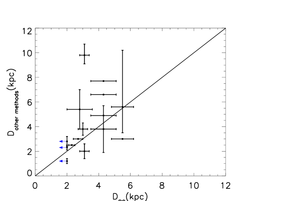
Figure 4: Comparison of the RC distances and the distances determined by other methods. The blue arrows represent the upper limit of distance for G315.4-2.3. The data is based on Table 1 and  2.

We compare the 9 RC distances of SNRs with the distances from other methods Fig. 4. Note that there might be several distance measurements for one SNR and a few of them without uncertainty estimates. The RC distances are generally consistent with the previous measurements within the error bars. The distance uncertainties from the RC method range from 10% to 30% and the accuracies of distances are significantly improved for 8 SNRs.