Statistical closure modeling for reduced-order models
of stationary systems by the ROMES method

Abstract

This work proposes a technique for constructing a statistical closure model for reduced-order models (ROMs) applied to stationary systems modeled as parameterized systems of algebraic equations. The proposed technique extends the reduced-order-model error surrogates (ROMES) method [13] to closure modeling. The original ROMES method applied Gaussian-process regression to construct a statistical model that maps cheaply computable error indicators (e.g., residual norm, dual-weighted residuals) to a random variable for either (1) the norm of the state error or (2) the error in a scalar-valued quantity of interest. Rather than target these two types of errors, this work proposes to construct a statistical model for the state error itself; it achieves this by constructing statistical models for the generalized coordinates characterizing both the in-plane error (i.e., the error in the trial subspace) and a low-dimensional approximation of the out-of-plane error. The former can be considered a statistical closure model, as it quantifies the error in the ROM generalized coordinates. Because any quantity of interest can be computed as a functional of the state, the proposed approach enables any quantity-of-interest error to be statistically quantified a posteriori, as the state-error model can be propagated through the associated quantity-of-interest functional. Numerical experiments performed on both linear and nonlinear stationary systems illustrate the ability of the technique (1) to improve (expected) ROM prediction accuracy by an order of magnitude, (2) to statistically quantify the error in arbitrary quantities of interest, and (3) to realize a more cost-effective methodology for reducing the error than a ROM-only approach in the case of nonlinear systems.

1 Introduction

Computational models of stationary systems modeled as parameterized systems of algebraic equations (e.g., those arising from the spatial discretization of a partial-differential-equations problem) are being increasingly used in complex decision-making scenarios. However, such scenarios are often many query or real time in nature. For example, uncertainty propagation often requires hundreds or thousands of solutions to the parameterized system in order to adequately characterize uncertainties; in-situ structural health monitoring requires such solutions to be computed in near real time. As a result, employing truly high-fidelity models characterized by large-scale systems of algebraic equations (e.g., arising from a fine spatial discretization) is often computationally intractable. To mitigate this computational burden, analysts often replace such computationally expensive high-fidelity ‘full-order models’ (FOMs) with computationally inexpensive surrogate models, which can be categorized as (i) data fits, which construct a regression model (e.g., via polynomial interpolation) that directly approximates the mapping from (parameter) inputs to (quantity-of-interest) outputs; (ii) lower-fidelity models, which introduce modeling simplifications (e.g., coarsened mesh, neglected physics); and (iii) reduced-order models (ROMs) constructed by performing a projection process on the equations governing the high-fidelity model to reduce the state-space dimensionality. Although typically more intrusive to implement, ROMs often yield more accurate approximations than data fits, and usually generate more significant computational gains than lower-fidelity models. For this reason, this work considers ROMs as the surrogate of interest. See, e.g., Refs. [5, 37, 19] for reviews on reduced-order-modeling techniques.

To rigorously apply ROMs within a decision-making scenario, their error with respect to the FOM must be quantified and properly accounted for in the ultimate prediction or assessment. In uncertainty quantification (UQ) applications, for example, the epistemic uncertainty introduced by the surrogate model should be statistically quantified [13, 29, 35]; on the other hand, risk-averse scenarios may demand a deterministic bound on a quantity of interest to ensure it does not exceed a specified threshold.

To this end, a variety of approaches have been proposed to quantify the error introduced by reduced-order models.

1. Error indicators. Error indicators are quantities that are informative of the error, yet are relatively inexpensive to compute. One example is the residual norm, i.e., the norm of the FOM residual evaluated at the ROM solution. This quantity can be used as an error indicator to guide greedy methods for parameter-space sampling [7, 6, 20, 1, 46, 48] and when employing ROMs within a trust-region setting [50, 49]. Alternatively, dual-weighted residuals employed in adjoint error estimation provide a first-order approximation of the error in a scalar-valued quantity of interest; they are often used for error estimation and adaptive mesh refinement, as well as in nonlinear model reduction [31, 8]. Unfortunately, error indicators alone are not easily amenable to UQ, as they generate a prediction of the error that is both deterministic and is often significantly biased.

2. A posteriori error bounds. These approaches derive deterministic bounds for the norm of either the state error or (quantity-of-interest) output error; they typically require evaluating the FOM residual at the ROM solution, as well as stability/continuity constant bounds, and dual quantities related to the quantity of interest. Such approaches aim to derive bounds that are rigorous, sharp, and inexpensive to compute [42]. However, these objectives are often competing, as improving bound sharpness can significantly increase the computational cost [23, 22]. Heuristic strategies to speed up error bound evaluation have been proposed [25, 28, 45], which yield error estimates rather than strict bounds. Alternatively, Ref. [18] proposes a hierarchical error estimator that can compute sharper estimates without requiring the computation of these constants, at the cost of solving a higher-dimensional ROM. Similarly to error indicators, deterministic error bounds are not directly useful for UQ applications, where a probability distribution for the ROM error is more amenable to quantifying the ROM-induced epistemic uncertainty.

3. Error models. These methods directly construct a regression model for the ROM error, i.e., they construct an approximation of the mapping from chosen regression-model inputs (or features) to a prediction of the ROM error. Nearly all approaches in this category employ the parameter inputs as the regression-model inputs [16, 33, 30, 14, 34]. These approaches are effective when the ROM error exhibits a low variability in the parameter space and the parameter space is low dimensional. However, the ROM error is often a highly oscillatory function of the inputs and the parameter space dimension is often high-dimensional in many practical settings, which can cause the approach to fail [33, 13]. The reduced-order-model error surrogates (ROMES) method [13] addresses this problem in the case of stationary systems. Rather than employing parameter inputs as regression-model inputs, the ROMES method instead employs the aforementioned error indicators and rigorous error bounds for this purpose. Because these quantities are cheaply computable, low-dimensional, and are often highly informative of the ROM error, the resulting error model is typically computationally inexpensive to evaluate, exhibits low variance, and can be sufficiently trained and validated using a relatively small amount of training data. Further, because the approach employs Gaussian-process regression, its prediction corresponds to a Gaussian random variable for the ROM error that can be readily integrated into UQ analyses; the variance of this random variable can be interpreted as the ROM-induced epistemic uncertainty. Ref. [41] extended this work to dynamical systems; rather than requiring the user to hand select a small number of error indicators, this approach employs high-dimensional regression models from machine learning (e.g., LASSO, random forests) to enable a large number of candidate error indicators to be used as inputs of the error model. Ref. [15] also extended the method in several ways: (1) it enabled the quantity-of-interest errors incurred by any approximate solution to be quantified, (2) it proposed a much wider range of inexpensive-to-compute residual-based features (e.g., gappy POD approximation of the residual), and (3) it applied a wide range of regression methods of varying capacity (e.g., support vector regression, artificial neural networks) within a model-selection framework.

Due to its ability to generate inexpensive-to-evaluate, low-variance, statistical error models that can be trained with relatively small amounts of training data, this work considers the ROMES method for constructing error models. We focus in particular on addressing one major shortcoming of the approach: it requires constructing of a separate error model for each quantity of interest. In many engineering applications, the analyst is often interested in field quantities (e.g., the solution field itself, the pressure field); constructing an error model for each element of the associated discrete error vector—whose dimension is the same as that of the full-order model—is computationally intractable. Alternatively, in exploratory contexts, the analyst may not have a priori knowledge of which quantities will be of interest; while ROMES models for each quantity of interest could in principle be constructed a posteriori in this case, this violates the natural offline–online decomposition leveraged by model reduction.

To address these shortcomings of the ROMES method, this work proposes to construct a statistical model for the state error itself. To avoid the need to construct a model for each element of the high-dimensional state error vector, the approach decomposes the state error into the in-plane error (i.e., the component belonging to the low-dimensional trial subspace) and the out-of-plane error (i.e., the component orthogonal to the trial subspace). Because the orthogonal complement of the trial subspace is high dimensional, the method employs a low-dimensional subspace—which is orthogonal to the trial subspace—to represent the out-of-plane error. Then, the method constructs a statistical error model for each generalized coordinate characterizing the low-dimensional representations of the in-plane and out-of-plane errors. The error model for the in-plane error can be considered a statistical closure model, as it aims to model the error in the preserved state variables (i.e., the generalized coordinates of the ROM solution) due to omitting the remaining variables from the formulation. The resulting error model can then be employed to statistically quantify the error in the entire state. Further, it can be used to generate an error model for any quantity of interest (including field quantities) a posteriori by propagating the state error through the associated quantity-of-interest functional. Numerical experiments demonstrate the ability of the method (1) to improve (expected) ROM prediction accuracy by an order of magnitude, (2) to statistically quantify the error in arbitrary quantities of interest a posteriori, and (3) to realize a more cost-effective methodology for reducing the error than a ROM-only approach in the case of nonlinear stationary systems.

We note that many existing works have proposed closure models for reduced-order models; see, e.g., Refs [43, 24, 39, 36, 47]. However, these methods are all applied to dynamical systems (typically in the context of fluid dynamics), and none of these techniques constructs a statistical model, which is essential for uncertainty quantification.

The paper is structured as follows. Section 2 formulates the problem by presenting the full-order model, the reduced-order model, and the state and quantity-of-interest errors associated with parameterized systems of algebraic equations. Section 3 describes the decomposition of the state error into in-plane and out-of-plane components, as well as computable dual-weighted-residuals that approximate the error in the associated generalized coordinates. Section 4 describes the proposed approach, i.e., the proposed statistical model (Section 4.1), the proposed error indicators (Section 4.2), a summary of Gaussian-process regression (Section 4.3), the application of the method to construct statistical error models for the state and quantities of interest (Section 4.5), and the offline–online decomposition of the approach (Section 4.6). Finally, Section 5 presents numerical experiments that assess the proposed method on both linear and nonlinear stationary systems, focusing particularly on model validation, the expected accuracy of the error models, and the computational efficiency of the proposed technique.

2 Problem formulation

This section presents the formulations of the FOM and ROM (with attendant state and quantity-of-interest errors) in the context of stationary systems.

2.1 Full-order model

In this work, the FOM corresponds to a stationary system modeled as a parameterized system of algebraic equations

(1) $$\mathbf{r}(\mathbf{x};\boldsymbol{\mu})=\mathbf{0},$$

where $\mathbf{r}:(\mathbf{w};\boldsymbol{\nu})\mapsto\mathbf{r}(\mathbf{w};\boldsymbol{\nu})$ with $\mathbf{r}:\mathbb{R}^{{N}}\times\mathcal{D}\rightarrow\mathbb{R}^{{N}}$ denotes the residual operator, $\boldsymbol{\mu}\in\mathcal{D}\subset\mathbb{R}^{{d}}$ denotes the system parameters, and $\mathbf{x}\equiv\mathbf{x}(\boldsymbol{\mu})\in\mathbb{R}^{{N}}$ denotes the state implicitly defined as the solution to (1) given parameters $\boldsymbol{\mu}$. If the residual operator $\mathbf{r}$ is linear in its first argument, then it takes the form

(2) $$\mathbf{r}:(\mathbf{w};\boldsymbol{\nu})\mapsto\mathbf{b}(\boldsymbol{\nu})-\mathbf{A}(\boldsymbol{\nu})\mathbf{w}$$

where $\mathbf{b}:\mathcal{D}\rightarrow\mathbb{R}^{{N}}$ and $\mathbf{A}:\mathcal{D}\rightarrow\mathbb{R}_{\star}^{{N}\times{N}}$ denote the (parameterized) right-hand-side vector and the system matrix, respectively, and $\mathbb{R}_{\star}^{m\times n}$ denotes the set of full-column rank $m\times n$ matrices (the non-compact Stiefel manifold). If instead the residual is nonlinear in its first argument, then Eq. (1) can be solved iteratively, e.g., via globalized Newton’s method by executing the following iterations: given initial guess $\mathbf{x}^{(0)}$, solve the linear system

$$\frac{\partial\mathbf{r}}{\partial\mathbf{w}}(\mathbf{x}^{(k-1)};\boldsymbol{\mu})\delta{\mathbf{x}}^{(k)}=-\mathbf{r}(\mathbf{x}^{(k-1)};\boldsymbol{\mu}),$$

and set

$$\mathbf{x}^{(k)}=\mathbf{x}^{(k-1)}+\alpha^{(k)}\delta{\mathbf{x}}^{(k)},$$

for $k=1,\ldots,K$, where $\alpha^{(k)}\in\mathbb{R}$ denotes a step length that can be computed to ensure global convergence (e.g., by satisfying the strong Wolfe conditions), and $K$ is determined by the satisfaction of a convergence criterion. Many practical scenarios in science and engineering are characterized by the following attributes:

1. The FOM is high-dimensional, i.e., ${N}$ is large. This arises when the FOM corresponds to the fine spatial discretization of a stationary partial-differential-equations problem, for example.

2. The primary goal of the analysis is compute quantities of interest that are functionals of the state, i.e., for a given parameter instance $\boldsymbol{\mu}$, the goal is to compute $\mathbf{q}(\boldsymbol{\mu})$ with $\mathbf{q}:\boldsymbol{\nu}\mapsto\mathbf{s}(\mathbf{x}(\boldsymbol{\nu});\boldsymbol{\nu})$ and $\mathbf{s}:\mathbb{R}^{{N}}\times\mathcal{D}\rightarrow\mathbb{R}^{s}$ denoting the quantity-of-interest functional.

3. The scenario is many-query in nature, i.e., it requires the computation of $\mathbf{q}(\boldsymbol{\mu})$ for $\boldsymbol{\mu}\in\mathcal{D}_{\mathrm{online}}\equiv\{\boldsymbol{\mu}^{\star}_{i}\}_{i=1}^{n_{\text{online}}}\subseteq\mathcal{D}$ with $n_{\text{online}}$ large. This arises in parameter studies, UQ applications, and design-optimization settings, for example.

In such cases, simply solving Eq. (1) for $\boldsymbol{\mu}\in\mathcal{D}_{\mathrm{online}}$ and subsequently computing the quantities of interest is usually computationally intractable, and a surrogate model is required to reduce the computational cost. As discussed in the introduction, this work focuses on applying reduced-order models for this purpose.

2.2 Reduced-order model

Reduced-order models reduce the dimensionality of the FOM governing equations (1) via projection. In particular, they seek approximate solutions $\mathbf{x}_{\text{ROM}}\approx\mathbf{x}$ in an $n$-dimensional affine trial subspace (with $n\ll{N}$), i.e.,

(3) $$\mathbf{x}_{\text{ROM}}(\boldsymbol{\mu})=\mathbf{x}_{\text{ref}}(\boldsymbol{\mu})+\mathbf{\Phi}\hat{\mathbf{x}}(\boldsymbol{\mu})\in\mathbf{x}_{\text{ref}}(\boldsymbol{\mu})+\mathcal{V},$$

with $\mathbf{x}_{\text{ROM}}:\mathcal{D}\rightarrow\mathbb{R}^{{N}}$. Here, $\mathbf{x}_{\text{ref}}:\mathcal{D}\rightarrow\mathbb{R}^{{N}}$ denotes a reference state (e.g., the mean of the snapshots in the case of proper orthogonal decomposition); the trial-basis matrix $\mathbf{\Phi}\equiv[\boldsymbol{\phi}_{1}\ \cdots\ \boldsymbol{\phi}_{n}]\in\mathbb{R}_{\star}^{{N}\times n}$ may be constructed by a variety of means (e.g., the reduced-basis method [40, 19, 37], proper orthogonal decomposition [21]); $\mathcal{V}\vcentcolon=\text{Ran}(\mathbf{\Phi})$ denotes the linear part of the affine trial subspace, where $\text{Ran}(\mathbf{A})$ denotes the range of matrix $\mathbf{A}$; and $\hat{\mathbf{x}}:\mathcal{D}\rightarrow\mathbb{R}^{n}$ denotes the generalized coordinates of the ROM solution.

Model-reduction approaches compute the approximate solution by substituting $\mathbf{x}\leftarrow\mathbf{x}_{\text{ROM}}$ in Eq. (1) and enforcing orthogonality of the residual to an $n$-dimensional linear test subspace, which yields the ROM governing equations

(4) $$\mathbf{\Psi}(\hat{\mathbf{x}};\boldsymbol{\mu})^{T}\mathbf{r}(\mathbf{x}_{\text{ref}}+\mathbf{\Phi}\hat{\mathbf{x}};\boldsymbol{\mu})=\mathbf{0},$$

where $\mathbf{\Psi}:\mathbb{R}^{n}\times\mathcal{D}\rightarrow\mathbb{R}_{\star}^{{N}\times n}$ denotes the test-basis matrix that generally may depend on the generalized coordinates and parameters. Common choices for the test basis include Galerkin projection, which employs $\mathbf{\Psi}=\mathbf{\Phi}$, and least-squares Petrov–Galerkin (LSPG) projection [6, 26, 10], which employs $\mathbf{\Psi}(\hat{\mathbf{x}};\boldsymbol{\mu})=\frac{\partial\mathbf{r}}{\partial\mathbf{w}}(\mathbf{x}_{\text{ref}}+\hat{\mathbf{x}};\boldsymbol{\mu})\mathbf{\Phi}$ and thus associates Eq. (4) with the necessary optimality conditions for a minimum-residual problem; see Ref. [9] for a detailed comparison of the two approaches in the context of nonlinear dynamical systems. When the residual operator is nonlinear in its first argument or nonaffine in (functions of) its second argument, additional ‘hyper-reduction’ techniques must be employed in order to ensure that the ROM equations (4) can be solved with a computational cost that is independent of the FOM dimension ${N}$. Such techniques include the empirical interpolation method (EIM) [4, 27, 17], its discrete variant DEIM [12, 2], gappy POD [44, 11], and missing point estimation [3].

Finally, we denote the ROM-predicted output as $\mathbf{q}_{\mathrm{ROM}}:\boldsymbol{\nu}\mapsto\mathbf{s}(\mathbf{x}_{\text{ROM}}(\boldsymbol{\nu});\boldsymbol{\nu})$. Critically, because the ROM solution approximates the FOM solution, the ROM will generally introduce both a state error and a quantity-of-interest error

(5) $${\boldsymbol{\delta}}_{\mathbf{x}} :\boldsymbol{\nu}\mapsto\mathbf{x}(\boldsymbol{\nu})-\mathbf{x}_{\text{ROM}}(\boldsymbol{\nu})\quad\text{and}\quad\boldsymbol{\delta}_{\mathbf{q}}:\boldsymbol{\nu}\mapsto\mathbf{q}(\boldsymbol{\nu})-\mathbf{q}_{\mathrm{ROM}}(\boldsymbol{\nu}),$$

respectively, with ${\boldsymbol{\delta}}_{\mathbf{x}}:\mathcal{D}\rightarrow\mathbb{R}^{{N}}$ and $\boldsymbol{\delta}_{\mathbf{q}}:\mathcal{D}\rightarrow\mathbb{R}^{s}.$

3 State error decomposition and approximation

The objective of this work is to compute statistical models of the state error ${\boldsymbol{\delta}}_{\mathbf{x}}$ and quantity-of-interest error $\boldsymbol{\delta}_{\mathbf{q}}$ in a manner that does not require identifying the quantities of interest a priori. We now present the mathematical framework that will be leveraged by the proposed method, which is presented in Section 4. In particular, this section (1) decomposes the state error ${\boldsymbol{\delta}}_{\mathbf{x}}$ into in-plane and out-of-plane errors (Section 3.1), (2) identifies low-dimensional subspaces for each of these error components (Section 3.2), (3) derives first-order estimates of the generalized coordinates characterizing these error components (Section 3.3), and (4) applies model reduction to inexpensively approximate these estimates (Section 3.4).

3.1 State error decomposition

We begin by defining the in-plane projector, which is the linear operator that computes the orthogonal projection onto the linear part $\mathcal{V}$ of the affine trial subspace, as

(6) $$\mathbf{P}^{\mathbin{\|}}\vcentcolon=\mathbf{\Phi}(\mathbf{\Phi}^{T}\mathbf{\Theta}\mathbf{\Phi})^{-1}\mathbf{\Phi}^{T}\mathbf{\Theta}.$$

Here, $\mathbf{\Theta}\in\mathrm{SPD}({N})$ is a matrix defining an inner product (e.g., the discrete counterpart to the inner product characterizing a Sobolev space) with $(\mathbf{w},\mathbf{y})_{\mathbf{\Theta}}\vcentcolon=\mathbf{w}^{T}\mathbf{\Theta}\mathbf{y}$ and $\|\mathbf{w}\|_{\mathbf{\Theta}}\vcentcolon=\sqrt{(\mathbf{w},\mathbf{w})_{\mathbf{\Theta}}}$, and $\mathrm{SPD}(N)$ denotes the set of $N\times N$ symmetric-positive-definite matrices. The in-plane projector $\mathbf{P}^{\mathbin{\|}}$ inherits standard properties of orthogonal projectors, i.e., optimality

(7) $$\mathbf{P}^{\mathbin{\|}}\mathbf{w}=\underset{\mathbf{y}\in\mathcal{V}}{\operatorname*{\arg\min}}\|\mathbf{w}-\mathbf{y}\|_{\mathbf{\Theta}};$$

orthogonality $(\mathbf{w}-\mathbf{P}^{\mathbin{\|}}\mathbf{w},\mathbf{y})_{\mathbf{\Theta}}=0$, $\forall\mathbf{w}\in\mathbb{R}^{{N}}$, $\forall\mathbf{y}\in\mathcal{V}$; and idempotency, $(\mathbf{P}^{\mathbin{\|}})^{2}=\mathbf{P}^{\mathbin{\|}}$.

The projector enables the state error to be decomposed as

(8) $${\boldsymbol{\delta}}_{\mathbf{x}}=\boldsymbol{\delta}^{\mathbin{\|}}+\boldsymbol{\delta}^{\perp},$$

where the in-plane error lies within the linear part $\mathcal{V}$ of the affine trial subspace and is defined as

(9) $$\begin{split}\boldsymbol{\delta}^{\mathbin{\|}}&:\boldsymbol{\nu}\mapsto\mathbf{P}^{\mathbin{\|}}{\boldsymbol{\delta}}_{\mathbf{x}}(\boldsymbol{\nu})\\ &:\mathcal{D}\rightarrow\mathcal{V},\end{split}$$

and the out-of-plane error is orthogonal to the linear subspace $\mathcal{V}$ and is defined as

(10) $$\begin{split}\boldsymbol{\delta}^{\perp}&:\boldsymbol{\nu}\mapsto{\boldsymbol{\delta}}_{\mathbf{x}}(\boldsymbol{\nu})-\mathbf{P}^{\mathbin{\|}}{\boldsymbol{\delta}}_{\mathbf{x}}(\boldsymbol{\nu})\\ &:\mathcal{D}\rightarrow\mathcal{V}^{\perp}.\end{split}$$

We note that $(\boldsymbol{\delta}^{\perp}(\boldsymbol{\mu}),\mathbf{y})_{\mathbf{\Theta}}=0$, $\forall\mathbf{y}\in\mathcal{V}$, $\forall\boldsymbol{\mu}\in\mathcal{D}$, and $(\boldsymbol{\delta}^{\perp}(\boldsymbol{\mu}),\boldsymbol{\delta}^{\mathbin{\|}}(\boldsymbol{\mu}))_{\mathbf{\Theta}}=0$, $\forall\boldsymbol{\mu}\in\mathcal{D}$. Figure 1 depicts this error decomposition graphically.

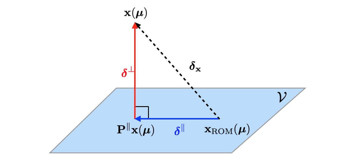
Figure 1: Graphical depiction of the decomposition of the state error ${\boldsymbol{\delta}}_{\mathbf{x}}\in\mathbb{R}^{{N}}$ into the in-plane error $\boldsymbol{\delta}^{\mathbin{\|}}\in\mathcal{V}$ and the out-of-plane error $\boldsymbol{\delta}^{\perp}\in\mathcal{V}^{\perp}$.

We note that the in-plane error $\boldsymbol{\delta}^{\mathbin{\|}}(\boldsymbol{\mu})$ can be interpreted as the closure error, as the in-plane error expresses the error in the ‘preserved variables’ (i.e., the solution component in the affine trial subspace $\mathbf{x}_{\text{ref}}+\mathcal{V}$) incurred by solving equations that omit the ‘neglected variables’ (i.e., the solution component in $\mathcal{V}^{\perp}$).

Remark 3.1 (Necessary conditions for zero in-plane error).

The in-plane (i.e., closure) error $\boldsymbol{\delta}^{\mathbin{\|}}(\boldsymbol{\mu})$ is zero if the residual $\mathbf{r}$ is linear in its first argument such that (2) holds and either: (1) Galerkin projection is employed (i.e., $\mathbf{\Psi}=\mathbf{\Phi}$), the system matrix is symmetric and positive definite (i.e., $\mathbf{A}(\boldsymbol{\mu})\in\mathrm{SPD}({N})$), and the chosen metric is equal to the system matrix (i.e., $\mathbf{\Theta}=\mathbf{A}(\boldsymbol{\mu})$, or (2) least-squares Petrov–Galerkin (LSPG) projection is employed (i.e., $\mathbf{\Psi}(\hat{\mathbf{x}};\boldsymbol{\mu})=\mathbf{A}(\boldsymbol{\mu})\mathbf{\Phi}$) and the chosen metric is equal to the associated normal-equations matrix (i.e., $\mathbf{\Theta}=\mathbf{A}(\boldsymbol{\mu})^{T}\mathbf{A}(\boldsymbol{\mu})$).

3.2 Low-dimensional representations of the state-error components

We aim to construct statistical models for both the in-plane error $\boldsymbol{\delta}^{\mathbin{\|}}$ and out-of-plane error $\boldsymbol{\delta}^{\perp}$; the former can be considered a statistical closure model. However, the offline cost of constructing a model for each of the ${N}$ elements of these error vectors is computationally costly, and the online complexity of evaluating these models is ${N}$-dependent. To mitigate this cost, we instead aim to construct a statistical model for generalized coordinates representing these errors in low-dimensional subspaces.

This is a straightforward task for the in-plane error, as $\boldsymbol{\delta}^{\mathbin{\|}}(\boldsymbol{\mu})\in\mathcal{V}$ with $\dim(\mathcal{V})=n\ll{N}$ by construction, and thus

(11) $$\boldsymbol{\delta}^{\mathbin{\|}}(\boldsymbol{\mu})=\mathbf{\Phi}\hat{\boldsymbol{\delta}}^{\mathbin{\|}}(\boldsymbol{\mu}),$$

where $\hat{\boldsymbol{\delta}}^{\mathbin{\|}}:\mathcal{D}\rightarrow\mathbb{R}^{n}$ denote the generalized coordinates of the in-plane error that—from the definition of the in-plane projector (6), in-plane error (9), and associated decomposition (11)—satisfies

(12) $$\hat{\boldsymbol{\delta}}^{\mathbin{\|}}:\boldsymbol{\nu}\mapsto(\mathbf{\Phi}^{T}\mathbf{\Theta}\mathbf{\Phi})^{-1}\mathbf{\Phi}^{T}\mathbf{\Theta}{\boldsymbol{\delta}}_{\mathbf{x}}(\boldsymbol{\nu}).$$

In contrast, the out-of-plane error satisfies $\boldsymbol{\delta}^{\perp}(\boldsymbol{\mu})\in\mathcal{V}^{\perp}$ with $\dim(\mathcal{V}^{\perp})={N}-n$. Because $n\ll{N}$, the subspace $\mathcal{V}^{\perp}$ is high-dimensional. To address this, we approximate the out-of-plane error in an $n^{\perp}$-dimensional (with $n^{\perp}\ll{N}$) linear subspace as

(13) $$\boldsymbol{\delta}^{\perp}(\boldsymbol{\mu})\approx\mathbf{\Phi}^{\perp}\hat{\boldsymbol{\delta}}^{\perp}(\boldsymbol{\mu})\in\hat{\mathcal{V}}^{\perp}\subset\mathcal{V}^{\perp}$$

with

(14) $$\hat{\boldsymbol{\delta}}^{\perp}:\boldsymbol{\nu}\mapsto\mathbf{P}^{\perp}\boldsymbol{\delta}^{\perp}(\boldsymbol{\nu}),$$

where

(15) $$\mathbf{P}^{\perp}\vcentcolon=\mathbf{\Phi}^{\perp}([\mathbf{\Phi}^{\perp}]^{T}\mathbf{\Theta}\mathbf{\Phi}^{\perp})^{-1}[\mathbf{\Phi}^{\perp}]^{T}\mathbf{\Theta}$$

is the orthogonal projection onto the linear subspace $\hat{\mathcal{V}}^{\perp}$; $\mathbf{\Phi}^{\perp}\in\mathbb{R}_{\star}^{{N}\times n^{\perp}}$ denotes the out-of-plane error basis matrix such that $\hat{\mathcal{V}}^{\perp}\vcentcolon=\text{Ran}(\mathbf{\Phi}^{\perp})$; and $\hat{\boldsymbol{\delta}}^{\perp}:\mathcal{D}\rightarrow\mathbb{R}^{n^{\perp}}$ denotes the generalized coordinates of the out-of-plane error that—from the definition of the out-of-plane error (10), the associated approximation (13), generalized-coordinate definition (14), and out-of-plane projector (15)—satisfies

(16) $$\hat{\boldsymbol{\delta}}^{\perp}(\boldsymbol{\mu})=([\mathbf{\Phi}^{\perp}]^{T}\mathbf{\Theta}\mathbf{\Phi}^{\perp})^{-1}[\mathbf{\Phi}^{\perp}]^{T}\mathbf{\Theta}{\boldsymbol{\delta}}_{\mathbf{x}}(\boldsymbol{\mu}),$$

where we have used $\mathbf{\Phi}^{T}\mathbf{\Theta}\mathbf{\Phi}^{\perp}=\mathbf{0}$.

Comparing Eqs. (12) and (16) and using $\mathbf{\Phi}^{T}\mathbf{\Theta}\mathbf{\Phi}^{\perp}=\mathbf{0}$ allows the definition of the (in-plane and out-of-plane) error generalized coordinates

(17) $$\hat{\boldsymbol{\delta}}:\boldsymbol{\nu}\mapsto\begin{bmatrix}\hat{\boldsymbol{\delta}}^{\mathbin{\|}}(\boldsymbol{\nu})\\ \hat{\boldsymbol{\delta}}^{\perp}(\boldsymbol{\nu})\end{bmatrix}=\mathbf{P}{\boldsymbol{\delta}}_{\mathbf{x}}(\boldsymbol{\mu})$$

where

(18) $$\mathbf{P}\vcentcolon=(\bar{\mathbf{\Phi}}^{T}\mathbf{\Theta}\bar{\mathbf{\Phi}})^{-1}\bar{\mathbf{\Phi}}^{T}\mathbf{\Theta}\in\mathbb{R}^{{\bar{n}}\times{N}},\quad\bar{\mathbf{\Phi}}\vcentcolon=\begin{bmatrix}\mathbf{\Phi}&\mathbf{\Phi}^{\perp}\end{bmatrix}\in\mathbb{R}_{\star}^{{N}\times{\bar{n}}}$$

and ${\bar{n}}\vcentcolon=n+n^{\perp}$.

Remark 3.2 (Out-of-plane basis matrix construction).

The out-of-plane basis matrix $\mathbf{\Phi}^{\perp}$ can be constructed by a variety of means. For example, if $\mathbf{\Phi}$ corresponds to a truncated proper orthogonal decomposition (POD) basis, then $\mathbf{\Phi}^{\perp}$ can be set to the (discarded) $n+1$ to ${\bar{n}}$ POD modes; this idea has also been employed in the context of ROM error estimation [45]. Alternatively, the basis can be constructed by computing the projection error of FOM solutions over a parameter set $\boldsymbol{\mu}\in\mathcal{D}_{\textrm{out-of-plane}}\subset\mathcal{D}$ such that $\hat{\mathcal{V}}^{\perp}\subseteq\mathrm{span}\{\mathbf{x}(\boldsymbol{\mu})-\mathbf{x}_{\text{ref}}-\mathbf{P}^{\mathbin{\|}}\mathbf{x}(\boldsymbol{\mu})\}_{\boldsymbol{\mu}\in\mathcal{D}_{\textrm{out-of-plane}}}$.

3.3 Dual-weighted-residual error estimation

We now derive first-order approximations for the in-plane-error generalized coordinates $\hat{\boldsymbol{\delta}}^{\mathbin{\|}}$ and out-of-plane-error general coordinates $\hat{\boldsymbol{\delta}}^{\perp}$. Assuming the residual is twice continuously differentiable, we can approximate the residual of the FOM solution to first order about the residual of the ROM solution as

(19) $$\mathbf{0}=\mathbf{r}(\mathbf{x}(\boldsymbol{\mu});\boldsymbol{\mu})=\mathbf{r}(\mathbf{x}_{\text{ROM}}(\boldsymbol{\mu});\boldsymbol{\mu})+\frac{\partial\mathbf{r}}{\partial\mathbf{w}}(\mathbf{x}_{\text{ROM}}(\boldsymbol{\mu});\boldsymbol{\mu}){\boldsymbol{\delta}}_{\mathbf{x}}(\boldsymbol{\mu})+O(\|{\boldsymbol{\delta}}_{\mathbf{x}}(\boldsymbol{\mu})\|^{2}),\quad\text{as}\ \|{\boldsymbol{\delta}}_{\mathbf{x}}(\boldsymbol{\mu})\|\rightarrow 0.$$

Note that the high-order term is zero if the residual is linear in its first argument, i.e., if (2) holds. Solving for the state error yields

(20) $${\boldsymbol{\delta}}_{\mathbf{x}}(\boldsymbol{\mu})=-\left[\frac{\partial\mathbf{r}}{\partial\mathbf{w}}(\mathbf{x}_{\text{ROM}}(\boldsymbol{\mu});\boldsymbol{\mu})\right]^{-1}\mathbf{r}(\mathbf{x}_{\text{ROM}}(\boldsymbol{\mu});\boldsymbol{\mu})+O(\|{\boldsymbol{\delta}}_{\mathbf{x}}(\boldsymbol{\mu})\|^{2}),\quad\text{as}\ \|{\boldsymbol{\delta}}_{\mathbf{x}}(\boldsymbol{\mu})\|\rightarrow 0.$$

Substituting Eq. (20) in Eq. (17) yields

(21) $$\hat{\boldsymbol{\delta}}(\boldsymbol{\mu})=-\mathbf{P}\left[\frac{\partial\mathbf{r}}{\partial\mathbf{w}}(\mathbf{x}_{\text{ROM}}(\boldsymbol{\mu});\boldsymbol{\mu})\right]^{-1}\mathbf{r}(\mathbf{x}_{\text{ROM}}(\boldsymbol{\mu});\boldsymbol{\mu})+O(\|{\boldsymbol{\delta}}_{\mathbf{x}}(\boldsymbol{\mu})\|^{2}),\quad\text{as}\ \|{\boldsymbol{\delta}}_{\mathbf{x}}(\boldsymbol{\mu})\|\rightarrow 0.$$

Defining the $i$th dual $\mathbf{p}_{i}:\mathcal{D}\rightarrow\mathbb{R}^{{N}}$, $i=1,\ldots,{\bar{n}}$ as the solution to the ${N}$-dimensional system of linear equations

(22) $$\left[\frac{\partial\mathbf{r}}{\partial\mathbf{w}}(\mathbf{x}_{\text{ROM}}(\boldsymbol{\mu});\boldsymbol{\mu})\right]^{T}\mathbf{p}_{i}(\boldsymbol{\mu})=-\mathbf{P}^{T}\mathbf{e}_{i},\quad i=1,\ldots,{\bar{n}},$$

where $\mathbf{e}_{i}\in\{0,1\}^{{N}}$ denotes the $i$th canonical unit vector, we can express the $i$th error generalized coordinate as

(23) $$\hat{\delta}_{i}(\boldsymbol{\mu})=\mathbf{p}_{i}(\boldsymbol{\mu})^{T}\mathbf{r}(\mathbf{x}_{\text{ROM}}(\boldsymbol{\mu});\boldsymbol{\mu})+O(\|{\boldsymbol{\delta}}_{\mathbf{x}}(\boldsymbol{\mu})\|^{2}),\quad\text{as}\ \|{\boldsymbol{\delta}}_{\mathbf{x}}(\boldsymbol{\mu})\|\rightarrow 0,\quad i=1,\ldots,{\bar{n}}.$$

3.4 Reduced-order model approximation to dual-weighted-residual error estimates

Dual problems (22) are linear, even if the original problem (1) is nonlinear; however, their dimension ${N}$ remains the same as that of the full-order model. Thus, employing the associated dual vectors for a posteriori error modeling as suggested by Eq. (23) is computationally expensive.

To mitigate this cost, we propose to approximate these duals via model reduction in analogue to the approach described in Section 2.2 for approximating the state. First, we approximate the duals as $\mathbf{p}_{i}\approx\tilde{\mathbf{p}}_{i}$, $i=1,\ldots,{\bar{n}}$, where

(24) $$\tilde{\mathbf{p}}_{i}(\boldsymbol{\mu})=\mathbf{\Phi}_{p,{i}}\hat{\mathbf{p}}_{i}(\boldsymbol{\mu}),\quad i=1,\ldots,{\bar{n}}$$

where $\mathbf{\Phi}_{p,{i}}\in\mathbb{R}_{\star}^{{N}\times n_{p,{i}}}$ denote the dual trial-basis matrices, $\hat{\mathbf{p}}_{i}:\mathcal{D}\rightarrow\mathbb{R}^{n_{p,{i}}}$, and $n_{p,{i}}\ll{N}$ for $i=1,\ldots,{\bar{n}}$. As in the case of the trial-basis matrix $\mathbf{\Phi}$, the trial-basis matrices $\mathbf{\Phi}_{p,{i}}$, $i=1,\ldots,{\bar{n}}$ can be constructed by a variety of means, e.g., the reduced-basis method, POD. We then substitute $\mathbf{p}_{i}\leftarrow\tilde{\mathbf{p}}_{i}$ in Eqs. (22) and enforce orthogonality of the residual to the range of associated test basis matrices $\mathbf{\Psi}_{p,{i}}(\boldsymbol{\mu})\in\mathbb{R}_{\star}^{{N}\times n_{p,{i}}}$, $i=1,\ldots,{\bar{n}}$ to obtain the ROM systems of equations

(25) $$[\mathbf{\Psi}_{p,{i}}(\boldsymbol{\mu})]^{T}\left[\frac{\partial\mathbf{r}}{\partial\mathbf{w}}(\mathbf{x}_{\text{ROM}}(\boldsymbol{\mu});\boldsymbol{\mu})\right]^{T}\mathbf{\Phi}_{p,{i}}\hat{\mathbf{p}}_{i}(\boldsymbol{\mu})=-[\mathbf{\Psi}_{p,{i}}(\boldsymbol{\mu})]^{T}\mathbf{\Theta}\mathbf{\Phi}(\mathbf{\Phi}^{T}\mathbf{\Theta}\mathbf{\Phi})^{-1}\mathbf{e}_{i},$$

for $i=1,\ldots,{\bar{n}}$, whose solutions define the generalized coordinates $\hat{\mathbf{p}}_{i}$, $i=1,\ldots,{\bar{n}}$.

As before, a Galerkin projection corresponds to $\mathbf{\Psi}_{p,{i}}=\mathbf{\Phi}_{p,{i}}$, $i=1,\ldots,{\bar{n}}$, while an LSPG projection corresponds to $\mathbf{\Psi}_{p,{i}}(\boldsymbol{\mu})=\left[\frac{\partial\mathbf{r}}{\partial\mathbf{w}}(\mathbf{x}_{\text{ROM}}(\boldsymbol{\mu});\boldsymbol{\mu})\right]^{T}\mathbf{\Phi}_{p,{i}}$ $i=1,\ldots,{\bar{n}}$. Again, if the residual operator is nonlinear in the state or nonaffine in functions of the parameter inputs, then hyper-reduction is required to ensure the cost of assembling the linear systems in Eqs. (25) does not scale with the dimension ${N}$.

Now, substituting $\mathbf{p}_{i}\leftarrow\tilde{\mathbf{p}}_{i}$ Eqs. (23) and ignoring high-order terms yields cheaply computable approximations to the in-plane and out-of-plane error generalized coordinates

(26) $$\hat{\delta}_{i}(\boldsymbol{\mu})\approx[\tilde{\mathbf{p}}_{i}(\boldsymbol{\mu})]^{T}\mathbf{r}(\mathbf{x}_{\text{ROM}}(\boldsymbol{\mu});\boldsymbol{\mu}),\quad i=1,\ldots,{\bar{n}}.$$

Note that the approximation is induced by the use of a model reduction to approximate the duals, as well as truncation error in the case of nonlinear FOM equations (1). The next section describes how this approximation to the error generalized coordinates can be used to construct a statistical model of the state error.

Remark 3.3 (Unique v. shared dual bases).

The strategy outlined above for applying model reduction to the dual problems requires the construction of ${\bar{n}}$ dual trial-basis matrices and dual test-basis matrices $\mathbf{\Phi}_{p,{i}}$ and $\mathbf{\Psi}_{p,{i}}$, $i=1,\ldots,{\bar{n}}$, respectively. If each of these basis matrices is unique, then the cost of solving Eqs. (25) is approximately $2/3\sum_{i=1}^{{\bar{n}}}n_{p,{i}}^{3}+2\sum_{i=1}^{{\bar{n}}}n_{p,{i}}^{2}$; this cost is small if each dual trial-basis matrix dimension $n_{p,{i}}$ is small. However, each of the basis matrices must be trained independently; in the event of limited training, these basis matrices individually may be too low-dimensional to generate accurate dual approximations $\tilde{\mathbf{p}}_{i}$, which can lead to large approximation errors.

Alternatively, one may employ a single ‘shared’ dual trial-basis matrix $\mathbf{\Phi}_{p}\in\mathbb{R}_{\star}^{{N}\times n_{p}}$ and test-basis matrix $\mathbf{\Psi}_{p}\in\mathbb{R}_{\star}^{{N}\times n_{p}}$ such that $\mathbf{\Phi}_{p,{i}}=\mathbf{\Phi}_{p}$ and $\mathbf{\Psi}_{p,{i}}=\mathbf{\Psi}_{p}$, $i=1,\ldots,{\bar{n}}$. In this case—because each of the linear systems (25) is characterized by the same system matrix—the cost of solving the resulting systems is approximately $2/3n_{p}^{3}+2{\bar{n}}n_{p}^{2}$. In many cases, this cost is significant, as the dimension $n_{p}$ is typically large, due to the fact that the basis is constructed from jointly training all duals; in the worst case, if $n_{p}=\sum_{i=1}^{\bar{n}}n_{p,{i}}$, then the cost is $2/3(\sum_{i=1}^{\bar{n}}n_{p,{i}})^{3}+2{\bar{n}}(\sum_{i=1}^{\bar{n}}n_{p,{i}})^{2}$. On the other hand, this approach often requires less training to compute a trial-basis matrix with good approximation properties, as information across all dual solutions informs the basis.

4 ROMES error models

We now leverage the framework presented in Section 3 to describe the application of the ROMES method [13] to construct statistical models of the in-plane and out-of-plane error generalized coordinates using indicators corresponding to the approximated dual-weighted residuals. Section 4.1 describes the formulation for the statistical model, Section 4.2 describes the error indicator (i.e., feature) we employ, Section 4.3 provides an overview of Gaussian-process regression, which is the technique we employ to construct the statistical model, Section 4.5 describes the application of ROMES error models to obtain statistical models for the state and quantities-of-interest errors, and Section 4.6 describes the offline/online computational strategy employed to realize the method in practice.

4.1 Statistical model

Our objective is to construct a low-dimensional, statistical model of the high-dimensional, deterministic, and generally unknown ROM error. The probability distribution of the random variable representing the ROM error reflects the epistemic uncertainty about its value. Define a probability space $(\Omega,\mathcal{F},P)$. We aim to approximate the high-dimensional deterministic mappings

(27) $$\begin{split}&m_{i}:\boldsymbol{\nu}\mapsto\hat{\delta}_{i}(\boldsymbol{\nu}),\quad i=1,\ldots,{\bar{n}}\end{split}$$

with $m_{i}:\mathcal{D}\rightarrow\mathbb{R}$ and ${d}$ possibly large, by univariate stochastic mappings

(28) $$\begin{split}&\tilde{m}_{i}:\rho_{i}(\boldsymbol{\nu})\mapsto\tilde{\delta}_{i}(\boldsymbol{\nu}),\quad i=1,\ldots,{\bar{n}}\end{split}$$

respectively, where $\rho_{i}:\mathcal{D}\rightarrow\mathbb{R}$, $i=1,\ldots,{\bar{n}}$ denote error indicators and $\tilde{\delta}_{i}(\boldsymbol{\nu}):\Omega\rightarrow\mathbb{R}$, $i=1,\ldots,{\bar{n}}$ denote random variables for the error generalized coordinates. The stochastic mapping should satisfy the following desiderata (see Refs. [13, 15]):

1. the error indicators are cheaply computable given any $\boldsymbol{\mu}\in\mathcal{D}$;

2. the stochastic mappings exhibit low variance, i.e., $\mathbb{E}[(\tilde{m}_{i}(\rho_{i}(\boldsymbol{\mu}))-\mathbb{E}[\tilde{m}_{i}(\rho_{i}(\boldsymbol{\mu}))])^{2}]$ is ‘small’ for all $\boldsymbol{\mu}\in\mathcal{D}$ (this ensures the ROM-induced epistemic uncertainty is small); and

3. the stochatic mappings are validated, i.e., the (empirical) distribution of test data is ‘close’ to the (reference) distribution prescribed by the stochastic mappings (using, e.g., prediction intervals, the Komolgorov–Smirnov test).

We now describe choices of error indicators and stochastic-mapping methods that lead to statistical models satisfying the above conditions.

4.2 Error indicators

The error indicator should be selected so that it is both cheaply computable (Condition 1 above) and can lead to a low-variance stochastic mapping (Condition 2 above); the latter condition implies that the error indicator should be informative of the error such that the mean of the stochastic mapping can explain most of the variance in the observed error.

Inspired by the analysis of Section 3, and Eq. (26) in particular, we propose employing the approximated dual-weighted residual as an error indicator, i.e.,

(29) $$\rho_{i}(\boldsymbol{\mu})=[\tilde{\mathbf{p}}_{i}(\boldsymbol{\mu})]^{T}\mathbf{r}(\mathbf{x}_{\text{ROM}}(\boldsymbol{\mu});\boldsymbol{\mu}),\quad i=1,\ldots,{\bar{n}}.$$

From Eq. (26), we can see that $\hat{\delta}_{i}(\boldsymbol{\mu})\approx\rho_{i}(\boldsymbol{\mu})$, where the approximation arises both to the use of model reduction to approximate the duals and truncation error when the residual is nonlinear in the state.

4.3 Gaussian-process regression

As in Ref. [13], we propose to construct the stochastic mappings $\tilde{m}_{i}$, $i=1,\ldots,{\bar{n}}$ using Gaussian process (GP) kernel regression [38], which is a supervised machine learning method. We first provide a brief review of this technique. A GP is a collection of random variables such that any finite number of them has a joint Gaussian distribution. GP kernel regression computes this GP by Bayesian inference using a kernel function and training data $\mathcal{T}=\{(\boldsymbol{x}_{i},y_{i})\}_{i=1}^{n_{\text{train}}}$, where $\boldsymbol{x}_{i}\in\mathbb{R}^{n_{\boldsymbol{x}}}$ and $y_{i}\in\mathbb{R}$ denote the $i$th instance of the features and response, respectively. We consider a single prediction point characterized by features $\boldsymbol{x}^{\star}\in\mathbb{R}^{n_{\boldsymbol{x}}}$, as we treat all predictions as arising from independent samples of the GP. First, the approach sets the prior distribution to

(30) $$\tilde{y}_{\text{prior}}(\underline{\mathbf{x}})\sim\mathcal{N}\left({\mathbf{H}\boldsymbol{\beta}},\mathbf{K}(\underline{\mathbf{x}},\underline{\mathbf{x}})+\sigma^{2}\mathbf{I}\right).$$

Here, $\underline{\mathbf{x}}\vcentcolon=[\underline{\boldsymbol{x}}_{1}\ \cdots\ \underline{\boldsymbol{x}}_{n_{\text{train}}+1}]^{T}\in\mathbb{R}^{(n_{\text{train}}+1)\times n_{\boldsymbol{x}}}$ with $\underline{\boldsymbol{x}}_{i}=\boldsymbol{x}_{i}$, $i=1,\ldots,n_{\text{train}}$ and $\underline{\boldsymbol{x}}_{n_{\text{train}}+1}=\boldsymbol{x}^{\star}$; element $(i,j)$ of the matrix $\mathbf{H}\in\mathbb{R}^{(n_{\text{train}}+1)\times n_{h}}$ is $[\mathbf{H}]_{ij}\vcentcolon=h_{j}(\underline{\boldsymbol{x}}_{i})$ with $h_{j}:\mathbb{R}^{n_{\boldsymbol{x}}}\rightarrow\mathbb{R}$, $j=1,\ldots,n_{h}$ denoting the considered basis functions (e.g., polynomials); $\boldsymbol{\beta}\in\mathbb{R}^{n_{h}}$ denotes the basis-expansion coefficients; and $\sigma^{2}$ denotes the additive noise arising from the non-uniqueness of the mapping from the features to the response. Element $(i,j)$ of the kernel matrix $\mathbf{K}(\mathbf{w},\mathbf{z})$ with $\mathbf{w}\vcentcolon=[\boldsymbol{w}_{1}\ \cdots\ \boldsymbol{w}_{n_{w}}]$ and $\mathbf{z}\vcentcolon=[\boldsymbol{z}_{1}\ \cdots\ \boldsymbol{z}_{n_{z}}]$ is

(31) $$[\mathbf{K}(\mathbf{w},\mathbf{z})]_{ij}\vcentcolon=\kappa(\boldsymbol{w}_{i},\boldsymbol{z}_{j}),\quad i=1,\ldots,n_{w},\ j=1,\ldots,n_{z}$$

and many choices of the kernel function $\kappa$ exist. The kernel function is typically characterized by its own hyperparameters $\boldsymbol{\theta}_{\kappa}$, e.g., the length scale in the case of the squared exponential kernel. Given the training data $\mathcal{T}$ and fixed values of the coefficients $\boldsymbol{\beta}$, noise variance $\sigma^{2}$, and kernel hyperparameters $\boldsymbol{\theta}_{\kappa}$, the prediction corresponds to a random variable with posterior distribution

(32) $$\tilde{y}(\boldsymbol{x}^{\star};\boldsymbol{\theta})\sim\mathcal{N}\left(\nu(\boldsymbol{x}^{\star}),\bar{\sigma}^{2}(\boldsymbol{x}^{\star})\right)$$

with

(33) $$\nu(\boldsymbol{x}^{\star})\vcentcolon=\mathbf{K}(\boldsymbol{x}^{\star},\mathbf{x})(\mathbf{K}(\mathbf{x},\mathbf{x})+\sigma^{2}\mathbf{I})^{-1}\mathbf{y}+{[h_{1}(\boldsymbol{x}^{\star})\ \cdots\ h_{n_{h}}(\boldsymbol{x}^{\star})]\boldsymbol{\beta}}$$

(34) $$\bar{\sigma}^{2}(\boldsymbol{x}^{\star})\vcentcolon=\mathbf{K}(\boldsymbol{x}^{\star},\boldsymbol{x}^{\star})-\mathbf{K}(\boldsymbol{x}^{\star},\mathbf{x})(\mathbf{K}(\mathbf{x},\mathbf{x})+\sigma^{2}\mathbf{I})^{-1}\mathbf{K}(\mathbf{x},\boldsymbol{x}^{\star})+\sigma^{2},$$

where $\mathbf{y}\vcentcolon=\left[y_{1}\ \cdots\ y_{n_{\text{train}}}\right]^{T}$ and $\mathbf{x}\vcentcolon=[\boldsymbol{x}_{1}\ \cdots\ \boldsymbol{x}_{n_{\text{train}}}]$. Indeed, computing the posterior using the training data is a simple operation derived from conditioning a joint Gaussian distribution. The parameters $\boldsymbol{\beta}$, $\sigma^{2}$, and hyperparameters characterizing the kernel $\boldsymbol{\theta}_{\kappa}$ can be set in a variety of ways, e.g., via maximum likelihood estimation (as in Ref. [13]), cross-validation.

4.4 Gaussian-process ingredients and cross-validation for ROMES

In this work, we specify the GP ingredients as follows. Following the ROMES method [13] and the presentation of Section 4.1, we propose to apply GP regression to (independently) construct each of the mappings $\tilde{m}_{i}$, $i=1,\ldots,{\bar{n}}$, wherein the feature corresponds to the prescribed error indicator (i.e., $\boldsymbol{x}=\rho_{i}$ with $n_{\boldsymbol{x}}=1$), and the response corresponds to the error generalized coordinate (i.e., $y=\hat{\delta}_{i}$). Eqs. (26) and (29) illustrate that the relationship between the features and the response is approximately linear in this case; it is exactly linear if the approximated dual is exact (i.e., $\mathbf{p}_{i}=\tilde{\mathbf{p}}_{i}$) and the when the residual operator $\mathbf{r}$ is linear in its first argument (i.e., Eq. (2) holds). Thus, we select the basis functions in the mean of the prior distribution (30) to enable linear responses, i.e., $h_{1}:\rho_{i}\mapsto 1$, $h_{2}:\rho_{i}\mapsto\rho_{i}$ with $n_{h}=2$.

For training the ROMES models, we employ training data comprising indicator–error pairs computed at ROMES-training parameter instances $\mathcal{D}_{\mathrm{ROMES}}\subset\mathcal{D}$ with $|\mathcal{D}_{\mathrm{ROMES}}|=n_{\text{train}}$, i.e., the training data for model $\tilde{m}_{i}$ corresponds to

(35) $$\mathcal{T}_{i}\vcentcolon=\{(\rho_{i}(\boldsymbol{\mu}),\hat{\delta}_{i}(\boldsymbol{\mu}))\}_{\boldsymbol{\mu}\in\mathcal{D}_{\mathrm{ROMES}}},\quad i=1,\ldots,{\bar{n}}.$$

Recall that the error generalized coordinates $\hat{\boldsymbol{\delta}}(\boldsymbol{\mu})$ can be computed from Eq. (17); this expression requires computing the state error ${\boldsymbol{\delta}}_{\mathbf{x}}(\boldsymbol{\mu})$, which in turn requires computing both the FOM state $\mathbf{x}(\boldsymbol{\mu})$ and ROM state $\mathbf{x}_{\text{ROM}}(\boldsymbol{\mu})$.

Given training data $\mathcal{T}_{i}$, we train model $\tilde{m}_{i}$ as follows: we determine the hyperparmeters $\boldsymbol{\theta}_{i}\equiv(\sigma_{i}^{2},\boldsymbol{\theta}_{\kappa,i})$ using $K$-fold cross validation with specialized loss functions that target different interpretations of statistical validation (condition 3 in Section 4.1), and we determine the coefficients $\boldsymbol{\beta}_{i}$ using maximum likelihood estimation. In particular, we first separate the ROMES training data $\mathcal{T}_{i}$ into $K$ non-overlapping subsets $\mathcal{T}_{i,j}$, $j=1,\ldots,K$ such that $\mathcal{T}_{i}=\cup_{j=1}^{K}\mathcal{T}_{i,j}$ and $\mathcal{T}_{i,j}\cap\mathcal{T}_{i,k}=\emptyset$, $j\neq k$. We then define a set of candidate hyperparameter values $\boldsymbol{\Theta}$. For each candidate value of the hyperparameters $\boldsymbol{\theta}\equiv(\sigma^{2},\boldsymbol{\theta}_{\kappa})\in\boldsymbol{\Theta}$, we compute the values of basis-expansion coefficients using maximum likelihood estimation as

(36) $$\boldsymbol{\beta}_{i,j}(\boldsymbol{\theta})=\left([\mathbf{1}\ \boldsymbol{\rho}_{i,j}]^{T}(\mathbf{K}(\boldsymbol{\rho}_{i,j},\boldsymbol{\rho}_{i,j})+\sigma^{2}\mathbf{I})^{-1}[\mathbf{1}\ \boldsymbol{\rho}_{i,j}]\right)^{-1}[\mathbf{1}\ \boldsymbol{\rho}_{i,j}]^{T}(\mathbf{K}(\boldsymbol{\rho}_{i,j},\boldsymbol{\rho}_{i,j})+\sigma^{2}\mathbf{I})^{-1}\hat{\boldsymbol{\delta}}_{i,j},$$

where $\boldsymbol{\rho}_{i,j}\in\mathbb{R}^{|\mathcal{T}_{i}\setminus\mathcal{T}_{i,j}|}$ and $\hat{\boldsymbol{\delta}}_{i,j}\in\mathbb{R}^{|\mathcal{T}_{i}\setminus\mathcal{T}_{i,j}|}$ denote the vectorized features and responses associated with training set $\mathcal{T}_{i}\setminus\mathcal{T}_{i,j}$, and $\mathbf{1}$ denotes a vector of ones. Note that we have suppressed the dependence of the kernel matrix $\mathbf{K}$ on the hyperparameters $\boldsymbol{\theta}_{\kappa}$ for notational simplicity. The values $\boldsymbol{\theta}$ and $\boldsymbol{\beta}_{i,j}(\boldsymbol{\theta})$ define a candidate ROMES model $\tilde{m}_{i,j}$ characterized by

(37) $$\tilde{m}_{i,j}(\rho_{i}(\boldsymbol{\mu});\boldsymbol{\theta})=\tilde{\delta}_{i,j}(\boldsymbol{\mu};\boldsymbol{\theta})\sim\mathcal{N}\left(\nu_{i,j}(\rho_{i}(\boldsymbol{\mu});\boldsymbol{\theta}),\bar{\sigma}_{i,j}^{2}(\rho_{i}(\boldsymbol{\mu});\boldsymbol{\theta})\right),\quad i=1,\ldots,{\bar{n}}$$

with

(38) $$\nu_{i,j}(\rho;\boldsymbol{\theta})\vcentcolon=\mathbf{K}(\rho,\boldsymbol{\rho}_{i,j})(\mathbf{K}(\boldsymbol{\rho}_{i,j},\boldsymbol{\rho}_{i,j})+\sigma^{2}\mathbf{I})^{-1}\hat{\boldsymbol{\delta}}_{i,j}+[1\ \rho]\boldsymbol{\beta}_{i,j}(\boldsymbol{\theta})$$

(39) $$\bar{\sigma}_{i,j}^{2}(\rho;\boldsymbol{\theta})\vcentcolon=\mathbf{K}(\rho,\rho)-\mathbf{K}(\rho,\boldsymbol{\rho}_{i,j})(\mathbf{K}(\boldsymbol{\rho}_{i,j},\boldsymbol{\rho}_{i,j})+\sigma^{2}\mathbf{I})^{-1}\mathbf{K}(\boldsymbol{\rho}_{i,j},\rho)+\sigma^{2}.$$

Subsequently, each candidate value of the hyperparameters $\boldsymbol{\theta}\in\boldsymbol{\Theta}$ is assigned a loss $L_{i}(\boldsymbol{\theta})$ with

(40) $$L_{i}(\boldsymbol{\theta})\equiv\frac{1}{K}\sum_{j=1}^{K}L_{i,j}(\boldsymbol{\theta}),$$

where $L_{i,j}(\boldsymbol{\theta})$ denotes the loss for the $i$th ROMES model on the $j$th validation set corresponding to hyperparameters $\boldsymbol{\theta}$. We then set the hyperparameters for the $i$th ROMES model to be the minimizer of the associated loss over the validation set, i.e.,

(41) $$\boldsymbol{\theta}_{i}=\underset{\boldsymbol{\theta}\in\boldsymbol{\Theta}}{\arg\min}L_{i}(\boldsymbol{\theta}).$$

One benefit of this cross-validation approach is that it admits flexibility in selecting the loss function $L_{i,j}(\boldsymbol{\theta})$, which determines hyperparameter selection. Because one of our objectives is to achieve statistical validation (condition 3 in Section 4.1), we can define this loss function to align with different notions of statistical validation; this is particularly important when the errors do not exhibit a Gaussian distribution, as this case precludes the ability to achieve statistical validation in every possible metric. We thus propose the following loss functions:

1. the negative log-likelihood

   (42) $$L_{\text{likelihood},i,j}(\boldsymbol{\theta})\vcentcolon=\frac{|\mathcal{T}_{i,j}|}{2}\ln(2\pi)+\frac{1}{2}\sum_{\rho\in\mathcal{T}_{i,j}}\ln(\bar{\sigma}_{i,j}(\rho;\boldsymbol{\theta})^{2})+\frac{1}{2}\sum_{(\rho,\hat{\delta})\in\mathcal{T}_{i,j}}\frac{(\hat{\delta}-\nu_{i,j}(\rho;\boldsymbol{\theta}))^{2}}{\bar{\sigma}_{i,j}(\rho;\boldsymbol{\theta})^{2}}$$

2. the matching of a $\omega$-prediction interval with $\omega\in(0,1)$, i.e.,

   (43) $$L_{\omega,i,j}(\boldsymbol{\theta})=(\omega-\omega_{i,j}(\omega;\boldsymbol{\theta}))^{2};$$

   where the validation frequency is

   (44) $$\omega_{i,j}(\omega;\boldsymbol{\theta})\vcentcolon=\frac{|\{(\rho,\hat{\delta})\in\mathcal{T}_{i,j}|\ \hat{\delta}\in C_{i,j}(\rho,\omega;\boldsymbol{\theta})\}|}{|\mathcal{T}_{i,j}|},$$

   with prediction interval

   (45) $$\begin{split}C_{i,j}(\rho,\omega;\boldsymbol{\theta})\vcentcolon=[&\nu_{i,j}(\rho;\boldsymbol{\theta})-\sqrt{2}\bar{\sigma}_{i,j}(\rho;\boldsymbol{\theta})\mathrm{erf}^{-1}(\omega),\nu_{i,j}(\rho;\boldsymbol{\theta})+\sqrt{2}\bar{\sigma}_{i,j}(\rho;\boldsymbol{\theta})\mathrm{erf}^{-1}(\omega)].\end{split}$$

3. the Komolgorov–Smirnov statistic, i.e., $L_{\text{KS},i,j}(\boldsymbol{\theta})$, which measures the maximum discrepancy between the cumulative distribution function (CDF) of the standard Gaussian distribution $\mathcal{N}\left(0,1\right)$ and the empirical CDF of the standardized data $\{\hat{\delta}-\nu_{i,j}(\rho;\boldsymbol{\theta}))/\bar{\sigma}_{i,j}(\rho;\boldsymbol{\theta})\}_{(\rho,\hat{\delta})\in\mathcal{T}_{i,j}}$.

We also consider a linear combination of these proposals to be employed as the loss function $L_{i,j}$, e.g., a linear combination of the losses $L_{\omega,i,j}$ for different values of $\omega$.

After the hyperparameters $\boldsymbol{\theta}_{i}$ have been computed according to Eq. (41) the associated basis-expansion coefficients are computed via maximum likelihood estimation on the full training set $\mathcal{T}_{i}$ as

(46) $$\boldsymbol{\beta}_{i}=\left([\mathbf{1}\ \boldsymbol{\rho}_{i}]^{T}(\mathbf{K}(\boldsymbol{\rho}_{i},\boldsymbol{\rho}_{i})+\sigma_{i}^{2}\mathbf{I})^{-1}[\mathbf{1}\ \boldsymbol{\rho}_{i}]\right)^{-1}[\mathbf{1}\ \boldsymbol{\rho}_{i}]^{T}(\mathbf{K}(\boldsymbol{\rho}_{i},\boldsymbol{\rho}_{i})+\sigma_{i}^{2}\mathbf{I})^{-1}\hat{\boldsymbol{\delta}}_{i},$$

where $\boldsymbol{\rho}_{i}\in\mathbb{R}^{|\mathcal{T}_{i}|}$ and $\hat{\boldsymbol{\delta}}_{i}\in\mathbb{R}^{|\mathcal{T}_{i}|}$ denote the vectorized features and responses associated with training set $\mathcal{T}_{i}$.

Given the hyperparameters $\boldsymbol{\theta}_{i}$ and basis-expansion coefficients $\boldsymbol{\beta}_{i}$, the statistical models for the error generalized coordinates at arbitrary prediction parameter instances $\boldsymbol{\mu}\in\mathcal{D}_{\mathrm{online}}$ are

(47) $$\tilde{\delta}_{i}(\boldsymbol{\mu})=\tilde{m}_{i}(\rho_{i}(\boldsymbol{\mu}))\sim\mathcal{N}\left(\nu_{i}(\rho_{i}(\boldsymbol{\mu})),\bar{\sigma}_{i}^{2}(\rho_{i}(\boldsymbol{\mu}))\right),\quad i=1,\ldots,{\bar{n}},$$

where $\nu_{i}$ and $\bar{\sigma}_{i}^{2}$ denote the mean and variance associated with the GP model for $i$th error generalized coordinate, defined as

(48) $$\nu_{i}(\rho_{i}(\boldsymbol{\mu}))\vcentcolon=\mathbf{K}(\rho_{i}(\boldsymbol{\mu}),\boldsymbol{\rho}_{i})(\mathbf{K}(\boldsymbol{\rho}_{i},\boldsymbol{\rho}_{i})+\sigma_{i}^{2}\mathbf{I})^{-1}\hat{\boldsymbol{\delta}}_{i}+[1\ \rho_{i}(\boldsymbol{\mu})]\boldsymbol{\beta}_{i}$$

(49) $$\bar{\sigma}_{i}^{2}(\rho_{i}(\boldsymbol{\mu}))\vcentcolon=\mathbf{K}(\rho_{i}(\boldsymbol{\mu}),\rho_{i}(\boldsymbol{\mu}))-\mathbf{K}(\rho_{i}(\boldsymbol{\mu}),\boldsymbol{\rho}_{i})(\mathbf{K}(\boldsymbol{\rho}_{i},\boldsymbol{\rho}_{i})+\sigma_{i}^{2}\mathbf{I})^{-1}\mathbf{K}(\boldsymbol{\rho}_{i},\rho_{i}(\boldsymbol{\mu}))+\sigma_{i}^{2}.$$

4.5 State and quantity-of-interest statistical models

Recall from Eqs. (8), (11), and (13) that we can approximate the state error as

(50) $${\boldsymbol{\delta}}_{\mathbf{x}}(\boldsymbol{\mu})\approx\mathbf{\Phi}\hat{\boldsymbol{\delta}}^{\mathbin{\|}}(\boldsymbol{\mu})+\mathbf{\Phi}^{\perp}\hat{\boldsymbol{\delta}}^{\perp}(\boldsymbol{\mu}),$$

where the approximation arises from the low-dimensional approximation of the out-of-plane error from expression (13). Replacing the error generalized coordinates with their statistical models such that $\hat{\boldsymbol{\delta}}^{\mathbin{\|}}\leftarrow\tilde{\boldsymbol{\delta}}^{\mathbin{\|}}$ and $\hat{\boldsymbol{\delta}}^{\perp}\leftarrow\tilde{\boldsymbol{\delta}}^{\perp}$ with $\tilde{\delta}_{i}^{\mathbin{\|}}\vcentcolon=\tilde{\delta}_{i}$, $i=1,\ldots,n$ and $\tilde{\delta}_{i}^{\perp}\vcentcolon=\tilde{\delta}_{i+n}$, $i=1,\ldots,n^{\perp}$ in expression (50) yields a statistical model for the state of the form

(51) $$\tilde{\boldsymbol{\delta}}_{\mathbf{x}}:\boldsymbol{\nu}\mapsto\mathbf{\Phi}\tilde{\boldsymbol{\delta}}^{\mathbin{\|}}(\boldsymbol{\nu})+\mathbf{\Phi}^{\perp}\tilde{\boldsymbol{\delta}}^{\perp}(\boldsymbol{\nu}),$$

where $\tilde{\boldsymbol{\delta}}_{\mathbf{x}}(\boldsymbol{\nu}):\Omega\rightarrow\mathbb{R}^{{N}}$ is an ${N}$-vector of Gaussian random variables whose $i$th entry has a probability distribution

(52) $$\tilde{\delta}_{\mathbf{x},i}(\boldsymbol{\nu})\sim\mathcal{N}\left(\sum_{j=1}^{{\bar{n}}}\bar{\phi}_{ij}\nu_{j}(\rho_{j}(\boldsymbol{\nu})),\sum_{j=1}^{{\bar{n}}}\bar{\phi}_{ij}\bar{\sigma}_{j}^{2}(\rho_{j}(\boldsymbol{\nu}))\right).$$

Substituting ${\boldsymbol{\delta}}_{\mathbf{x}}\leftarrow\tilde{\boldsymbol{\delta}}_{\mathbf{x}}$ in the definition of the state error (5) yields a statistical model for the state, which comprises deterministic and stochastic components, i.e.,

(53) $$\tilde{\mathbf{x}}:\boldsymbol{\nu}\mapsto\underbrace{\mathbf{x}_{\text{ROM}}(\boldsymbol{\nu})}_{\text{deterministic}}+\underbrace{\tilde{\boldsymbol{\delta}}_{\mathbf{x}}(\boldsymbol{\nu})}_{\text{stochastic}}$$

such that $\tilde{\mathbf{x}}(\boldsymbol{\nu}):\Omega\rightarrow\mathbb{R}^{{N}}$ is also an ${N}$-vector of Gaussian random variables whose $i$th entry is distributed as

(54) $$\tilde{x}_{i}(\boldsymbol{\nu})\sim\mathcal{N}\left(x_{\text{ROM},i}(\boldsymbol{\nu})+\sum_{j=1}^{{\bar{n}}}\bar{\phi}_{ij}\nu_{j}(\rho_{j}(\boldsymbol{\nu})),\sum_{j=1}^{{\bar{n}}}\bar{\phi}_{ij}\bar{\sigma}_{j}^{2}(\rho_{j}(\boldsymbol{\nu}))\right).$$

Substituting this state model into the quantity-of-interest functional yields the corresponding statistical model for the quantity of interest

(55) $$\mathbf{\tilde{q}}:\boldsymbol{\nu}\mapsto\mathbf{s}(\tilde{\mathbf{x}}(\boldsymbol{\nu});\boldsymbol{\nu})$$

and associated quantity-of-interest error model

(56) $$\tilde{\boldsymbol{\delta}}_{\mathbf{q}}:\boldsymbol{\nu}\mapsto\underbrace{\mathbf{\tilde{q}}(\boldsymbol{\nu})}_{\text{stochastic}}-\underbrace{\mathbf{q}_{\mathrm{ROM}}(\boldsymbol{\nu})}_{\text{deterministic}},$$

where $\mathbf{\tilde{q}}(\boldsymbol{\nu}),\tilde{\boldsymbol{\delta}}_{\mathbf{q}}(\boldsymbol{\nu}):\Omega\rightarrow\mathbb{R}^{s}$ are $s$-vectors of random variables, which are Gaussian if the quantity-of-interest functional $\mathbf{s}$ is linear in its first argument.

4.6 Offline/online decomposition

Algorithms 1 and 2 describe the steps required for the offline and the online stages of the proposed method, respectively. If hyper-reduction is applied to the ROM governing equations (4) or ROM dual system (25), then hyper-reduction steps can be integrated in the standard way, i.e., through additional data collection during the offline stage. We now highlight several attributes of the proposed method.

Algorithm 1 Offline stage

0:  Training parameter sets $\mathcal{D}_{\mathrm{dual}},\mathcal{D}_{\mathrm{ROMES}}\subset\mathcal{D}$

0:  Reduced basis matrices $\mathbf{\Phi}$; $\mathbf{\Psi}$; $\mathbf{\Phi}_{p,{i}}$, $i=1,\ldots,{\bar{n}}$; $\mathbf{\Psi}_{p,{i}}$, $i=1,\ldots,{\bar{n}}$; and ROMES models $\tilde{m}_{i}$, $i=1,\ldots,{\bar{n}}$

1:   Construct trial reduced basis matrix $\mathbf{\Phi}$ and test reduced basis matrix $\mathbf{\Psi}$. For example, the trial reduced basis matrix $\mathbf{\Phi}$ can be constructed via POD using states computed by solving the FOM equations (1) at training points $\boldsymbol{\mu}\in\mathcal{D}_{\mathrm{POD}}$ and the test reduced basis matrix $\mathbf{\Psi}$ can be subsequently defined by employing Galerkin or LSPG projection.

2:  Construct the out-of-plane error basis matrix $\mathbf{\Phi}^{\perp}$, e.g., from the discarded POD modes or by computing the projection error of the FOM solutions for a parameter set (see Remark 3.2).

3:   Construct the dual trial-basis matrices $\mathbf{\Phi}_{p,{i}}$, $i=1,\ldots,{\bar{n}}$ via POD using dual vectors computed from solving the ROM equations (4) for $i=1,\ldots,{\bar{n}}$ and subsequently the dual equations (22) for $\boldsymbol{\mu}\in\mathcal{D}_{\mathrm{dual}}$. Subsequently, set the dual test-basis matrices $\mathbf{\Psi}_{p,{i}}$, $i=1,\ldots,{\bar{n}}$ via Galerkin or LSPG projection.

4:   Compute ROMES training data $\mathcal{T}_{i}$, $i=1,\ldots,{\bar{n}}$ by computing $\rho_{i}(\boldsymbol{\mu})$, $\hat{\delta}_{i}(\boldsymbol{\mu})$, $\boldsymbol{\mu}\in\mathcal{D}_{\mathrm{ROMES}}$. Computing the state error generalized coordinates $\hat{\delta}_{i}$ requires solving FOM equations (1) and ROM equations (4) for $\boldsymbol{\mu}\in\mathcal{D}_{\mathrm{ROMES}}$, and subsequently projecting the state error via Eq. (17). Computing the error indicators $\rho_{i}$ requires additionally solving the dual ROMs (25) and computing the indicators via Eq. (29).

5:   Construct ROMES models $\tilde{m}_{i}$, $i=1,\ldots,{\bar{n}}$ by Gaussian-process regression (Section 4.4).

Algorithm 2 Online stage

0:  Online parameter instance $\boldsymbol{\mu}^{\star}\in\mathcal{D}_{\mathrm{online}}\subset\mathcal{D}$; reduced basis matrices $\mathbf{\Phi}$; $\mathbf{\Psi}$; $\mathbf{\Phi}_{p,{i}}$, $i=1,\ldots,{\bar{n}}$; $\mathbf{\Psi}_{p,{i}}$, $i=1,\ldots,{\bar{n}}$; and ROMES models $\tilde{m}_{i}$, $i=1,\ldots,{\bar{n}}$

0:  Statistical models for the state $\tilde{\mathbf{x}}(\boldsymbol{\mu}^{\star})$, state error $\tilde{\boldsymbol{\delta}}_{\mathbf{x}}(\boldsymbol{\mu}^{\star})$, quantity of interest $\mathbf{\tilde{q}}(\boldsymbol{\mu}^{\star})$, and quantity-of-interest error $\tilde{\boldsymbol{\delta}}_{\mathbf{q}}(\boldsymbol{\mu}^{\star})$

1:  Compute ROM state $\mathbf{x}_{\text{ROM}}(\boldsymbol{\mu}^{\star})$ by solving ROM equations (4) for $\boldsymbol{\mu}=\boldsymbol{\mu}^{\star}$.

2:   Compute approximate dual solutions $\tilde{\mathbf{p}}_{i}(\boldsymbol{\mu}^{\star})$, $i=1,\ldots,{\bar{n}}$ by solving Eqs. (25) and evaluating Eqs. (24).

3:  Compute dual-weighted-residual error indicators $\rho_{i}(\boldsymbol{\mu}^{\star})$, $i=1,\ldots,{\bar{n}}$ via Eqs. (29).

4:  Evaluate ROMES models for the error generalized coordinates $\tilde{\delta}_{i}(\boldsymbol{\mu}^{\star})=\tilde{m}_{i}(\boldsymbol{\mu}^{\star})$, $i=1,\ldots,{\bar{n}}$ via Eqs. (47).

5:  Compute statistical models for the state $\tilde{\mathbf{x}}(\boldsymbol{\mu}^{\star})$ (Eq. (53)), state error $\tilde{\boldsymbol{\delta}}_{\mathbf{x}}(\boldsymbol{\mu}^{\star})$ (Eq. (51)), quantity of interest $\mathbf{\tilde{q}}(\boldsymbol{\mu}^{\star})$ (Eq. (55)), and quantity-of-interest error $\tilde{\boldsymbol{\delta}}_{\mathbf{q}}(\boldsymbol{\mu}^{\star})$ (Eq. (56))

Remark 4.1 (Offline stage: training cost).

The primary cost of Steps 3–5 of Algorithm 1 during the offline stage is incurred by the need to solve the FOM equations (1) for $\boldsymbol{\mu}\in\mathcal{D}_{\mathrm{ROMES}}$, the ROM equations (4) for $\boldsymbol{\mu}\in\mathcal{D}_{\mathrm{dual}}\cup\mathcal{D}_{\mathrm{ROMES}}$, and the dual ROMs (25) for $\boldsymbol{\mu}\in\mathcal{D}_{\mathrm{dual}}$. If POD is employed in step 1 of Algorithm 1 to compute the trial reduced basis matrix, then the FOM equations (1) must be also solved for $\boldsymbol{\mu}\in\mathcal{D}_{\mathrm{POD}}$. To reduce the training burden, these sets can overlap, although this risks sacrificing generalizability of the statistical models. For example, if POD is used to compute $\mathbf{\Phi}$ in Step 1 of Algorithm 1 and one employs $\mathcal{D}_{\mathrm{ROMES}}\subseteq\mathcal{D}_{\mathrm{POD}}$, then no additional FOM solves are required; however, the ROMES training data $\mathcal{T}_{i}$, $i=1,\ldots,{\bar{n}}$ will likely include only small-magnitude errors (i.e., $\|\hat{\delta}_{i}(\boldsymbol{\mu})\|$ small for $\boldsymbol{\mu}\in\mathcal{D}_{\mathrm{ROMES}}$), as the ROM is typically accurate over the training set $\mathcal{D}_{\mathrm{POD}}$. Thus, the ROMES models may be not generalize to parameter instances corresponding to large-magnitude ROM errors. Similarly, one could employ $\mathcal{D}_{\mathrm{ROMES}}\subseteq\mathcal{D}_{\mathrm{dual}}$ to avoid additional ROM solves; however, this would lead to a training set with extremely accurate error indicators (i.e., $\rho_{i}(\boldsymbol{\mu})$ accurately represents of the error $\hat{\delta}_{i}(\boldsymbol{\mu})$ for $\boldsymbol{\mu}\in\mathcal{D}_{\mathrm{ROMES}}$), as the dual ROM is typically accurate over the associated training set $\mathcal{D}_{\mathrm{dual}}$. Thus, the ROMES models may not generalize to parameter instances corresponding to large-magnitude dual-ROM errors.

Remark 4.2 (Offline stage: specifying quantities of interest not required).

Unlike the original ROMES method [13], the proposed approach does not require prescribing the quantities of interest in the offline stage. This is apparent from Algorithm 1: no steps require specification of these quantities, and Step 5 of Algorithm 1 constructs ROMES models for the generalized coordinates only. Instead, the quantities of interest must be prescribed only in the online stage. This facilitates exploratory scenarios wherein the analyst may not know a priori which quantities are of interest; further, it enables the statistical models of high-dimensional quantities of interest characterized by $s$ ‘large’ (e.g., field quantities) to be efficiently computed, as the quantity-of-interest models $\mathbf{\tilde{q}}$ and $\tilde{\boldsymbol{\delta}}_{\mathbf{q}}$ can be obtained by substituting the low-dimensional state-error model $\tilde{\boldsymbol{\delta}}_{\mathbf{x}}$ in the quantity-of-interest functional $\mathbf{s}$ in Step 5 of Algorithm 2.

Remark 4.3 (Online stage: comparison with a ‘ROM-only’ approach).

Note that typical ‘ROM-only’ approaches execute only Step 1 of Algorithm 2 and directly employ $\mathbf{x}_{\text{ROM}}(\boldsymbol{\mu}^{\star})$ as an approximation to $\mathbf{x}(\boldsymbol{\mu}^{\star})$ and $\mathbf{q}_{\mathrm{ROM}}(\boldsymbol{\mu}^{\star})$ as an approximation to $\mathbf{q}(\boldsymbol{\mu}^{\star})$; some approaches additionally compute bounds for the approximation errors $\|\mathbf{x}(\boldsymbol{\mu}^{\star})-\mathbf{x}_{\text{ROM}}(\boldsymbol{\mu}^{\star})\|$ and $\|\mathbf{q}(\boldsymbol{\mu}^{\star})-\mathbf{q}_{\mathrm{ROM}}(\boldsymbol{\mu}^{\star})\|$.

In contrast, the proposed approach computes statistical models for the FOM state $\tilde{\mathbf{x}}(\boldsymbol{\mu}^{\star})$ and quantity of interest $\mathbf{\tilde{q}}(\boldsymbol{\mu}^{\star})$ via Steps 2–5 of Algorithm 2, which can be directly employed as statistical models for those quantities that model their epistemic uncertainty. However, this benefit incurs an additional computational cost through the execution of Steps 2–5. Thus, even if the proposed approach is able to generate more accurate predictions of the state and quantity of interest for a fixed ROM dimension $n$, it does so at an increased cost. It is unclear a priori whether this approach is more computationally efficient than a ‘ROM-only’ approach, as a larger ROM dimension $n$ could be employed in the ROM-only approach to match the computational cost of the proposed method while also increasing its accuracy.

However, we note that the additional cost of the proposed method is dominated by the dual ROM solves performed in Step 2. These dual ROM equations (25) are always linear in their first argument, even when the ROM equations (4) are nonlinear in their first argument. Thus, we expect the proposed method to perform favorably relative to a ROM-only approach when the governing equations are nonlinear.

5 Numerical Results

This section assesses the ability of the proposed method to construct accurate error models on two model problems. Experiments in Section 5.1 consider the Sobolev $H^{1}(\Omega_{\vec{x}})$ inner product, whereas those in Section 5.2 consider the Euclidean inner-product such that $\mathbf{\Theta}=\mathbf{I}$ in the definition of the projectors $\mathbf{P}^{\mathbin{\|}}$ and $\mathbf{P}^{\perp}$. All timings are obtained by performing calculations on an Intel(R) Core i7-8700K CPU with 64 Gb DDR4 2666 MHz RAM using Matlab(R). The Matlab(R) code used to generate these results has been released and is freely available at https://stefanopagani.github.io/ChROME/.

5.1 Test case 1: linear diffusion

We first assess the method on a problem characterized by a residual that is linear in its first argument. We consider the following diffusion problem:

(57) $$\begin{array}[]{c c}\begin{cases}\nabla\cdot(\kappa_{\text{d}}(\vec{x},\boldsymbol{\mu})\nabla u)=0,&\vec{x}\in\Omega_{\vec{x}}=[0,1]^{2}\\ \kappa_{\text{d}}(\vec{x},\boldsymbol{\mu})\nabla u\cdot\mathbf{n}=0,&\vec{x}\in\Gamma_{w}\\ \kappa_{\text{d}}(\vec{x},\boldsymbol{\mu})\nabla u\cdot\mathbf{n}=1,&\vec{x}\in\Gamma_{b}\\ u=0,&\vec{x}\in\Gamma_{t},\end{cases}\end{array}$$

where $\partial\Omega_{\vec{x}}=\Gamma_{w}\cup\Gamma_{b}\cup\Gamma_{t}$ (see Fig. 2, left). Here, $\kappa_{\text{d}}(\vec{x},\boldsymbol{\mu})$ denotes the parametrized diffusion coefficient, set to

$$\kappa_{\text{d}}(\vec{x},\boldsymbol{\mu})=0.01\boldsymbol{1}_{\Omega_{\vec{x},0}}(\vec{x})+\sum_{i=1}^{9}\mu_{i}\boldsymbol{1}_{\Omega_{\vec{x},i}}(\vec{x}),$$

where $\boldsymbol{1}_{A}(\vec{x})$ is the indicator function of the set $A$; we set the parameter domain to $\mathcal{D}=[0.01,1]^{9}$ with dimension ${d}=9$. We discretize the spatial domain using the finite-element method on a computational mesh given by $5270$ triangular elements and quadratic finite elements. This yields FOM governing equations of the form (1) with ${N}=2726$ degrees of freedom, where $\mathbf{r}$ linear in its first argument such that Eq. (2) holds with $\mathbf{A}$ symmetric and positive definite.

We execute the offline stage using Algorithm 1 as follows. The training parameter sets—which comprise the algorithm inputs—are constructed by drawing uniform random samples from the parameter domain $\mathcal{D}$. We set $|\mathcal{D}_{\mathrm{dual}}|=800$, while $|\mathcal{D}_{\mathrm{ROMES}}|$ depends on the particular experiment. In Step 1, we apply POD to FOM solutions computed at parameter instances $\mathcal{D}_{\mathrm{POD}}$ with $|\mathcal{D}_{\mathrm{POD}}|=500$ drawn uniformly at random from the parameter domain $\mathcal{D}$. We employ Galerkin projection such that $\mathbf{\Psi}=\mathbf{\Phi}$; the reduced-subspace dimension $n$ depends on the particular experiment. Step 2 constructs the basis matrix $\mathbf{\Phi}^{\perp}$ from the discarded POD modes; the out-of-plane subspace dimension $n^{\perp}$ also depends on the particular experiment. In Step 3, we construct a single shared trial dual basis matrix $\mathbf{\Phi}_{p}$ (i.e., $\mathbf{\Phi}_{p,{i}}=\mathbf{\Phi}_{p}$, $i=1,\ldots,{\bar{n}}$) by combining snapshots from from all ${\bar{n}}$ dual solves executed at parameter instances $\boldsymbol{\mu}\in\mathcal{D}_{\mathrm{dual}}$ (see Remark 3.3). We also employ Galerkin projection for the dual problem such that $\mathbf{\Psi}_{p,{i}}=\mathbf{\Psi}_{p}=\mathbf{\Phi}_{p}$, $i=1,\ldots,{\bar{n}}$; the dual-basis dimension $n_{p}$ also depends on the particular experiment. For constructing the ROMES models via Gaussian-process regression in Step 5, we apply the procedure described in Section 4.4. We adopt the squared-exponential kernel function, which is defined as

(58) $$\kappa:(\boldsymbol{w},\boldsymbol{z})\mapsto\gamma\exp\left(\frac{\|\boldsymbol{w}-\boldsymbol{z}\|_{2}^{2}}{20pt}\right)$$

and is characterized by hyperparameters $\boldsymbol{\theta}_{\kappa}=(\gamma,0pt)\in\mathbb{R}^{2}$. We also consider several loss functions $L_{i,j}$ for hyperparameter selection as described in Section 4.4.

For the online stage, we execute Algorithm 2 for all parameter instances in $\mathcal{D}_{\mathrm{online}}$, which comprises $|\mathcal{D}_{\mathrm{online}}|=1500$ values drawn uniformly at random from $\mathcal{D}$. The remaining inputs to Algorithm 2 result from the outputs of Algorithm 1.

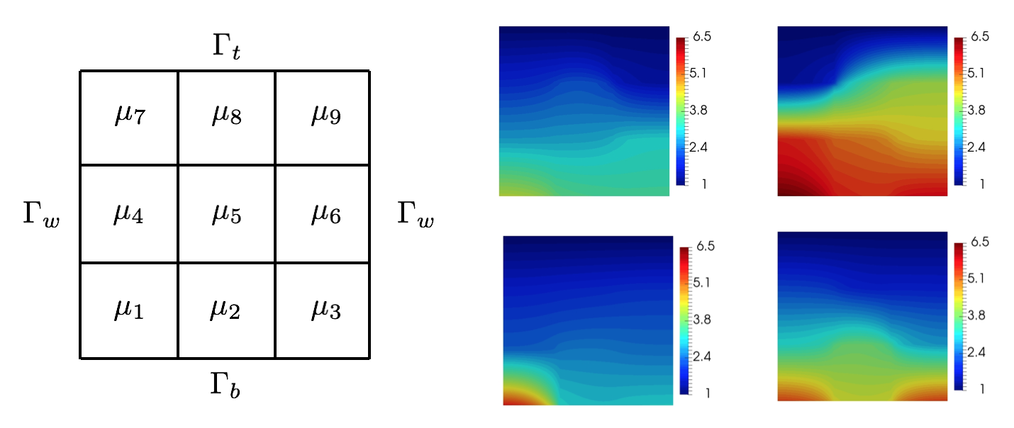
Figure 2: Test case 1. Schematic representation of the computational domain and finite-element solutions for different values of the system parameters $\boldsymbol{\mu}$.

5.1.1 ROMES model validation

We first consider statistical validation of the ROMES models, i.e., Condition 3 in Section 4.1. We set the reduced subspace dimension to $n=2$, the out-of-plane subspace dimension to $n^{\perp}=0$, and the (shared) dual-basis dimension to $n_{p}=10$. When constructing the ROMES models in Step 5 according to the description in Section 4.4, we define the set of candidate hyperparameter values $\boldsymbol{\Theta}$ via uniform full-factorial sampling in each hyperparameter dimension characterized by 12 equispaced values within the limits $\sigma^{2}\in[0.01\sigma_{t},0.25\sigma_{t}]$, $\gamma\in[0.1\sigma_{t},\sigma_{t}]$, and $0pt\in[0.001\sigma_{t},0.1\sigma_{t}]$, with $\sigma_{t}$ denoting the standard deviation of the data set $\{\hat{\delta}_{i}(\boldsymbol{\mu}))\}_{\boldsymbol{\mu}\in\mathcal{D}_{\mathrm{ROMES}}}$.

We first employ the negative log-likelihood loss function $L_{i,j}(\boldsymbol{\theta})=L_{\text{likelihood},i,j}(\boldsymbol{\theta})$ defined in Eq. (42) for hyperparameter selection. Figure 3 reports the resulting ROMES models constructed for the first error generalized coordinate using a training set with $|\mathcal{D}_{\mathrm{ROMES}}|=1000$ with two values for the dual-subspace dimension $n_{p}$. We note that for $n_{p}=4$, the data appear to be somewhat skewed and the resulting Gaussian process exhibits moderate variance. By increasing the dual-subspace dimension to $n_{p}=8$, which incurs a larger computational cost due to the increase dimension of the dual ROM equations (25), the feature becomes higher quality and thus leads to a lower-variance Gaussian process. Indeed, the ROMES model with $n_{p}=8$ appears to qualitatively capture the relationship between the error indicator and error generalized coordinate well; we now investigate this further.

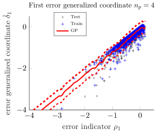
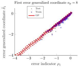
Figure 3: Test case 1. ROMES models constructed for the first two error generalized coordinates. The solid line represents the GP mean; the dashed lines represent the limits of the 99% prediction interval; the grey diamonds represent data related to online points $\boldsymbol{\mu}\in\mathcal{D}_{\mathrm{online}}$, while the blue crosses represent training data related to training points $\boldsymbol{\mu}\in\mathcal{D}_{\mathrm{ROMES}}$. We have employed $n=2$, $n^{\perp}=0$, $n_{p}=10$ and we have selected hyperparameters according to Eq. (41) with $L_{i,j}(\boldsymbol{\theta})=L_{\text{likelihood},i,j}(\boldsymbol{\theta})$, and a training set with $|\mathcal{D}_{\mathrm{ROMES}}|=1000$.

We assess the effect of the number of training-parameter instances $|\mathcal{D}_{\mathrm{ROMES}}|$ on prediction accuracy, as measured by (1) the fraction of variance unexplained (FVU)

(59) $$\text{FVU}_{i}\vcentcolon=\frac{\sum_{\boldsymbol{\mu}\in\mathcal{D}_{\mathrm{online}}}(\hat{\delta}_{i}(\boldsymbol{\mu})-\nu_{i}(\rho_{i}(\boldsymbol{\mu})))^{2}}{\sum_{\boldsymbol{\mu}\in\mathcal{D}_{\mathrm{online}}}(\hat{\delta}_{i}(\boldsymbol{\mu})-\bar{\hat{\delta}}_{i})^{2}}$$

where $\bar{\hat{\delta}}_{i}$ denotes the mean value of the error $\hat{\delta}_{i}(\boldsymbol{\mu})$ for $\boldsymbol{\mu}\in\mathcal{D}_{\mathrm{online}}$; (2) the validation frequency

(60) $$\omega_{i}(\omega)\vcentcolon=\frac{|\{\boldsymbol{\mu}\in\mathcal{D}_{\mathrm{online}}\ |\ \hat{\delta}_{i}(\boldsymbol{\mu})\in C_{i}(\omega,\boldsymbol{\mu})\}|}{|\mathcal{D}_{\mathrm{online}}|},$$

where $C_{i}(\omega,\boldsymbol{\mu})$ denotes the $\omega$-prediction interval associated with ROMES model $\tilde{\delta}_{i}$, i.e.,

(61) $$C_{i}(\omega,\boldsymbol{\mu})\vcentcolon=[\nu_{i}(\rho_{i}(\boldsymbol{\mu}))-\sqrt{2}\bar{\sigma}_{i}(\rho_{i}(\boldsymbol{\mu}))\mathrm{erf}^{-1}(\omega),\nu_{i}(\rho_{i}(\boldsymbol{\mu}))+\sqrt{2}\bar{\sigma}_{i}(\rho_{i}(\boldsymbol{\mu}))\mathrm{erf}^{-1}(\omega)],$$

where $\nu_{i}$ and $\bar{\sigma}_{i}^{2}$ denote the mean and variance associated with the $i$th ROMES model (see Eq. (47)); and (3) the Komolgorov–Smirnov (KS) statistic, which quantifies the maximum discrepancy between the cumulative distribution function (CDF) of the standard Gaussian distribution $\mathcal{N}\left(0,1\right)$ and the empirical CDF of the standardized samples of the error generalized coordinates $\{\hat{\delta}_{i}(\boldsymbol{\mu})-\nu_{i}(\rho_{i}(\boldsymbol{\mu})))/\bar{\sigma}_{i}(\rho_{i}(\boldsymbol{\mu}))\}_{\boldsymbol{\mu}\in\mathcal{D}_{\mathrm{online}}}$.

While the FVU quantifies the ability of the ROMES model $\tilde{\delta}_{i}$ to accurately model the error generalized coordinate $\hat{\delta}_{i}$ in expectation, the validation frequency and KS statistic assess the statistical properties of the model, i.e., its ability to accurately reflect the underlying data distribution. Table 1 reports these results, which show that employing $|\mathcal{D}_{\mathrm{ROMES}}|=1000$ is sufficient for the FVU to have reasonably stabilized; thus, subsequent experiments in this section set $|\mathcal{D}_{\mathrm{ROMES}}|=1000$. However, the converged prediction levels are not all correct; for example, $\omega_{1}(0.8)=0.93$ even though this value should be 0.8. We observe that one likely source of this lack of statistical validation arises from the fact that the true error does not exhibit Gaussian behavior as reported in Figure 4; indeed, these data do not pass the Shapiro–Wilk (SW) normality test, as they yield a SW statistic of $0.62$ for the first error generalized coordinate and of $0.55$ for the second. This implies that it will not be possible to achieve statistical validation in every possible metric if we employ Gaussian-process regression; rather, we may only be able to satisfy a subset of statistical-validation criteria. This motivates the need for tailored loss functions for hyperparameter selection as described in Section 4.4, as such loss functions enable the method to target specific statistical-validation criteria.

error index $i$	$1$				$2$
$|\mathcal{D}_{\mathrm{ROMES}}|$	$100$	$400$	$700$	$1000$	$100$	$400$	$700$	$1000$
FVU	0.0128	0.0133	0.0131	0.0124	0.0113	0.0115	0.0112	0.0104
$\omega_{i}(0.8)$	0.8941	0.8961	0.9127	0.9300	0.8075	0.8901	0.9167	0.9307
$\omega_{i}(0.9)$	0.9267	0.9314	0.9400	0.9534	0.8601	0.9234	0.9394	0.9500
$\omega_{i}(0.95)$	0.9414	0.9494	0.9587	0.9634	0.8894	0.9407	0.9527	0.9614
$\omega_{i}(0.99)$	0.9560	0.9680	0.9727	0.9753	0.9234	0.9614	0.9720	0.9747
KS statistic	0.2169	0.2185	0.2324	0.2504	0.0985	0.1942	0.2189	0.2348

Table 1: Test case 1. Convergence of error measures associated with the ROMES models constructed for the first two error generalized coordinates as the number of training-parameter instances $|\mathcal{D}_{\mathrm{ROMES}}|$ increases. We have employed $n=2$, $n^{\perp}=0$, $n_{p}=10$ and $|\mathcal{D}_{\mathrm{online}}|=1500$, and have selected hyperparameters according to Eq. (41) with $L_{i,j}(\boldsymbol{\theta})=L_{\text{likelihood},i,j}(\boldsymbol{\theta})$.

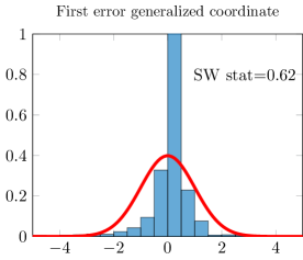
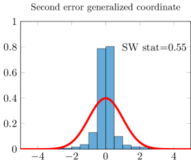
Figure 4: Test case 1. Histogram of the standardized data $\{\hat{\delta}_{i}(\boldsymbol{\mu})-\nu_{i}(\rho_{i}(\boldsymbol{\mu})))/\bar{\sigma}_{i}(\rho_{i}(\boldsymbol{\mu}))\}_{\boldsymbol{\mu}\in\mathcal{D}_{\mathrm{online}}}$, $i=1,2$ (blue bar plot) as compared to the PDF of the standard Gaussian distribution $\mathcal{N}\left(0,1\right)$ (red curve). We have employed $n=2$, $n^{\perp}=0$, $n_{p}=10$, and have selected hyperparameters according to Eq. (41) with $L_{i,j}(\boldsymbol{\theta})=L_{\text{likelihood},i,j}(\boldsymbol{\theta})$. The number of training-parameter instances is $|\mathcal{D}_{\mathrm{ROMES}}|=1000$.

To this end, we now adopt several different strategies for defining the loss function $L_{i,j}(\boldsymbol{\theta})$ employed for hyperparameter selection (see Section 4.4). In particular, we select the hyperparameters $\boldsymbol{\theta}_{i}\equiv(\sigma_{i}^{2},\gamma_{i},0pt_{i})$ characterizing the $i$th ROMES model by employing five different loss functions $L_{i,j}(\boldsymbol{\theta})$: (1) the negative log-likelihood loss $L_{\text{likelihood},i,j}$ (Eq. (42)), (2) the loss based on matching the 0.80-prediction interval $L_{0.80,i,j}$ (Eq. (43) with $\omega=0.80$), (3) the loss based on matching the 0.95-prediction interval $L_{0.95,i,j}$ (Eq. (43) with $\omega=0.95$), (4) the loss based on a linear combination of $\omega$-prediction interval losses

(62) $$L_{\text{C},i,j}\vcentcolon=\sum_{\omega\in\{0.80,0.90,0.95,0.99\}}L_{\omega,i,j},$$

and (5) the loss based on the KS statistic $L_{\text{KS},i,j}$. Table 2 reports these results for $|\mathcal{D}_{\mathrm{ROMES}}|=1000$. We note that the loss function $L_{i,j}$ employed for hyperparameter selection has a significant effect on the performance of the resulting ROMES models according to different statistical-validation criteria. In particular, the loss function can be selected to optimize improve performance with respect to particular criteria. For example, $\omega_{1}(0.8)=0.7941$ when $L_{0.80,i,j}$ is adopted, while $\omega_{1}(0.8)=0.9300$ when $L_{\text{likelihood},i,j}$ is adopted. This is an important practical result implying that the user should select the loss function to coincide with desired statistical validation criterion.

Due to its favorable performance over a range of statistical-valation criteria, we employ a loss function of $L_{i,j}=L_{\text{C},i,j}$ in the remaining experiments within Section 5.1.

error generalized coordinate index $i$	$1$
loss function $L_{i,j}(\boldsymbol{\theta})$	$L_{\text{likelihood},i,j}$	$L_{\text{C},i,j}$	$L_{0.80,i,j}$	$L_{0.95,i,j}$	$L_{\text{KS},i,j}$
FVU	0.0124	0.0126	0.0123	0.0124	0.0136
$\omega_{i}(0.8)$	0.9300	0.8361	0.7941	0.9320	0.8368
$\omega_{i}(0.9)$	0.9534	0.8854	0.8381	0.9547	0.8881
$\omega_{i}(0.95)$	0.9634	0.9194	0.8761	0.9640	0.9194
$\omega_{i}(0.99)$	0.9753	0.9507	0.9294	0.9747	0.9487
Komolgorov–Smirnov statistic	0.2504	0.2294	0.2350	0.2489	0.2288
error generalized coordinate index $i$	$2$
loss function $L_{i,j}(\boldsymbol{\theta})$	$L_{\text{likelihood},i,j}$	$L_{\text{C},i,j}$	$L_{0.80,i,j}$	$L_{0.95,i,j}$	$L_{\text{KS},i,j}$
FVU	0.0104	0.0101	0.0114	0.0111	0.0098
$\omega_{i}(0.8)$	0.9307	0.8661	0.8008	0.9427	0.7209
$\omega_{i}(0.9)$	0.9500	0.8967	0.8534	0.9594	0.7648
$\omega_{i}(0.95)$	0.9614	0.9154	0.8754	0.9700	0.7995
$\omega_{i}(0.99)$	0.9747	0.9407	0.9107	0.9767	0.8454
Komolgorov–Smirnov statistic	0.2348	0.1731	0.1196	0.2554	0.0821

Table 2: Test case 1. Statistical-validation criteria evaluated on $\mathcal{D}_{\mathrm{online}}$ (with $|\mathcal{D}_{\mathrm{online}}|=1500$) for ROMES models when different loss functions $L_{i,j}$ are employed for hyperparameter selection according to Eqs. (40) and (41) in Section 4.4. We have employed $n=2$, $n^{\perp}=0$, $n_{p}=10$ and have selected hyperparameters according to Eq. (41) with the specified loss function $L_{i,j}(\boldsymbol{\theta})$, $10$ K-fold subdivisions and a search grid made by $12^{3}$ values. The number of training-parameter instances is $|\mathcal{D}_{\mathrm{ROMES}}|=1000$.

5.1.2 In-plane and out-of-plane error approximation

We now assess the ability of the ROMES method to accurately approximate the in-plane error $\boldsymbol{\delta}^{\mathbin{\|}}$ and the out-of-plane error $\boldsymbol{\delta}^{\perp}$. To assess the ability of the method to approximate the former, we compare the mean relative ROM error

(63) $$e_{\mathbf{x}}\vcentcolon=\frac{1}{|\mathcal{D}_{\mathrm{online}}|}\sum_{\boldsymbol{\mu}\in\mathcal{D}_{\mathrm{online}}}\left(\frac{\|{\boldsymbol{\delta}}_{\mathbf{x}}(\boldsymbol{\mu})\|_{2}}{\|\mathbf{x}(\boldsymbol{\mu})\|_{2}}\right),$$

with the mean relative ROM error after applying the in-plane ROMES correction

(64) $$\tilde{e}_{\mathbf{x}}^{\mathbin{\|}}\vcentcolon=\frac{1}{|\mathcal{D}_{\mathrm{online}}|}\sum_{\boldsymbol{\mu}\in\mathcal{D}_{\mathrm{online}}}\left(\frac{\|{\boldsymbol{\delta}}_{\mathbf{x}}(\boldsymbol{\mu})-\mathbf{\Phi}\mathbb{E}[\tilde{\boldsymbol{\delta}}^{\mathbin{\|}}(\boldsymbol{\mu})]\|_{2}}{\|\mathbf{x}(\boldsymbol{\mu})\|_{2}}\right),$$

and the mean relative projection error

(65) $$e_{\mathbf{x}}^{\mathbin{\|}}\vcentcolon=\frac{1}{|\mathcal{D}_{\mathrm{online}}|}\sum_{\boldsymbol{\mu}\in\mathcal{D}_{\mathrm{online}}}\left(\frac{\|{\boldsymbol{\delta}}_{\mathbf{x}}(\boldsymbol{\mu})-\boldsymbol{\delta}^{\mathbin{\|}}(\boldsymbol{\mu})\|_{2}}{\|\mathbf{x}(\boldsymbol{\mu})\|_{2}}\right).$$

We note that the latter represents the minimum value achievable by the ROM error with the in-plane ROMES correction.

We set $n^{\perp}=0$, $L_{i,j}(\boldsymbol{\theta})=L_{\text{C},i,j}(\boldsymbol{\theta})$, and $|\mathcal{D}_{\mathrm{ROMES}}|=1000$ training-parameter instances, and we vary the reduced-subspace dimension $n$ and dual-basis dimension $n_{p}$. Figure 5 reports the results obtained for error measures $e_{\mathbf{x}}$, $\tilde{e}_{\mathbf{x}}^{\mathbin{\|}}$, and $e_{\mathbf{x}}^{\mathbin{\|}}$ over a range of values for $n$ and $n_{p}=n+i$ for $i=8,14,20$. These figures illustrate that the ROMES models for the in-plane ROMES correction $\tilde{\boldsymbol{\delta}}^{\mathbin{\|}}$ enable the mean state error to be significantly reduced with respect to the ROM error, as $\tilde{e}_{\mathbf{x}}^{\mathbin{\|}}$ is smaller than $e_{\mathbf{x}}$ in all cases; moreover, the mean relative ROM error after applying the in-plane ROMES correction state error $\tilde{e}_{\mathbf{x}}^{\mathbin{\|}}$ approaches the optimal value defined by the mean relative projection error $e_{\mathbf{x}}^{\mathbin{\|}}$ as the dual-basis dimension $n_{p}$ increases. Indeed, because equality in (26) holds when the ROM approximation of the duals is exact (i.e., $\mathbf{p}_{i}\approx\tilde{\mathbf{p}}_{i}$) and the residual is linear in its first argument (i.e., Eq. (2) holds)—the latter of which is true for this problem—we expect the ROMES models to be extremely accurate for this problem as the dimension of the dual reduced basis $n_{p}$ becomes large. Thus, we conclude that the proposed approach is indeed able to accurately approximate the in-plane error. That is, the proposed method constructs an accurate statistical closure model.

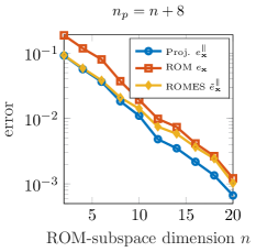
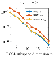
Figure 5: Test case 1. Mean relative ROM error $e_{\mathbf{x}}$ (red), mean relative ROM error after applying the in-plane ROMES correction $\tilde{e}_{\mathbf{x}}^{\mathbin{\|}}$ (yellow), and mean relative projection error $e_{\mathbf{x}}^{\mathbin{\|}}$ (blue) for a varying reduced-subspace dimension $n$ and dual-subspace dimension $n_{p}$. Here, we set $n^{\perp}=0$, $L_{i,j}(\boldsymbol{\theta})=L_{\text{C},i,j}(\boldsymbol{\theta})$, $|\mathcal{D}_{\mathrm{ROMES}}|=1000$ and $|\mathcal{D}_{\mathrm{online}}|=1500$.

We perform a similar analysis for the out-of-plane error by comparing the mean relative ROM error $e_{\mathbf{x}}$ with the mean relative ROM error after applying both the in-plane and out-of-plane ROMES corrections

(66) $$\tilde{e}_{\mathbf{x}}^{\mathbin{\|}+\perp}\vcentcolon=\frac{1}{|\mathcal{D}_{\mathrm{online}}|}\sum_{\boldsymbol{\mu}\in\mathcal{D}_{\mathrm{online}}}\left(\frac{\|{\boldsymbol{\delta}}_{\mathbf{x}}(\boldsymbol{\mu})-\mathbf{\Phi}\mathbb{E}[\tilde{\boldsymbol{\delta}}^{\mathbin{\|}}(\boldsymbol{\mu})]-\mathbf{\Phi}^{\perp}\mathbb{E}[\tilde{\boldsymbol{\delta}}^{\perp}(\boldsymbol{\mu})]\|_{2}}{\|\mathbf{x}(\boldsymbol{\mu})\|_{2}}\right)$$

and the mean relative projection error

(67) $$e_{\mathbf{x}}^{\mathbin{\|}+\perp}\vcentcolon=\frac{1}{|\mathcal{D}_{\mathrm{online}}|}\sum_{\boldsymbol{\mu}\in\mathcal{D}_{\mathrm{online}}}\left(\frac{\|{\boldsymbol{\delta}}_{\mathbf{x}}(\boldsymbol{\mu})-\boldsymbol{\delta}^{\mathbin{\|}}(\boldsymbol{\mu})-\boldsymbol{\delta}^{\perp}(\boldsymbol{\mu})\|_{2}}{\|\mathbf{x}(\boldsymbol{\mu})\|_{2}}\right),$$

which represents the minimum value achievable by the ROM error with both in-plane and out-of-plane ROMES correction. Figure 6 reports the results obtained for error measures $e_{\mathbf{x}}$, $\tilde{e}_{\mathbf{x}}^{\mathbin{\|}+\perp}$, and $e_{\mathbf{x}}^{\mathbin{\|}+\perp}$ for various values of the reduced-subspace dimension $n$, the dual-basis dimension $n_{p}$, and the out-of-plane subspace dimension $n^{\perp}$. We again observe that the ROMES corrections enable significant error reduction, and performance improves as the dual-basis dimension $n_{p}$ increases. Thus, we conclude that the proposed approach is able to accurately approximate both the in-plane and out-of-plane errors.

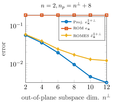
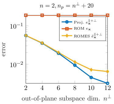
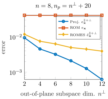
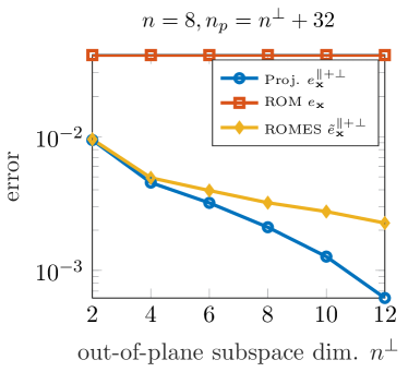
Figure 6: Test case 1. Mean relative ROM error $e_{\mathbf{x}}$ (red), mean relative ROM error after applying the in-plane and out-of-plane ROMES corrections $\tilde{e}_{\mathbf{x}}^{\mathbin{\|}+\perp}$ (yellow), and mean relative projection error $e_{\mathbf{x}}^{\mathbin{\|}+\perp}$ (blue) for a varying reduced-subspace dimension $n$, dual-subspace dimension $n_{p}$, and out-of-plane subspace dimension $n^{\perp}$. Here, we set $L_{i,j}(\boldsymbol{\theta})=L_{\text{C},i,j}(\boldsymbol{\theta})$, $|\mathcal{D}_{\mathrm{ROMES}}|=1000$, and $|\mathcal{D}_{\mathrm{online}}|=1500$.

5.1.3 Quantity-of-interest error approximation

We now consider the ability of the proposed ROMES models to construct statistical models of quantities of interest $\mathbf{\tilde{q}}$ as proposed in Section 4.5. To this end, we consider $s=2$ quantities of interest

(68) $$\mathbf{q}:\boldsymbol{\nu}\mapsto\mathbf{s}(\mathbf{x}(\boldsymbol{\nu});\boldsymbol{\nu})=\begin{bmatrix}\boldsymbol{\gamma}^{T}\mathbf{x}(\boldsymbol{\nu})\\ \mathbf{x}(\boldsymbol{\nu})^{T}\mathbf{M}\mathbf{x}(\boldsymbol{\nu})\end{bmatrix},$$

where ${q}_{1}$ and ${q}_{2}$ represent the mean value (i.e., $\int_{\Omega_{\vec{x},5}}u\mathrm{d}\vec{x}=\boldsymbol{\gamma}^{T}\mathbf{x}$) and the mean squared value (i.e., $\int_{\Omega_{\vec{x},5}}u^{2}\mathrm{d}\vec{x}=\mathbf{x}^{T}\mathbf{M}\mathbf{x}$) of the state variable over $\Omega_{\vec{x},5}$, respectively. We emphasize that these quantities of interest were not specified during the offline stage (see Remark 4.2).

We set the loss function to $L_{i,j}(\boldsymbol{\theta})=L_{\text{C},i,j}(\boldsymbol{\theta})$ and number of training-parameter instances to $|\mathcal{D}_{\mathrm{ROMES}}|=1000$. Figures 7 and 8 plot the FOM-computed quantity of interest ${q}_{i}(\boldsymbol{\mu})$ versus both the ROM-computed quantity of interest $q_{\mathrm{ROM},i}(\boldsymbol{\mu})$ and the expected value of the ROMES-corrected quantity of interest $\mathbb{E}[{\tilde{q}}_{i}(\boldsymbol{\mu})]$, $i=1,2$ for several values of the reduced-subspace dimensions $n$ and $n^{\perp}$ and for $\boldsymbol{\mu}\in\mathcal{D}_{\mathrm{online}}$.

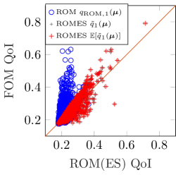
(a) $n=2$, $n^{\perp}=0$

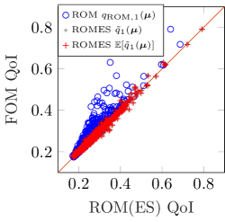
(b) $n=6$, $n^{\perp}=0$

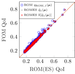
(c) $n=10$, $n^{\perp}=0$

(d) $n=2$, $n^{\perp}=2$

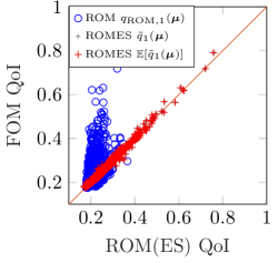
(e) $n=2$, $n^{\perp}=6$

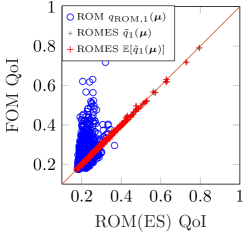
(f) $n=2$, $n^{\perp}=10$

Figure 7: Test case 1. Scatter plot of the FOM-computed (linear) quantity of interest ${q}_{1}(\boldsymbol{\mu})$ versus both the ROM-computed quantity of interest $q_{\mathrm{ROM},1}(\boldsymbol{\mu})$ (blue circles) and the expected value of the ROMES-corrected quantity of interest $\mathbb{E}[{\tilde{q}}_{1}(\boldsymbol{\mu})]$ (red crosses) for several values of the reduced-subspace dimension $n$ and for $\boldsymbol{\mu}\in\mathcal{D}_{\mathrm{online}}$. They grey crosses are computed by taking the maximum and the minimum value of the $\tilde{q}_{1}(\boldsymbol{\mu})$ over $100$ realizations of the ROMES statistical model. Here, we set $L_{i,j}(\boldsymbol{\theta})=L_{\text{C},i,j}(\boldsymbol{\theta})$, $|\mathcal{D}_{\mathrm{ROMES}}|=1000$, and $n_{p}=10$.

Figure 9 reports the associated FVU values, with the FVU defined as

(69) $$\text{FVU}_{{q}_{i}}(q)\vcentcolon=\frac{\sum_{\boldsymbol{\mu}\in\mathcal{D}_{\mathrm{online}}}({q}_{i}(\boldsymbol{\mu})-q(\boldsymbol{\mu}))^{2}}{\sum_{\boldsymbol{\mu}\in\mathcal{D}_{\mathrm{online}}}({q}_{i}(\boldsymbol{\mu})-{\bar{q}}_{i})^{2}},$$

where ${\bar{q}}_{i}$ denotes the mean value of the quantity of interest ${q}_{i}(\boldsymbol{\mu})$ for $\boldsymbol{\mu}\in\mathcal{D}_{\mathrm{online}}$. These plots demonstrate that the proposed method significantly reduces the quantity-of-interest error without the need for prescribing the quantities of interest in the offline stage (see Remark 4.2), and performance is improved as the dual-basis dimension $n_{p}$ increases.

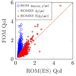
(a) $n=2$, $n^{\perp}=0$

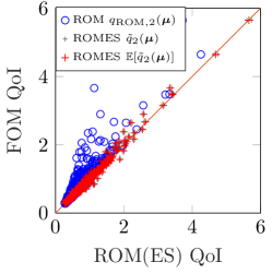
(b) $n=6$, $n^{\perp}=0$

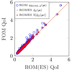
(c) $n=10$, $n^{\perp}=0$

(d) $n=2$, $n^{\perp}=2$

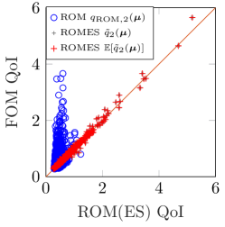
(e) $n=2$, $n^{\perp}=6$

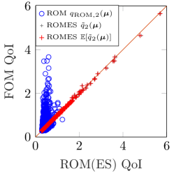
(f) $n=2$, $n^{\perp}=10$

Figure 8: Test case 1. Scatter plot of the FOM-computed (nonlinear) quantity of interest ${q}_{2}(\boldsymbol{\mu})$ versus both the ROM-computed quantity of interest $q_{\mathrm{ROM},2}(\boldsymbol{\mu})$ (blue circles) and the expected value of the ROMES-corrected quantity of interest $\mathbb{E}[{\tilde{q}}_{2}(\boldsymbol{\mu})]$ (red crosses) for several values of the reduced-subspace dimension $n$ and for $\boldsymbol{\mu}\in\mathcal{D}_{\mathrm{online}}$. They grey crosses are computed by taking the maximum and the minimum value of the $\tilde{q}_{2}(\boldsymbol{\mu})$ over $100$ realizations of the ROMES statistical model. Here, we set $L_{i,j}(\boldsymbol{\theta})=L_{\text{C},i,j}(\boldsymbol{\theta})$, $|\mathcal{D}_{\mathrm{ROMES}}|=1000$, and $n_{p}=10$.

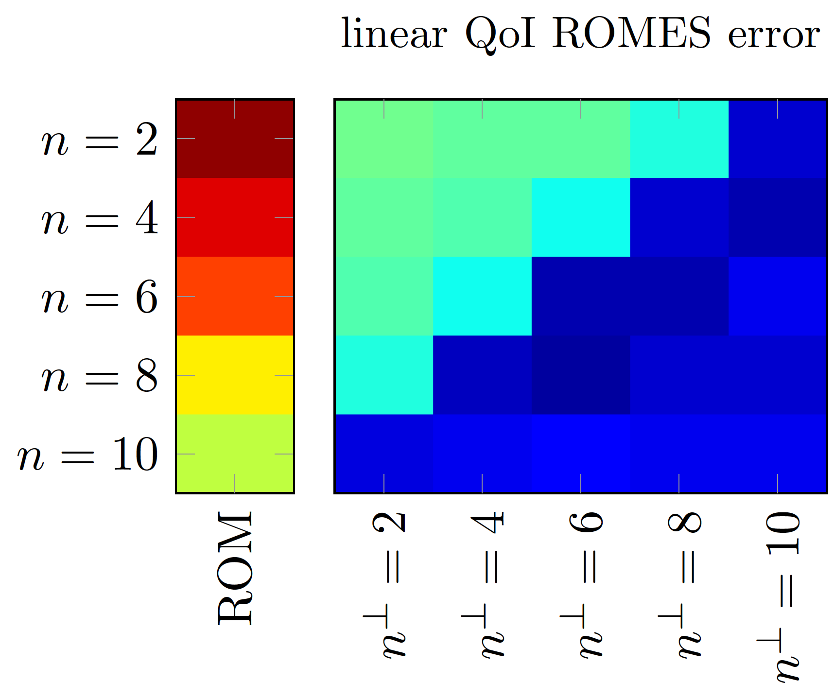
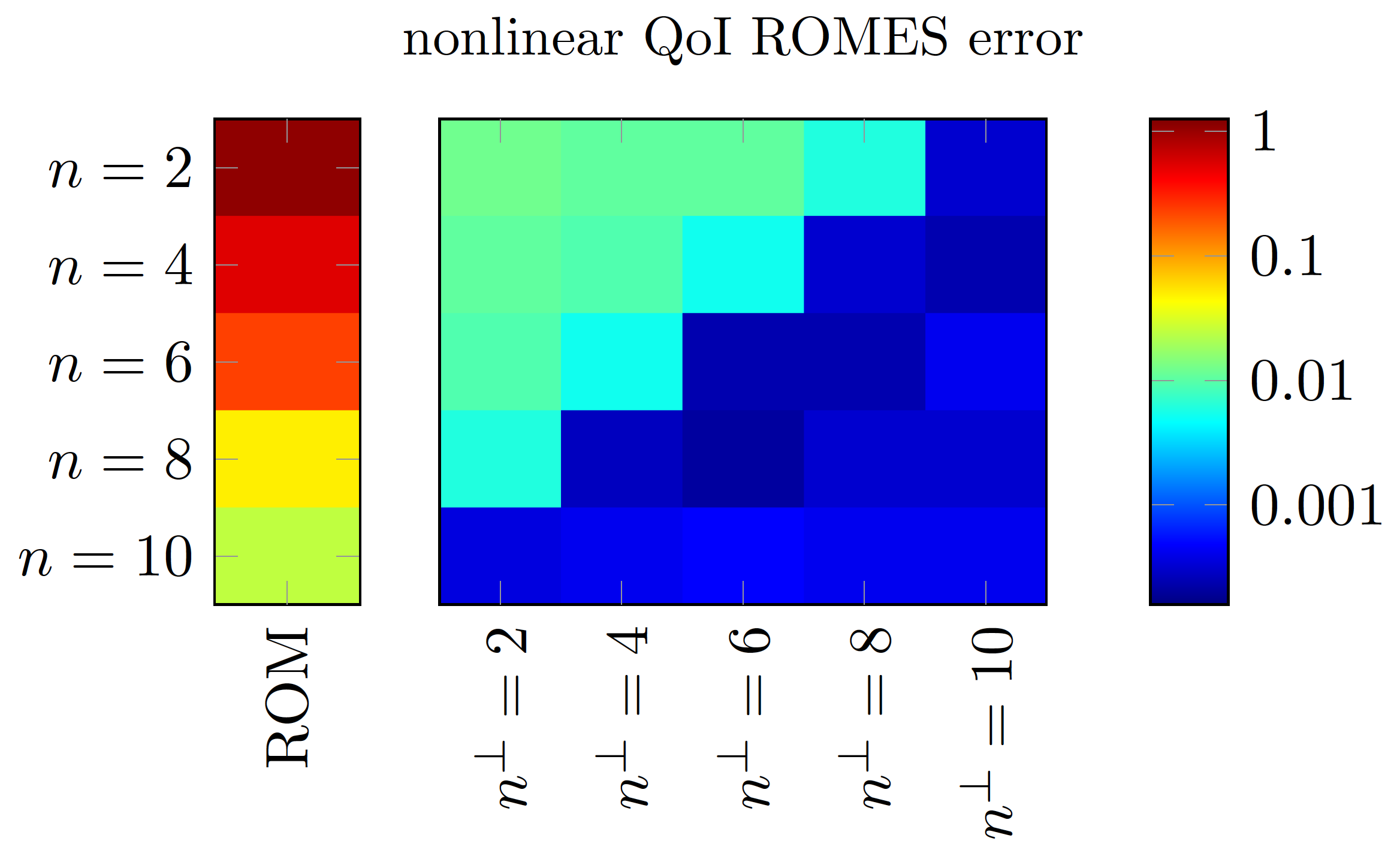
Figure 9: Test case 1. FVU values associated with the ROM-computed quantities of interest $q_{\mathrm{ROM},1}$ and $q_{\mathrm{ROM},2}$ and the expected value of the ROMES-corrected quantity of interest $\mathbb{E}[{\tilde{q}}_{1}]$ and $\mathbb{E}[{\tilde{q}}_{2}]$ for several values of the reduced-subspace dimension $n$ and $n^{\perp}$. Here, we set $L_{i,j}(\boldsymbol{\theta})=L_{\text{C},i,j}(\boldsymbol{\theta})$, $|\mathcal{D}_{\mathrm{ROMES}}|=1000$, and $n_{p}=32$.

5.1.4 Computational efficiency

The previous results in this section illustrate the ability of the proposed method to reduce errors with respect to a ‘ROM-only’ approach (i.e., a method that executes only Step 1 in Algorithm 2). However, the method achieves this at an increased online cost, as it additionally executes Steps 2–5 in Algorithm 2; the dominant additional cost arises from the need to compute the approximate dual solutoins in Step 2 (see Remark 4.3). However, we note that regardless of computational cost, the proposed method yields a statistical model of the full-order model state and quantity of interest, while a ROM-only approach does not. Thus, even with increased cost, the proposed method is more amenable to integration within uncertainty-quantification applications. Nonetheless, we now perform an assessment of the computational efficiency of a ‘ROM-only’ approach and the proposed method.

To perform this assessment, we subject the ‘ROM-only’ method, the proposed method with a ROMES in-plane correction only, and the proposed method with both an in-plane and out-of-plane correction to a wide range of parameter values. In particular, we consider all combinations of $n\in\{1,\ldots,20\}$, $n_{p}\in\{n,\ldots,n+15\}$ (not relevant to the ‘ROM-only’ method), and $n^{\perp}\in\{1,\ldots,15\}$ (not relevant to the ‘ROM-only’ method or the proposed method with in-plane correction only). Figure 10 reports these results. For each value of these parameters, we compute both the relative error and the wall time for the simulations relative to that incurred by the full-order model (as averaged over all online points $\boldsymbol{\mu}\in\mathcal{D}_{\mathrm{online}}$). The relative errors for the ROM-only approach, the proposed method with a ROMES in-plane correction only, and the proposed method with both an in-plane and out-of-plane correction correspond to $e_{\mathbf{x}}$ (Eq. (63)), $\tilde{e}_{\mathbf{x}}^{\mathbin{\|}}$ (Eq. (64)), and $\tilde{e}_{\mathbf{x}}^{\mathbin{\|}+\perp}$ (Eq. (66)), respectively. The figure reports a Pareto front for each method, which is characterized by the method parameters that minimize the competing objectives of relative error and relative wall time.

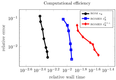
Figure 10: Test case 1. Computational efficiency of the ‘ROM-only’ approach (ROM $e_{\mathbf{x}}$), the proposed method with a ROMES in-plane correction only (ROMES $\tilde{e}_{\mathbf{x}}^{\mathbin{\|}}$), and the proposed method with both an in-plane and out-of-plane correction (ROMES $\tilde{e}_{\mathbf{x}}^{\mathbin{\|}+\perp}$) over a range of method parameters, and associated Pareto fronts. Here, the relative wall time is reported relateve to that incurred by the full-order model. Note that the ROM-only approach is Pareto dominant due to the fact that the residual is linear in its first argument for this problem (i.e., Eq. (2) holds).

These results show that the ‘ROM-only’ approach is Pareto dominant, which is likely due to the fact that the residual is linear in its first argument for this problem (i.e., Eq. (2) holds). Because of this, the cost of the dual ROM solves in Step 2 of Algorithm 2 is similar to that of the (primal) ROM solve executed in Step 1 of Algorithm 2. Thus, in this case, it is always computationally more efficient to employ a larger ROM dimension $n$ than to approximate the errors according to the proposed technique if we are only interested in minimizing the FVU. As described in Section 4.5, we expect the proposed method to be most effective when the ROM equations are nonlinear, as the dual problems remain linear in this case, thus allowing Steps 2–5 to be computationally inexpensive relative to Step 1. The next set of experiments will highlight this fact.

Nonetheless, we again emphasize that the ‘ROM-only’ approach does not generate a statistical model of the FOM state or the FOM quantity of interest, while the proposed approach does provide this. Thus, even in the linear case, the proposed method may still be considered more amenable to integration with uncertainty quantification than the ‘ROM-only’ approach, as the proposed method provides a mechanism to quantify the ROM-induced uncertainty.

5.2 Test case 2: nonlinear mechanical response

We now assess the proposed method on a problem characterized by a residual that is nonlinear in its first argument. In particular, we consider a static, nonlinear mechanical-response problem in three spatial dimensions. We consider a Saint Venant–Kirchhoff material, whose strain-energy function is given by

$${W}(\mathbf{E})=\frac{\lambda_{1}}{2}\mathrm{tr}(\mathbf{E})^{2}+\lambda_{2}\mathrm{tr}(\mathbf{E}^{2}),$$

where $\mathbf{E}\in\mathbb{R}^{3\times 3}$ denotes the Lagrangian Green strain tensor and $\lambda_{1}$ and $\lambda_{2}$ denote Lamé constants

$$\lambda_{1}=\frac{\nu E}{(1+\nu)(1-2\nu)}\qquad\text{and}\qquad\lambda_{2}=\frac{E}{2(1+\nu)}.$$

Defining the deformation gradient tensor as $\mathbf{F}=\mathbf{I}+\nabla\mathbf{u}\in\mathbb{R}^{3\times 3}$, where $\mathbf{u}=\mathbf{u}(\vec{x};\boldsymbol{\mu})\in\mathbb{R}^{3}$ denotes the deformation, we obtain the Piola tensor

$$\mathbf{P}=\lambda_{1}\mathrm{tr}(\mathbf{E})\mathbf{F}+2\lambda_{2}\mathbf{F}\mathbf{E}.$$

The shear test on the domain $\Omega_{\vec{x},0}=[0,1]^{3}$ reads as follows: find $\mathbf{u}$ satisfying

(70) $$\begin{cases}\text{div}(\mathbf{P}(\mathbf{u};\boldsymbol{\mu}))=\bf{0}&\vec{x}\in\Omega_{\vec{x},0}\\ \mathbf{P}(\mathbf{u};\boldsymbol{\mu})\mathbf{n}(\vec{x})=\mu_{3}\mathbf{n}_{z}&\vec{x}\in\Gamma_{N}\\ \mathbf{P}(\mathbf{u};\boldsymbol{\mu})\mathbf{n}(\vec{x})=\bf{0}&\vec{x}\in\Gamma_{N,\mathrm{free}}\\ \mathbf{u}=\bf{0}&\vec{x}\in\Gamma_{D},\end{cases}$$

where $\mathbf{n}(\vec{x})\equiv[n_{x}(\vec{x}),n_{y}(\vec{x}),n_{z}(\vec{x})]$ denotes the outward unit normal. We consider ${d}=3$ parameters comprising the Young’s modulus $\mu_{1}=E\in[6\times 10^{4},8\times 10^{4}]$, the Poisson coefficient $\mu_{2}=\nu\in[0.3,0.45]$, and the external-load magnitude $\mu_{3}\in[1\times 10^{3},2.5\times 10^{3}]$.

                 

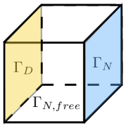
Figure 11: Test case 2. Geometry and boundary faces (left) and reduced meshes for DEIM approximation of residual vectors (center) and MDEIM approximation of Jacobian matrices.

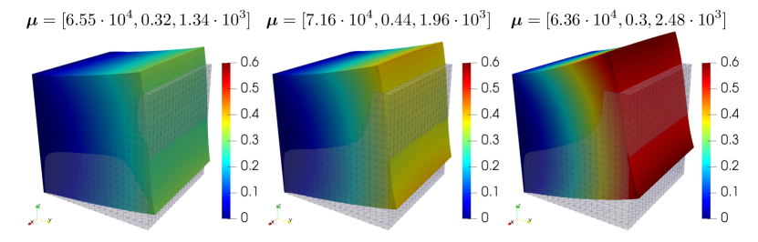
Figure 12: Test case 2. Finite element approximation of problem (70) for three different values of the parameter vector $\boldsymbol{\mu}$.

We discretize the spatial domain using the finite-element method on a conformal computational mesh given by $41154$ tetrahedra and linear finite elements. This yields FOM governing equations of the form (1) with ${N}=8000$ degrees of freedom with the residual $\mathbf{r}$ nonlinear in its first argument.

We execute the offline stage using Algorithm 1 as follows. We construct the training-parameter sets by drawing uniform random samples from the parameter domain $\mathcal{D}$. We set $|\mathcal{D}_{\mathrm{dual}}|=10$, while $|\mathcal{D}_{\mathrm{ROMES}}|$ varies across experiments. In Step 1, we apply POD to FOM solutions computed at parameter instances $\mathcal{D}_{\mathrm{POD}}$ with $|\mathcal{D}_{\mathrm{POD}}|=10$. We employ Galerkin projection such that $\mathbf{\Psi}=\mathbf{\Phi}$; the reduced-subspace dimension $n$ varies across experiments. Because the residual is nonlinear in its first argument, we require a hyper-reduction method to ensure that solving the ROM equations incurs an ${N}$-independent computational complexity. For this purpose, we apply the DEIM method [4, 12] to approximate the nonlinear component of the residual, which comprises the sum of a nonlinear component and a linear component (the boundary conditions). For each value of the reduced dimension $n$, we collect snapshots of this nonlinear component evaluated at the ROM solution (without hyper-reduction) at 30 parameter instances (which includes $\mathcal{D}_{\mathrm{POD}}$), and we truncate the POD basis such that it preserves $1-1\times 10^{-8}$ of the relative statistical energy. Step 2 constructs the basis matrix $\mathbf{\Phi}^{\perp}$ from the discarded POD modes; the out-of-plane subspace dimension $n^{\perp}$ also depends on the particular experiment. In Step 3, we construct a single shared trial dual basis matrix $\mathbf{\Phi}_{p}$ (i.e., $\mathbf{\Phi}_{p,{i}}=\mathbf{\Phi}_{p}$, $i=1,\ldots,{\bar{n}}$) by combining snapshots from from all ${\bar{n}}$ dual solves executed at parameter instances $\boldsymbol{\mu}\in\mathcal{D}_{\mathrm{dual}}$ (see Remark 3.3 in Section 3.4). We also employ Galerkin projection for the dual problem such that $\mathbf{\Psi}_{p,{i}}=\mathbf{\Psi}_{p}=\mathbf{\Phi}_{p}$, $i=1,\ldots,{\bar{n}}$; the dual-basis dimension $n_{p}$ also varies across experiments. Because the system matrix in the dual ROM equations (25) exhibits non-affine parameter dependence (but the right-hand side is linear and parameter-independent), we apply MDEIM [32] to approximate the system matrix; because the right-hand side is linear and parameter-independent, it does not require hyper-reduction. For MDEIM, we collect snapshots of the system matrix in an identical way to the DEIM snapshot-collection procedure described above, and we use the same truncation criterion.

For the online stage, we execute Algorithm 2 for all parameter instances in $\mathcal{D}_{\mathrm{online}}$, which comprises $|\mathcal{D}_{\mathrm{online}}|=1000$ values drawn uniformly at random from $\mathcal{D}$. The remaining inputs to Algorithm 2 result from the outputs of Algorithm 1. Note that we use DEIM when dealing with the ROM equations (4) in Step 1 and MDEIM when assembling the dual ROM equations (25) in Step 2.

5.2.1 ROMES model validation

As in Section 5.1.1, we first consider statistical validation of the ROMES models, i.e., condition 3 in Section 4.1. When constructing the Gaussian processes in Step 5 according to the description in Section 4.4, we define the set of candidate hyperparameter values $\boldsymbol{\Theta}$ as uniform full-factorial sampling in each hyperparameter dimension characterized by 10 equispaced values within the limits $\sigma^{2}\in[0.01\sigma_{t},0.25\sigma_{t}]$, $\gamma\in[0.1\sigma_{t},\sigma_{t}]$, and $0pt\in[0.001\sigma_{t},0.1\sigma_{t}]$, with $\sigma_{t}$ denoting the standard deviation of the data $\{\hat{\delta}_{i}(\boldsymbol{\mu}))\}_{\boldsymbol{\mu}\in\mathcal{D}_{\mathrm{ROMES}}}$.

We first consider using the negative log-likelihood loss function $L_{i,j}(\boldsymbol{\theta})=L_{\text{likelihood},i,j}(\boldsymbol{\theta})$ defined in Eq. (42) for hyperparameter selection. Figure 13 reports the resulting ROMES models constructed for the first error generalized coordinate using a training set $|\mathcal{D}_{\mathrm{ROMES}}|=400$ with two values for the dual-subspace dimension $n_{p}$. We note that for $n_{p}=4$, the data appear to be skewed and the resulting Gaussian process exhibits large variance. By increasing the dual-subspace dimension to $n_{p}=12$, the feature becomes higher quality and thus leads to a lower-variance Gaussian process that qualitatively captures the relationship between the error indicator and error generalized coordinate well. We now investigate this further.

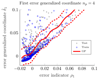
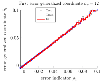
Figure 13: Test case 2. ROMES models constructed for the first error generalized coordinate with different dual-subspace dimensions $n_{p}$. The solid line represents the GP mean; the dashed lines represent the limits of the 99% prediction interval; the grey crosses represent data related to prediction points $\boldsymbol{\mu}\in\mathcal{D}_{\mathrm{online}}$, while the blue crosses represent training data related to prediction points $\boldsymbol{\mu}\in\mathcal{D}_{\mathrm{ROMES}}$. We have employed $n=3$, $n^{\perp}=0$, and we have selected hyperparameters according to Eq. (41) with $L_{i,j}(\boldsymbol{\theta})=L_{\text{likelihood},i,j}(\boldsymbol{\theta})$, and a training set with $|\mathcal{D}_{\mathrm{ROMES}}|=400$.

We assess the effect of the number of training-parameter instances $|\mathcal{D}_{\mathrm{ROMES}}|$ on prediction accuracy, as measured by the fraction of variance unexplained (FVU) $\text{FVU}_{i}$ defined in Eq. (59), the validation frequency $\omega_{i}(\omega)$ defined in Eq. (60), and the Komolgorov–Smirnov (KS) statistic, which quantifies the maximum discrepancy between the CDR of $\mathcal{N}\left(0,1\right)$ and the empirical CDF of the standardized samples $\{\hat{\delta}_{i}(\boldsymbol{\mu})-\nu_{i}(\rho_{i}(\boldsymbol{\mu})))/\bar{\sigma}_{i}(\rho_{i}(\boldsymbol{\mu}))\}_{\boldsymbol{\mu}\in\mathcal{D}_{\mathrm{online}}}$.

Table 3 reports these results, which show that employing $|\mathcal{D}_{\mathrm{ROMES}}|=400$ is sufficient for the test FVU to have reasonably stabilized; thus, subsequent experiments in this section set $|\mathcal{D}_{\mathrm{ROMES}}|=400$. As observed in Section 5.1.1, the converged values of FVU are quite small, but the converged prediction levels are not all correct. For example, $\omega_{1}(0.8)=0.9200$ even though this value should be 0.8. This again occurs because the data are not Gaussian; Figure 14 shows this. In fact, the data do not pass Shapiro–Wilk normality test, as they yield values of f $0.41$ for the first error generalized coordinate and of $0.46$ for the second, which again implies that it will not be possible to achieve statistical validation in every possible metric if we employ Gaussian-process regression. This motivates the need for tailored loss functions as described in Section 4.4.

error index $i$	$1$				$2$
$|\mathcal{D}_{\mathrm{ROMES}}|$	$100$	$200$	$300$	$400$	$100$	$200$	$300$	$400$
FVU	0.0035	0.0036	0.0031	0.0028	0.0025	0.0032	0.0011	0.0008
$\omega_{i}(0.8)$	0.8983	0.9167	0.9233	0.9200	0.9217	0.8917	0.9183	0.9117
$\omega_{i}(0.9)$	0.9150	0.9200	0.9317	0.9283	0.9300	0.9033	0.9350	0.9233
$\omega_{i}(0.95)$	0.9250	0.9300	0.9383	0.9417	0.9333	0.9117	0.9467	0.9317
$\omega_{i}(0.99)$	0.9467	0.9450	0.9450	0.9500	0.9567	0.9367	0.9567	0.9483
KS statistic	0.2030	0.2822	0.2804	0.2388	0.2781	0.3123	0.3439	0.3438

Table 3: Test case 2. Convergence of error measures associated with the ROMES models constructed for the first two error generalized coordinates as the number of training-parameter instances $|\mathcal{D}_{\mathrm{online}}|$ increases. We have employed $n=2$, $n^{\perp}=0$, $n_{p}=12$, $|\mathcal{D}_{\mathrm{online}}|=600$ and , and have selected hyperparameters according to Eq. (41) with $L_{i,j}(\boldsymbol{\theta})=L_{\text{likelihood},i,j}(\boldsymbol{\theta})$.

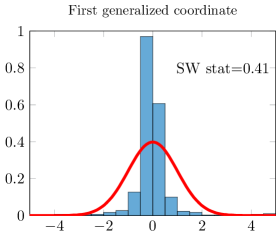
Figure 14: Test case 2. Histogram of the standardized data $\{\hat{\delta}_{i}(\boldsymbol{\mu})-\nu_{i}(\rho_{i}(\boldsymbol{\mu})))/\bar{\sigma}_{i}(\rho_{i}(\boldsymbol{\mu}))\}_{\boldsymbol{\mu}\in\mathcal{D}_{\mathrm{online}}}$, $i=1,2$ (blue bar plot) as compared to the PDF of the standard Gaussian distribution $\mathcal{N}\left(0,1\right)$ (red curve). We have employed $n=3$, $n^{\perp}=0$, $n_{p}=10$, and have selected hyperparameters according to Eq. (41) with $L_{i,j}(\boldsymbol{\theta})=L_{\text{likelihood},i,j}(\boldsymbol{\theta})$. The number of training-parameter instances is $|\mathcal{D}_{\mathrm{ROMES}}|=400$.

As in Section 5.1.1, we consider five different loss functions $L_{i,j}(\boldsymbol{\theta})$ for hyperparameter selection (see Section 4.4): (1) the negative log-likelihood loss $L_{\text{likelihood},i,j}$ (Eq. (42)), (2) the loss based on matching the 0.80-prediction interval $L_{0.80,i,j}$ (Eq. (43) with $\omega=0.80$), (3) the loss based on matching the 0.95-prediction interval $L_{0.95,i,j}$ (Eq. (43) with $\omega=0.95$), (4) the loss based on a linear combination of $\omega$-prediction interval losses $L_{\text{C},i,j}$ (Eq. (62)), and (5) the loss based on the KS statistic $L_{\text{KS},i,j}$.

Table 4 reports these results for $|\mathcal{D}_{\mathrm{ROMES}}|=1000$. As in Section 5.1.1, we observe that the loss function $L_{i,j}$ has a significant effect on the performance of the resulting ROMES models according to different statistical-validation criteria, and can be chosen to target performence with respect to particular criteria: $\omega_{1}(0.8)=0.81$ instead of $\omega_{1}(0.8)=0.92$ and $\omega_{1}(0.8)=0.8250$ instead of $\omega_{1}(0.8)=0.9117$ when $L_{0.80,i,j}$ is adopted.

We again employ a loss function of $L_{i,j}=L_{\text{C},i,j}$ in the remaining experiments within this section due to its favorable performance over a range of statistical-valation criteria.

error generalized coordinate index $i$	$1$
loss function $L_{i,j}(\boldsymbol{\theta})$	$L_{\text{likelihood},i,j}$	$L_{\text{C},i,j}$	$L_{0.80,i,j}$	$L_{0.95,i,j}$	$L_{\text{KS},i,j}$
FVU	0.0028	0.0029	0.0015	0.0017	0.0015
$\omega_{i}(0.8)$	0.9200	0.8750	0.8100	0.9183	0.8133
$\omega_{i}(0.9)$	0.9283	0.9117	0.8567	0.9400	0.8567
$\omega_{i}(0.95)$	0.9417	0.9217	0.8733	0.9483	0.8767
$\omega_{i}(0.99)$	0.9500	0.9317	0.8950	0.9567	0.8900
Komolgorov–Smirnov statistic	0.2388	0.1816	0.1179	0.3280	0.0908
error generalized coordinate index $i$	$2$
loss function $L_{i,j}(\boldsymbol{\theta})$	$L_{\text{likelihood},i,j}$	$L_{\text{C},i,j}$	$L_{0.80,i,j}$	$L_{0.95,i,j}$	$L_{\text{KS},i,j}$
FVU	0.00082	0.00081	0.00075	0.00076	0.00076
$\omega_{i}(0.8)$	0.9117	0.8617	0.8250	0.9167	0.8133
$\omega_{i}(0.9)$	0.9233	0.8817	0.8533	0.9383	0.8383
$\omega_{i}(0.95)$	0.9317	0.8983	0.8667	0.9500	0.8633
$\omega_{i}(0.99)$	0.9483	0.9100	0.8950	0.9667	0.8867
Komolgorov–Smirnov statistic	0.3438	0.2467	0.1329	0.3120	0.1135

Table 4: Test case 2. Statistical-validation criteria for ROMES models when different loss functions $L_{i,j}$ are employed for hyperparameter selection according to Eqs. (40) and (41) in Section 4.4. We have employed $n=2$, $n^{\perp}=0$, $n_{p}=10$, and have selected hyperparameters according to Eq. (41) with the specified loss function $L_{i,j}(\boldsymbol{\theta})$. The number of training-parameter instances is $|\mathcal{D}_{\mathrm{ROMES}}|=400$, while $|\mathcal{D}_{\mathrm{online}}|=600$.

5.2.2 In-plane and out-of-plane error approximation

As in Section 5.1.2, we now assess the ability of the proposed method to accurately approximate the in-plane error $\boldsymbol{\delta}^{\mathbin{\|}}$ and the out-of-plane error $\boldsymbol{\delta}^{\perp}$. In particular, we compare the mean relative ROM error $e_{\mathbf{x}}$ (Eq. (63)) with the mean relative ROM error after applying the in-plane ROMES correction $\tilde{e}_{\mathbf{x}}^{\mathbin{\|}}$ (Eq. (64)) and the mean relative projection error $e_{\mathbf{x}}^{\mathbin{\|}}$ (Eq. (65)).

Figure 15 reports the results obtained for $n^{\perp}=0$, $L_{i,j}(\boldsymbol{\theta})=L_{\text{C},i,j}(\boldsymbol{\theta})$, and $|\mathcal{D}_{\mathrm{ROMES}}|=400$ training-parameter instances, and a range of values for $n$ and $n_{p}$. We first note that the mean relative ROM error $e_{\mathbf{x}}$ is relatively close to the (optimal) mean relative projection error $e_{\mathbf{x}}^{\mathbin{\|}}$, implying that the in-plane error is quite small for this particular problem; however the proposed method is indeed able to bridge this gap, as the in-plane ROMES correction $\tilde{\boldsymbol{\delta}}^{\mathbin{\|}}$ enables $\tilde{e}_{\mathbf{x}}^{\mathbin{\|}}$ to be nearly equal to the optimal value $e_{\mathbf{x}}^{\mathbin{\|}}$.

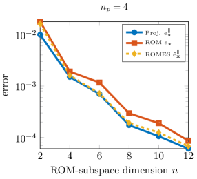
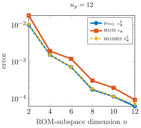
Figure 15: Test case 2. Mean relative ROM error $e_{\mathbf{x}}$ (red), mean relative ROM error after applying the in-plane ROMES correction $\tilde{e}_{\mathbf{x}}^{\mathbin{\|}}$ (yellow), and mean relative projection error $e_{\mathbf{x}}^{\mathbin{\|}}$ (blue) for a varying reduced-subspace dimension $n$ and dual-subspace dimension $n_{p}$. Here, we set $n^{\perp}=0$, $L_{i,j}(\boldsymbol{\theta})=L_{\text{C},i,j}(\boldsymbol{\theta})$, $|\mathcal{D}_{\mathrm{online}}|=600$ and $|\mathcal{D}_{\mathrm{ROMES}}|=400$.

We again perform a similar analysis for the out-of-plane error by comparing the mean relative ROM error $e_{\mathbf{x}}$ with the mean relative ROM error after applying both the in-plane and out-of-plane ROMES corrections $\tilde{e}_{\mathbf{x}}^{\mathbin{\|}+\perp}$ (Eq. (66)) and the mean relative projection error $e_{\mathbf{x}}^{\mathbin{\|}+\perp}$ (Eq. (67)). Figure 16 reports these results for various values of the reduced-subspace dimension $n$, the dual-basis dimension $n_{p}$, and the out-of-plane subspace dimension $n^{\perp}$. We again note that the ROMES correction nearly eliminates both the in- and out-of-plane errors, as $\tilde{e}_{\mathbf{x}}^{\mathbin{\|}+\perp}$ nearly achieves the optimal value of $e_{\mathbf{x}}^{\mathbin{\|}+\perp}$ for all considered parameters.

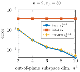
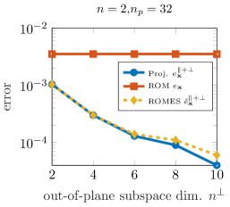
Figure 16: Test case 2. Mean relative ROM error $e_{\mathbf{x}}$ (red), mean relative ROM error after applying the in-plane and out-of-plane ROMES corrections $\tilde{e}_{\mathbf{x}}^{\mathbin{\|}+\perp}$ (yellow), and mean relative projection error $e_{\mathbf{x}}^{\mathbin{\|}+\perp}$ (blue) for a varying reduced-subspace dimension $n$, dual-subspace dimension $n_{p}$, and out-of-plane subspace dimension $n^{\perp}$. Here, we set $L_{i,j}(\boldsymbol{\theta})=L_{\text{C},i,j}(\boldsymbol{\theta})$, $|\mathcal{D}_{\mathrm{ROMES}}|=400$, $|\mathcal{D}_{\mathrm{online}}|=600$

5.2.3 Quantity-of-interest error approximation

As in Section 5.1.3, we now consider the ability of the proposed method to construct statistical models of quantities of interest $\mathbf{\tilde{q}}$ as proposed in Section 4.5. For this purpose, we consider $s={N}$ quantities of interest defined by the von Mises stress at all ${N}$ (unconstrained) grid points in the mesh, i.e.,

$$\begin{split}&\mathbf{q}:\boldsymbol{\nu}\mapsto\mathbf{s}(\mathbf{x}(\boldsymbol{\nu});\boldsymbol{\nu})=\\ &\begin{bmatrix}\sqrt{\frac{(\sigma_{11}(\vec{x}_{1})-\sigma_{22}(\vec{x}_{1}))^{2}+(\sigma_{22}(\vec{x}_{1})-\sigma_{33}(\vec{x}_{1}))^{2}+(\sigma_{33}(\vec{x}_{1})-\sigma_{11}(\vec{x}_{1}))^{2}+6(\sigma_{12}(\vec{x}_{1})^{2}+\sigma_{23}(\vec{x}_{1})^{2}+\sigma_{31}(\vec{x}_{1})^{2})}{2}}\\ \vdots\\ \sqrt{\frac{(\sigma_{11}(\vec{x}_{{N}})-\sigma_{22}(\vec{x}_{{N}}))^{2}+(\sigma_{22}(\vec{x}_{{N}})-\sigma_{33}(\vec{x}_{{N}}))^{2}+(\sigma_{33}(\vec{x}_{{N}})-\sigma_{11}(\vec{x}_{{N}}))^{2}+6(\sigma_{12}(\vec{x}_{{N}})^{2}+\sigma_{23}(\vec{x}_{{N}})^{2}+\sigma_{31}(\vec{x}_{{N}})^{2})}{2}}\end{bmatrix},\end{split}$$

where $\sigma_{ij}=(\mathbf{P}(\mathbf{x})(\mathbf{I}+\nabla\mathbf{x})^{T})_{ij}$, $i,j=1,2,3$ and $\vec{x}_{i}$ denotes the $i$th (unconstrained) grid point in the computational mesh. This is an example of high-dimensional quantity of interest whose error cannot be modeled tractably using the original ROMES method [13], as this would require constructing ${N}$ separate Gaussian-process models. We emphasize that these quantities of interest were not specified during the offline stage (see Remark 4.2).

We set the loss function to $L_{i,j}(\boldsymbol{\theta})=L_{\text{C},i,j}(\boldsymbol{\theta})$, the number of training-parameter instances to $|\mathcal{D}_{\mathrm{ROMES}}|=400$, the dual-basis dimension to $n_{p}=32$. Figure 17 plots the maximum value of the FOM-computed quantity of interest $\max_{i}({q}_{i}(\boldsymbol{\mu}))$ versus both the the maximum value of the ROM-computed quantity of interest $\max_{i}(q_{\mathrm{ROM},i}(\boldsymbol{\mu}))$ and the maximum value of the expected value of the ROMES-corrected quantity of interest $\max_{i}(\mathbb{E}[{\tilde{q}}_{i}(\boldsymbol{\mu})])$ for several values of the reduced-subspace dimension $n$ and out-of-plane subspace dimension $n^{\perp}$ and for $\boldsymbol{\mu}\in\mathcal{D}_{\mathrm{online}}$. Figure 18 reports the associated FVU values, with the FVU defined as

(71) $$\text{FVU}_{\mathbf{q},\max}(\boldsymbol{q})\vcentcolon=\frac{\sum_{\boldsymbol{\mu}\in\mathcal{D}_{\mathrm{online}}}(\max_{i}({q}_{i}(\boldsymbol{\mu}))-\max_{i}(q_{i}(\boldsymbol{\mu})))^{2}}{\sum_{\boldsymbol{\mu}\in\mathcal{D}_{\mathrm{online}}}(\max_{i}({q}_{i}(\boldsymbol{\mu}))-{\bar{q}_{\max}})^{2}},$$

where ${\bar{q}_{\max}}$ denotes the mean value of the quantity of interest $\max_{i}({q}_{i}(\boldsymbol{\mu}))$ for $\boldsymbol{\mu}\in\mathcal{D}_{\mathrm{online}}$. These results show the ability of the proposed method to significantly reduce the quantity-of-interest error without the need for prescribing the quantities of interest in the offline stage (see Remark 4.2). These results also show that performance is improved as the dual-basis dimension $n_{p}$ increases, albeit at increased computational cost.

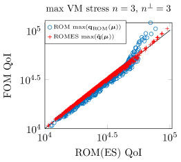
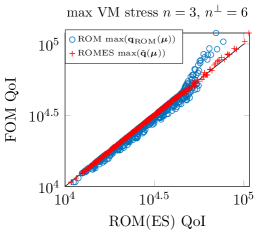
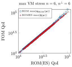
Figure 17: Test case 2. Scatter plot of the the maximum value of the FOM-computed quantity of interest $\max_{i}({q}_{i}(\boldsymbol{\mu}))$ versus both the the maximum value of the ROM-computed quantity of interest $\max_{i}(q_{\mathrm{ROM},i}(\boldsymbol{\mu}))$ (blue circles) and the maximum value of the expected value of the ROMES-corrected quantity of interest $\max_{i}(\mathbb{E}[{\tilde{q}}_{i}(\boldsymbol{\mu})])$ (red crosses) for several values of the reduced-subspace dimension $n$ and for $\boldsymbol{\mu}\in\mathcal{D}_{\mathrm{online}}$. We have employed $n_{p}=32$, and have selected hyperparameters according to Eq. (41) with the specified loss function $L_{i,j}(\boldsymbol{\theta})$. The number of training-parameter instances is $|\mathcal{D}_{\mathrm{ROMES}}|=400$, while $|\mathcal{D}_{\mathrm{ROMES}}|=600$.

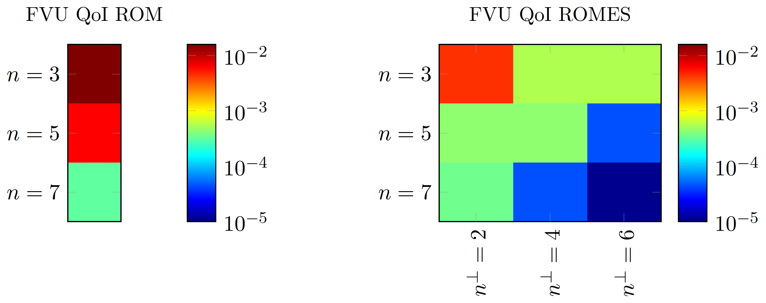
Figure 18: Test case 2. FVU values associated with the ROM-computed quantity of interest $\max_{i}(q_{\mathrm{ROM},i}(\boldsymbol{\mu}))$ and the expected value of the ROMES-corrected quantity of interest $\max_{i}(\mathbb{E}[{\tilde{q}}_{i}(\boldsymbol{\mu})])$ for several values of the reduced-subspace dimension $n$ and $n^{\perp}$. Here, we set $L_{i,j}(\boldsymbol{\theta})=L_{\text{C},i,j}(\boldsymbol{\theta})$, $|\mathcal{D}_{\mathrm{ROMES}}|=1000$ and $n_{p}=32$.

Finally, Figure 19 reports the values of the the mean relative ROM error $e_{q_{i}}$

(72) $$e_{q_{i}}\vcentcolon=\frac{1}{|\mathcal{D}_{\mathrm{online}}|}\sum_{\boldsymbol{\mu}\in\mathcal{D}_{\mathrm{online}}}\left(\frac{|\delta_{q_{i}}(\boldsymbol{\mu})|}{|{q}_{i}(\boldsymbol{\mu})|}\right),$$

and the mean relative ROM error with in- and out-of-plane ROMES correction $\tilde{e}_{{q}_{i}}^{\mathbin{\|}+\perp}$

(73) $$\tilde{e}_{{q}_{i}}^{\mathbin{\|}+\perp}\vcentcolon=\frac{1}{|\mathcal{D}_{\mathrm{online}}|}\sum_{\boldsymbol{\mu}\in\mathcal{D}_{\mathrm{online}}}\left(\frac{|q_{i}(\boldsymbol{\mu})-{s}_{i}(\mathbf{x}_{\text{ROM}}(\boldsymbol{\mu})+\mathbf{\Phi}\mathbb{E}[\tilde{\boldsymbol{\delta}}^{\mathbin{\|}}(\boldsymbol{\mu})]+\mathbf{\Phi}^{\perp}\mathbb{E}[\tilde{\boldsymbol{\delta}}^{\perp}(\boldsymbol{\mu})];\boldsymbol{\mu})|}{|q_{i}(\boldsymbol{\mu})|}\right),$$

for $i=1,\ldots,{N}$ as distributed over the physical domain. We observe that applying both the in-plane and out-of-plane ROMES correction yields a very small mean relative error, thereby illustrating the ability of the method to accurately model the error in field quantities.

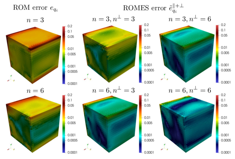
Figure 19: Test case 2. The values of the mean relative ROM error $e_{q_{i}}$ (left column) and the mean relative ROM error with in- and out-of-plane ROMES correction $\tilde{e}_{{q}_{i}}^{\mathbin{\|}+\perp}$ for $i=1,\ldots,{N}$ (center and right columnes) as distributed over the physical domain. Here, we set $L_{i,j}(\boldsymbol{\theta})=L_{\text{C},i,j}(\boldsymbol{\theta})$, $|\mathcal{D}_{\mathrm{ROMES}}|=400$, $|\mathcal{D}_{\mathrm{online}}|=600$ and $n_{p}=12$.

5.2.4 Computational efficiency

As in Section 5.1.4, we now analyze the computational efficiency of the proposed method with respect to a ‘ROM-only’ approach. As discussed in Remark 4.3, we expect the proposed method to yield favorable performance relative to the linear problem considered in Section 5.1, as the dual ROM equations (25) are always linear in their first argument, even when the ROM equations (4) are nonlinear in their first argument; thus, relative to the (primal) ROM solve, the dual solves are computationally inexpensive.

We repeat the study executed in Section 5.1.4, and subject the ‘ROM-only’ method, the proposed method with a ROMES in-plane correction only, and the proposed method with both an in-plane and out-of-plane correction to a wide range of parameter values. In particular, we consider all combinations of $n\in\{2,\ldots,10\}$, $n_{p}\in\{12,22,32\}$ (not relevant to the ‘ROM-only’ method), and $n^{\perp}\in\{2,\ldots,10\}$ (not relevant to the ‘ROM-only’ method or the proposed method with in-plane correction only). Figure 20 reports these results and associated Pareto fronts.

These results show that the proposed method with both in-plane and out-of-plane ROMES corrections are Pareto dominant. Specifically, for a fixed wall time, the method yields approximately one order of magnitude in error reduction; for a fixed error, the method yields approximately a 30% reduction in wall time. Furthermore, this approach provides a statistical model of the FOM state and quantities of interest, which is not provided by the ‘ROM-only’ approach. Thus, the proposed method has demonstrated superior performance not only in its computational efficiency, but also in its ability to quantify the ROM-induced epistemic uncertainty, which is essential for rigorous integration into uncertainty-quantification applications. We note that the proposed method with an in-plane ROMES correction only yields similar performance to the ‘ROM-only’ approach. This occurs because the ROM in-plane errors are already quite small; this was previously discussed in Section 5.2.2 and observed in Figure 15.

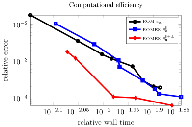
Figure 20: Test case 2. Computational efficiency of the ‘ROM-only’ approach (ROM $e_{\mathbf{x}}$), the proposed method with a ROMES in-plane correction only (ROMES $\tilde{e}_{\mathbf{x}}^{\mathbin{\|}}$), and the proposed method with both an in-plane and out-of-plane correction (ROMES $\tilde{e}_{\mathbf{x}}^{\mathbin{\|}+\perp}$) three approaches over a range of method parameters, and associated Pareto fronts. Here, the relative error corresponds to $\tilde{e}_{\mathbf{x}}^{\mathbin{\|}+\perp}$ (Eq. (66)), and the wall time for the simulations relative to that incurred by the full-order model. Note that the proposed method with both in-plane and out-of-plane ROMES correction is Pareto dominant.

6 Conclusions

This work has proposed a technique for constructing a statistical closure model for reduced-order models (ROMs) applied to stationary systems. The proposed method applies the ROMES method to construct a statistical model for the state error through constructing statistical models for the generalized coordinates characterizing both the in-plane error (i.e., the closure model) and a low-dimensional approximation of the out-of-plane error. Key ingredients of the method include (1) cheaply computable error indicators associated with a ROM-approximated dual-weighted residual (Section 4.2), (2) a Gaussian-process model to map these error indicators to a random variable for the error generalized coordinates (Section 4.3, (3) a cross-validation procedure for targeting specific statistical-validation criteria (Section 4.4), and (4) a way to statistically quantify the error in any quantity of interest a posteriori by propagating the state-error model through the associated functional.

Numerical experiments demonstrated the ability of the method to accurately model both the in-plane and out-of-plane errors (Figures 5, 6, 15, 16), quantity-of-interest errors (Figures 7, 8, 9, 17, 18, 19), and realize a more computationally efficient methodolgy than a ‘ROM-only approach in the case of nonlinear stationary systems (Figure 20).

In both numerical experiments, it was not possible to rigorously validate the Gaussian assumption underlying the proposed statistical model (Figures 4 and 14). As such, we proposed the use of specific loss functions (e.g., matching $\omega$-prediction intervals, minimizing the Komolgorov–Smirnov statistic) for hyperparameter selection that enabled the statistical model to satisfy a subset of targeted statistical-validation criteria (Tables 2 and 4).

Future work includes developing stochastic-process models associated with different distributions; this will enable a wider range of statistical-validation criteria to be met by the constructed model. In addition, we aim to extend the proposed methodology to dynamical systems.

References

- [1] D. Amsallem, M. Zahr, Y. Choi, and C. Farhat, Design optimization using hyper-reduced-order models, Structural and Multidisciplinary Optimization, 51 (2015), pp. 919–940.
- [2] H. Antil, M. Heinkenschloss, and D. C. Sorensen, Application of the discrete empirical interpolation method to reduced order modeling of nonlinear and parametric systems, in Reduced Order Methods for Modeling and Computational Reduction, A. Quarteroni and G. Rozza, eds., vol. 9 of Modeling, Simulation and Applications, (MS&A) series, Springer, Switzerland, 2014, pp. 101–136.
- [3] P. Astrid, S. Weiland, K. Willcox, and T. Backx, Missing point estimation in models described by proper orthogonal decomposition, IEEE Trans. Automat. Control, 53 (2008), pp. 2237–2251.
- [4] M. Barrault, Y. Maday, N. Nguyen, and A. Patera, An empirical interpolation method: application to efficient reduced-basis discretization of partial differential equations, C. R. Math., 339 (2004), pp. 667–672.
- [5] P. Benner, S. Gugercin, and K. Willcox, A survey of projection-based model reduction methods for parametric dynamical systems, SIAM Review, 57 (2015), pp. 483–531.
- [6] T. Bui-Thanh, K. Willcox, and O. Ghattas, Model reduction for large-scale systems with high-dimensional parametric input space, SIAM Journal on Scientific Computing, 30 (2008), pp. 3270–3288.
- [7] T. Bui-Thanh, K. Willcox, and O. Ghattas, Parametric reduced-order models for probabilistic analysis of unsteady aerodynamic applications, AIAA Journal, 46 (2008), pp. 2520–2529.
- [8] K. Carlberg, Adaptive -refinement for reduced-order models, International Journal for Numerical Methods in Engineering, 102 (2015), pp. 1192–1210.
- [9] K. Carlberg, M. Barone, and H. Antil, Galerkin v. least-squares Petrov–Galerkin projection in nonlinear model reduction, Journal of Computational Physics, 330 (2017), pp. 693–734.
- [10] K. Carlberg, C. Farhat, and C. Bou-Mosleh, Efficient non-linear model reduction via a least-squares Petrov–Galerkin projection and compressive tensor approximations, International Journal for Numerical Methods in Engineering, 86 (2011), pp. 155–181.
- [11] K. Carlberg, C. Farhat, J. Cortial, and D. Amsallem, The GNAT method for nonlinear model reduction: effective implementation and application to computational fluid dynamics and turbulent flows, Journal of Computational Physics, 242 (2013), pp. 623–647.
- [12] S. Chaturantabut and D. Sorensen, Nonlinear Model Reduction via Discrete Empirical Interpolation, SIAM Journal on Scientific Computing, 32 (2010), pp. 2737–2764.
- [13] M. Drohmann and K. Carlberg, The ROMES method for statistical modeling of reduced-order-model error, SIAM/ASA Journal on Uncertainty Quantification, 3 (2015), pp. 116–145.
- [14] M. S. Eldred, A. A. Giunta, S. S. Collis, N. A. Alexandrov, and R. M. Lewis, Second-order corrections for surrogate-based optimization with model hierarchies, in 10th AIAA/ISSMO Multidisciplinary Analysis and Optimization Conference, Albany, NY, no. AIAA Paper 4457, 2004.
- [15] B. A. Freno and K. T. Carlberg, Machine-learning error models for approximate solutions to parameterized systems of nonlinear equations, arXiv e-print, 1808.02097 (2018).
- [16] S. E. Gano, J. E. Renaud, and B. Sanders, Hybrid variable fidelity optimization by using a kriging-based scaling function, AIAA Journal, 43 (2005), pp. 2422–2433.
- [17] M. Grepl, Y. Maday, N. Nguyen, and A. Patera, Efficient reduced-basis treatment of nonaffine and nonlinear partial differential equations, ESAIM Math. Model. Numer. Anal., 41 (2007), pp. 575–605.
- [18] S. Hain, M. Ohlberger, M. Radic, and K. Urban, A hierarchical a posteriori error estimator for the reduced basis method, arXiv e-print, 1802.03298 (2018).
- [19] J. S. Hesthaven, G. Rozza, B. Stamm, et al., Certified reduced basis methods for parametrized partial differential equations, Springer, 2016.
- [20] M. Hinze and M. Kunkel, Residual based sampling in pod model order reduction of drift-diffusion equations in parametrized electrical networks, ZAMM-Journal of Applied Mathematics and Mechanics/Zeitschrift für Angewandte Mathematik und Mechanik, 92 (2012), pp. 91–104.
- [21] P. Holmes, J. Lumley, and G. Berkooz, Turbulence, Coherent Structures, Dynamical Systems and Symmetry, Cambridge University Press, 1996.
- [22] D. Huynh, D. Knezevic, Y. Chen, J. S. Hesthaven, and A. Patera, A natural-norm successive constraint method for inf-sup lower bounds, Computer Methods in Applied Mechanics and Engineering, 199 (2010), pp. 1963–1975.
- [23] D. B. P. Huynh, G. Rozza, S. Sen, and A. T. Patera, A successive constraint linear optimization method for lower bounds of parametric coercivity and inf–sup stability constants, Comptes Rendus Mathematique, 345 (2007), pp. 473–478.
- [24] T. Iliescu and Z. Wang, Variational multiscale proper orthogonal decomposition: Convection-dominated convection-diffusion-reaction equations, Mathematics of Computation, 82 (2013), pp. 1357–1378.
- [25] T. Lassila, A. Manzoni, and G. Rozza, On the approximation of stability factors for general parametrized partial differential equations with a two-level affine decomposition, ESAIM Math. Modelling Numer. Anal., 46 (2012), pp. 1555–1576.
- [26] P. A. LeGresley, Application of Proper Orthogonal Decomposition (POD) to Design Decomposition Methods, PhD thesis, Stanford University, 2006.
- [27] Y. Maday, N. C. Nguyen, A. T. Patera, and G. S. H. Pau, A general multipurpose interpolation procedure: the magic points, Commun. Pure Appl. Anal., 8 (2009), pp. 383–404.
- [28] A. Manzoni and F. Negri, Heuristic strategies for the approximation of stability factors in quadratically nonlinear parametrized PDEs, Adv. Comput. Math., 41 (2015), pp. 1255–1288.
- [29] A. Manzoni, S. Pagani, and T. Lassila, Accurate solution of Bayesian inverse uncertainty quantification problems combining reduced basis methods and reduction error models, SIAM/ASA Journal on Uncertainty Quantification, 4 (2016), pp. 380–412.
- [30] A. March and K. Willcox, Provably convergent multifidelity optimization algorithm not requiring high-fidelity derivatives, AIAA Journal, 50 (2012), pp. 1079–1089.
- [31] M. Meyer and H. Matthies, Efficient model reduction in non-linear dynamics using the Karhunen-Loève expansion and dual-weighted-residual methods, Computational Mechanics, 31 (2003), pp. 179–191.
- [32] F. Negri, A. Manzoni, and D. Amsallem, Efficient model reduction of parametrized systems by matrix discrete empirical interpolation, J. Comput. Phys., 303 (2015), pp. 431–454.
- [33] L. W.-T. Ng and M. Eldred, Multifidelity uncertainty quantification using non-intrusive polynomial chaos and stochastic collocation, in Structures, Structural Dynamics, and Materials and Co-located Conferences, American Institute of Aeronautics and Astronautics, Apr. 2012, pp. –.
- [34] S. Pagani, Reduced-order models for inverse problems and uncertainty quantification in cardiac electrophysiology, PhD thesis, Politecnico di Milano, 2017.
- [35] S. Pagani, A. Manzoni, and A. Quarteroni, Efficient state/parameter estimation in nonlinear unsteady PDEs by a reduced basis ensemble Kalman filter, SIAM/ASA Journal on Uncertainty Quantification, 5 (2017), pp. 890–921.
- [36] S. Pan and K. Duraisamy, Data-driven discovery of closure models, arXiv e-print, 1803.09318 (2018).
- [37] A. Quarteroni, A. Manzoni, and F. Negri, Reduced Basis Methods for Partial Differential Equations. An Introduction, vol. 92 of Unitext Series, Springer International Publishing, 2016.
- [38] C. Rasmussen and C. Williams, Gaussian Processes for Machine Learning, MIT Press, 2006.
- [39] T. Rebollo, A. Enrique, M. Mármol, F. Ballarin, and G. Rozza, On a certified smagorinsky reduced basis turbulence model, SIAM Journal on Numerical Analysis, 55 (2017), pp. 3047–3067.
- [40] G. Rozza, D. B. P. Huynh, and A. T. Patera, Reduced basis approximation and a posteriori error estimation for affinely parametrized elliptic coercive partial differential equations, Archives of Computational Methods in Engineering, 15 (2007), p. 1.
- [41] S. Trehan, K. Carlberg, and L. Durlofsky, Error modeling for surrogates of dynamical systems using machine learning, International Journal for Numerical Methods in Engineering, 112 (2017), pp. 1801–1827.
- [42] K. Veroy and A. Patera, Certified real-time solution of the parametrized steady incompressible navier–stokes equations: rigorous reduced-basis a posteriori error bounds, International Journal for Numerical Methods in Fluids, 47 (2005), pp. 773–788.
- [43] Z. Wang, I. Akhtar, J. Borggaard, and T. Iliescu, Proper orthogonal decomposition closure models for turbulent flows: a numerical comparison, Computer Methods in Applied Mechanics and Engineering, 237 (2012), pp. 10–26.
- [44] K. Willcox, Unsteady flow sensing and estimation via the gappy proper orthogonal decomposition, Computers & fluids, 35 (2006), pp. 208–226.
- [45] D. Wirtz, D. C. Sorensen, and B. Haasdonk, A-posteriori error estimation for DEIM reduced nonlinear dynamical systems, SIAM J. Sci. Comput, 36 (2014), pp. A311–338.
- [46] Y. Wu and U. Hetmaniuk, Adaptive training of local reduced bases for unsteady incompressible Navier–Stokes flows, International Journal for Numerical Methods in Engineering, 103 (2015), pp. 183–204.
- [47] X. Xie, M. Mohebujjaman, L. Rebholz, and T. Iliescu, Data-driven filtered reduced order modeling of fluid flows, SIAM Journal on Scientific Computing, 40 (2018), pp. B834–B857.
- [48] M. Yano and A. T. Patera, An LP empirical quadrature procedure for reduced basis treatment of parametrized nonlinear PDEs, Computer Methods in Applied Mechanics and Engineering, (2018).
- [49] M. Zahr, K. Carlberg, and D. Kouri, An efficient, globally convergent method for optimization under uncertainty using adaptive model reduction and sparse grids, arXiv e-print, 1811.00177 (2018).
- [50] M. J. Zahr and C. Farhat, Progressive construction of a parametric reduced-order model for PDE-constrained optimization, International Journal for Numerical Methods in Engineering, 102 (2015), pp. 1111–1135.