Causal mediation analysis for stochastic interventions

Abstract

Mediation analysis in causal inference has traditionally focused on binary exposures and deterministic interventions, and a decomposition of the average treatment effect in terms of direct and indirect effects. In this paper we present an analogous decomposition of the population intervention effect, defined through stochastic interventions on the exposure. Population intervention effects provide a generalized framework in which a variety of interesting causal contrasts can be defined, including effects for continuous and categorical exposures. We show that identification of direct and indirect effects for the population intervention effect requires weaker assumptions than its average treatment effect counterpart, under the assumption of no mediator-outcome confounders affected by exposure. In particular, identification of direct effects is guaranteed in experiments that randomize the exposure and the mediator. We discuss various estimators of the direct and indirect effects, including substitution, re-weighted, and efficient estimators based on flexible regression techniques, allowing for multivariate mediators. Our efficient estimator is asymptotically linear under a condition requiring $n^{1/4}$-consistency of certain regression functions. We perform a simulation study in which we assess the finite-sample properties of our proposed estimators. We present the results of an illustrative study where we assess the effect of participation in a sports team on BMI among children, using mediators such as exercise habits, daily consumption of snacks, and overweight status.

1 Introduction

Mediation analysis is a powerful analytical tool that allows scientists to unveil the mechanisms through which causal effects operate. The development of tools for mediation analysis has a long history in the statistical sciences, starting with the early work of Wright (1921, 1934) on path analysis, which provided the foundations for the later development of mediation analysis using structural equation models (Goldberger, 1972). Indeed, one of the most widely used mediation analysis methods is based on structural equations (Baron and Kenny, 1986). Recent decades have seen a revolution in the field of causal inference from observational and randomized studies, starting with the seminal work of Rubin (1974) on the potential outcomes framework, which is itself rooted in ideas dating back to Neyman (1923). More recently, Pearl (1995, 2000) has developed a causal inference framework using non-parametric structural equation models, directed acyclic graphs, and the so-called do-calculus. Related approaches have been proposed by Robins (1986), Spirtes et al. (2000), Dawid (2000), and Richardson and Robins (2013). These frameworks allow researchers to define causal effects non-parametrically, and to assess the conditions under which causal effects can be identified from data. In particular, novel tools have uncovered important limitations of the earlier work on parametric structural equation models for mediation analysis (Pearl, 1998; Imai et al., 2010). Essentially, structural equation models impose implausible assumptions on the data generating mechanism, and are thus of limited applicability to complex phenomena in biology, health, economics, and the social sciences. For example, modern causal models have revealed the incorrectness of the widely popular method of Baron and Kenny (1986) in several important cases, such as in the presence of confounders of the mediator-outcome relationship (Cole and Hernán, 2002).

Using the potential outcomes framework, Robins and Greenland (1992) introduced a non-parametric decomposition of the causal effect of a binary exposure into so-called natural indirect and direct effects. The indirect effect quantifies the effect on the outcome through the mediator and the direct effect quantifies the effect through all other mechanisms. Pearl (2001) arrived at an equivalent effect decomposition using non-parametric structural equation models. The identification of these natural (in)direct effects relies on so-called cross-world counterfactual independencies, i.e., independencies on counterfactual variables indexed by distinct hypothetical interventions. An important consequence of this definition is that the natural (in)direct effect is not identifiable in a randomized trial, which is problematic as it implies that scientific claims obtained from these models are not falsifiable through experimentation (Popper, 1934; Dawid, 2000; Robins and Richardson, 2010).

In an attempt to solve these problems, several authors have proposed methods that do away with cross-world counterfactual independencies. These methods can be divided in two types: identification of bounds (Robins and Richardson, 2010; Tchetgen and Phiri, 2014; Miles et al., 2015), and alternative definitions of the (in)direct effect (Petersen et al., 2006; van der Laan and Petersen, 2008; Vansteelandt and VanderWeele, 2012; VanderWeele et al., 2014). Here, we take the second approach, defining the (in)direct effect in terms of a decomposition of the total effect of a stochastic intervention on the population exposure.

Most causal inference problems consider deterministic interventions that set each unit’s exposure to some fixed value that could be a function of the unit’s baseline variables. Stochastic interventions are a generalization of this framework, and are loosely defined as interventions which yield an exposure that is a random variable after conditioning on baseline variables. Estimation of total effects of stochastic interventions was first considered by Stock (1989) and has been the subject of recent study (Robins et al., 2004; Didelez et al., 2006; Tian, 2008; Pearl, 2009; Taubman et al., 2009; Stitelman et al., 2010; Díaz and van der Laan, 2013; Dudík et al., 2014; Haneuse and Rotnitzky, 2013; Young et al., 2014). Particularly relevant to this work are the methods of Díaz and van der Laan (2012); Haneuse and Rotnitzky (2013) who define total effects for modified treatment policies, and Kennedy (2018a), who study identification and estimation of the total the effect of propensity score interventions that shift a binary exposure distribution. These papers do not address decomposition of the effects of stochastic interventions on the exposure into direct and indirect effects, which is the central theme of our manuscript.

Our methods are also related to a family of new direct and indirect effects (Didelez et al., 2006; VanderWeele et al., 2014; Lok, 2016; Vansteelandt and Daniel, 2017; Zheng and van der Laan, 2017; Rudolph et al., 2017; Lok, 2019), which have been collectively termed interventional effects (Nguyen et al., 2019). This family of effects deals with binary exposures and deterministic interventions on the exposure, and is thus not entirely related to our approach, which deals with both continuous and categorical exposures and stochastic interventions on the exposure. Like the effects on the treated of Vansteelandt and VanderWeele (2012), interventional effects share the no-cross-world-independence property of our methods. The interested reader is referred to Nguyen et al. (2019) for a taxonomy of the several mediation analyses proposed in the causal inference literature up to date.

Stochastic interventions have analytical advantages compared to their deterministic counterparts, such as allowing the seamless definition of causal effects for continuous exposures with an interpretation that is familiar to regular users of linear regression adjustment. For example, Haneuse and Rotnitzky (2013) assess the effect of an intervention that reduces a patient’s operating time (i.e., the time spent in surgery) on the risk of post-operative outcomes among patients undergoing surgical resection non-small-cell lung cancer. Díaz and van der Laan (2012) study the effect of increasing the amount of leisure time physical activity in the elderly on subsequent all-cause mortality. Díaz and van der Laan (2013) study the effect of a (hypothetical) policy that enforces pollution levels below a certain cutoff point. Kennedy (2018a) shows that stochastic interventions can also be used in longitudinal studies to define and estimate total effects without relying on the positivity assumption.

In this article, we propose a decomposition of the effect of a stochastic intervention into a direct and an indirect effect, with interpretation analogous to that originally proposed by Robins and Greenland (1992) and Pearl (2001). We show that the identification of (in)direct effects based on stochastic interventions does not require cross-world counterfactual independencies, therefore yielding scientific results that can be tested through experimentation on both the exposure and mediator. Of high practical relevance, our proposal also allows the definition and estimation of non-parametric mediated effects for continuous exposures, a problem for which no methods or software exist. Parametric mediation methods such as those discussed by Vansteelandt et al. (2012) induce unquantifiable amounts of bias by imposing untestable and implausible parametric assumptions on the distribution of cross-world counterfactuals.

We develop a one-step non-parametric estimator based on the efficient influence function, incorporating flexible regression tools from the machine learning literature, and provide $n^{1/2}$-rate convergence and asymptotic linearity results. We propose methods to use these asymptotic distributions to construct confidence regions and to test the null hypothesis of no direct effect. Our estimator has roots in semiparametric estimation theory (e.g., Pfanzagl and Wefelmeyer, 1985; Begun et al., 1983; van der Vaart, 1991; Newey, 1994; Bickel et al., 1997), and in the targeted learning framework of van der Laan and Rubin (2006); van der Laan and Rose (2011, 2018). In particular, we use cross-fitting in order to obtain $n^{1/2}$-convergence of our estimators while avoiding entropy conditions that may be violated by the data adaptive estimators we use (Zheng and van der Laan, 2011; Chernozhukov et al., 2018). Our estimators use a re-parameterization of certain integrals as conditional expectations in order to accommodate multivariate mediators. Software implementing our methods is provided in the form of an open source R package freely available on GitHub.

2 Mediation analysis for population intervention effects

Let $A$ denote a continuous or categorical exposure variable, let $Y$ denote a continuous or binary outcome, let $Z$ denote a multivariate mediator, and let $W$ denote a vector of observed covariates. Let $O=(W,A,Z,Y)$ represent a random variable with distribution $\mathbb{P}$. We use $\mathbb{P}_{n}$ to denote the empirical distribution of a sample of $n$ i.i.d. observations $O_{1},\ldots,O_{n}$. We let $\mathbb{P}f=\int f(o)\mathrm{d}\mathbb{P}(o)$ for a given function $f(o)$, and use $\mathbb{E}$ to denote expectations with respect to $\mathbb{P}$. We assume $\mathbb{P}\in\mathcal{M}$, where $\mathcal{M}$ is the nonparametric statistical model defined as all continuous densities on $O$ with respect to a dominating measure $\nu$. Let $p$ denote the corresponding probability density function. We use $g(a\mid w)$ to denote the probability density function or the probability mass function of $A$ conditional on $W=w$; $m(a,z,w)$ and $b(a,w)$ to denote the outcome regression functions $\mathbb{E}(Y\mid A=a,Z=z,W=w)$ and $\mathbb{E}(Y\mid A=a,W=w)$, respectively; and $e(a\mid z,w)$ to denote the conditional density or probability mass function of $A$ conditional on $(Z,W)$. Let $g(a\mid w)$ be dominated by a measure $\kappa(a)$ (e.g., the counting measure for binary $A$ and the Lebesgue measure for continuous $A$). We use $q(z\mid a,w)$ and $r(z\mid w)$ to denote the corresponding conditional densities of $Z$. The parametrization $e=gq/r$ will prove fundamental in the construction of our estimators, since it will allow us to avoid estimation of multivariate conditional densities. A similar parameterization is used by Zheng and van der Laan (2012) to estimate mediated effects under deterministic interventions. We use $\cal W,\cal A,\cal Z$ and $\cal Y$ to denote the support of the corresponding random variables.

We formalize the definition of our counterfactual variables using the following non-parametric structural equation model (NPSEM), but note that equivalent methods may be developed by taking the counterfactual variables as primitives. Assume

$$W=f_{W}(U_{W});\ A=f_{A}(W,U_{A});\ Z=f_{Z}(W,A,U_{M});\ Y=f_{Y}(W,A,ZU_{Y}).$$ (1)

This set of equations represents a mechanistic model assumed to generate the observed data $O$; furthermore, it encodes several fundamental assumptions. First, an implicit temporal ordering is assumed — that is, $Y$ occurs after $Z$, $A$ and $W$; $Z$ occurs after $A$ and $W$; and $A$ occurs after $W$. Second, each variable (i.e., $\{W,A,Z,Y\}$) is assumed to be generated from the corresponding deterministic function (i.e., $\{f_{W},f_{A},f_{Z},f_{Y}\}$) of the observed variables that precede it temporally, plus an exogenous variable, denoted by $U$. Each exogenous variable is assumed to contain all unobserved causes of the corresponding observed variable. Independence assumptions on $U=(U_{W},U_{A},U_{Z},U_{Y})$ necessary for identification will be clarified in Section 2.1. Furthermore, we note that we have explicitly excluded outcome-mediator confounders which are affected by exposure. Mediation analysis in the presence of a such variables is notoriously hard (Avin et al., 2005); the adaptation of our methods to this problem is possible but it requires a new set of tools which is out of the scope of this paper.

Causal effects are defined in terms of hypothetical interventions on the NPSEM (1). In particular, consider an intervention in which the equation corresponding to $A$ is removed, and the exposure is drawn from a user-specified distribution $g_{\delta}(a\mid w)$, which may depend on $g$ and is indexed by a user-specified parameter $\delta$. We assume without loss of generality that $g_{\delta=0}=g$. Let $A_{\delta}$ denote a draw from $g_{\delta}(a\mid w)$. Alternatively, such modifications can sometimes be described in terms of an intervention in which the equation corresponding to $A$ is removed and the exposure is set equal to a hypothetical regime $d(A,W)$. Regime $d$ depends on the natural (that is, under no intervention) exposure level $A$ and covariates $W$. The latter intervention is sometimes referred to as depending on the natural value of exposure, or as a modified treatment policy (Haneuse and Rotnitzky, 2013). Young et al. (2014) provide a discussion of the differences and similarities in the interpretation and identification of these two interventions. Below, we discuss two examples of stochastic interventions: modified treatment policies, and exponential tilting.

Example 1 (Modified treatment policy (Haneuse and Rotnitzky, 2013)).

Let $A$ denote a continuous exposure, such as operating time in non-small-cell lung cancer. Assume the distribution of $A$ conditional on $W=w$ is supported in the interval $(l(w),u(w))$. That is, the minimum possible operating time for an individual with covariates $W=w$ is $l(w)$. Then one may define a hypothetical post-intervention exposure $A_{\delta}=d(A,W)$, where

$$d(a,w)=\begin{cases}a-\delta&\text{if }a>l(w)+\delta\\ a&\text{if }a\leq l(w)+\delta,\end{cases}$$ (2)

where $0<\delta<u(w)$ is an arbitrary user-given value. Interesting modifications to this regime may be obtained by allowing $\delta$ to be a function of $w$, therefore allowing the researcher to specify a different change in operating time as a function of covariates such as comorbidities, age, etc. This intervention was first introduced by Díaz and van der Laan (2012), and has been further discussed in Díaz and van der Laan (2018) and Haneuse and Rotnitzky (2013).

Example 2 (Exponential tilting).

We can alternatively define a tilted intervention distribution as

$$g_{\delta}(a\mid w)=\frac{\exp(\delta a)g(a\mid w)}{\int\exp(\delta a)g(a\mid w)\mathrm{d}\kappa(a)},$$ (3)

for $\delta\in\mathbb{R}$, and let the hypothetical post-intervention exposure $A_{\delta}$ be a random draw from $g_{\delta}$, conditional on the natural value of the observed covariates $W$. For binary $A$, Kennedy (2018a) proposed evaluating the total effect of a binary exposure $A$ in terms of incremental propensity score interventions that replace the propensity score $g(1\mid w)$ with a shifted version based on multiplying the odds of exposure by a user-given parameter $\delta^{\prime}$. In particular, the post-intervention propensity score is given by

$$g_{\delta^{\prime}}(1\mid w)=\frac{\delta^{\prime}g(1\mid w)}{\delta^{\prime}g(1\mid w)+1-g(1\mid w)},$$ (4)

for $0<\delta^{\prime}<\infty$. The proposal of Kennedy (2018a) is thus a case of exponential tilting (3) under the parameterization $\delta^{\prime}=\exp(\delta)$. This choice of parameterization is motivated by the fact that $\delta^{\prime}$ can be interpreted as an odds ratio indicating how the intervention changes the odds of exposure. The extremes of $\delta^{\prime}=0$ and $\delta^{\prime}=\infty$ correspond to the standard interventions $A=0$ and $A=1$ considered in the definition of the average treatment effect.

We now turn our attention to defining the population intervention effect (PIE) of $A$ on $Y$. To proceed, for any values $(a,z)$, consider the counterfactual outcome $Y(a,z)=f_{Y}(W,a,z,U_{Y}).$, and the counterfactual mediator $Z(a)=f_{Z}(W,a,U_{Z})$. The counterfactual $Y(a,z)$ is the outcome in a hypothetical world in which $(A,Z)=(a,z)$ is fixed externally. The PIE is defined as a contrast comparing the expectation of the outcome under no intervention with the expectation of the counterfactual outcome obtained under an intervention $A_{\delta}$:

$$\psi(\delta)=\mathbb{E}\{Y(A_{\delta})-Y\}.$$

Note that the interpretation of the PIE depends on the stochastic intervention considered. For example, for the modified treatment policies of Example 1, the PIE describes the difference in outcomes obtained by a reduction of $\delta$ in operating time. In the case of the incremental propensity score intervention (4), the PIE is interpreted as the difference in outcomes obtained by an intervention under which the odds of exposure is $\delta^{\prime}$ times higher compared to current practice.

Since $A$ is a cause of $Z$, an intervention that changes the exposure to $A_{\delta}$ also induces a counterfactual mediator $Z(A_{\delta})$. As a consequence of the consistency implied by the NPSEM, we have $Y(A,Z)=Y$. Similarly, the law of composition (Pearl, 2000) allows us to write $Y(A_{\delta},Z(A_{\delta}))=Y(A_{\delta})$. Thus, the PIE may be decomposed in terms of a population intervention direct effect (PIDE) and a population intervention indirect effect (PIIE):

$$\psi(\delta)=\overbrace{\mathbb{E}\{Y(A_{\delta},Z(A_{\delta}))-Y(A_{\delta},Z)\}}^{\text{PIIE}}+\overbrace{\mathbb{E}\{Y(A_{\delta},Z)-Y(A,Z)\}}^{\text{PIDE}}.$$ (5)

This decomposition of the PIE as the sum of direct and indirect effects has an interpretation analogous to the corresponding standard decomposition of the average treatment effect (Pearl, 2001). In particular, the direct effect represents the effect of an intervention that changes the distribution of the exposure while keeping the distribution of the mediators fixed at the value that it would have taken under no intervention. The indirect effect measures the effect of an indirect intervention on the mediators generated by intervening on the exposure, while holding the intervention on the exposure constant.

The intervention in Example 1 arises naturally as a modified treatment policy. In contrast, the intervention in Example 2 arises directly as a stochastic intervention that modifies the distribution of the variables — it is unclear as of yet whether this quantity may be interpreted as a modified treatment policy. Drawing on the work of Haneuse and Rotnitzky (2013), we make the following assumption for modified treatment policies, which ensures that we can use the change of variable formula when computing integrals over $\cal A$. This is useful for studying properties of the parameter and estimators we propose.

A1Piecewise smooth invertibility.

For each $w\in\cal W$, assume that the interval ${\cal I}(w)=(l(w,),u(w))$ may be partitioned into subintervals ${\cal I}_{\delta,j}(w):j=1,\ldots,J(w)$ such that $d(a,w)$ is equal to some $d_{j}(a,w)$ in ${\cal I}_{\delta,j}(w)$ and $d_{j}(\cdot,w)$ has inverse function $h_{j}(\cdot,w)$ with derivative $h_{j}^{\prime}(\cdot,w)$.

Under this assumption, the distribution of a modified treatment policy $A_{\delta}=d(A,W)$ may be recovered through (see Haneuse and Rotnitzky, 2013):

$$g_{\delta}(a\mid w)=\sum_{j=1}^{J(w)}I_{\delta,j}\{h_{j}(a,w),w\}g\{h_{j}(a,w)\mid w\}h_{j}^{\prime}(a,w),$$ (6)

where $I_{\delta,j}\{u,w\}=1$ if $u\in{\cal I}_{\delta,j}(w)$ and $I_{\delta,j}\{u,w\}=0$ otherwise. In Example 1, the stochastic intervention becomes

$$g_{\delta}(a\mid w)=g(a\mid w)\mathds{1}\{l(w)\leq a\leq l(w)+\delta\}+g(a+\delta\mid w)\mathds{1}\{l(w)\leq a\leq u(w)-\delta\}.$$

Therefore, under A1, a modified treatment policy may also be represented as a change by which the equation $f_{A}$ is removed from the NPSEM and $A$ is replaced by a draw $A_{\delta}$ from the distribution $g_{\delta}(a\mid w)$. As a result of these two representations, the intervention may be interpreted in two different ways: (i) a change in the probabilistic mechanism used to assign exposure level, and (ii) a subject-specific change in exposure from $A$ to $A_{\delta}=d(A,W)$, where only interpretation (i) requires A1. Note, however, that the population distribution of the exposure is the same under both interventions (Young et al., 2014); thus, both representations lead to exactly the same marginal counterfactual outcome distributions.

Several estimators of the functional $\psi(\delta)$ have previously been proposed. For the case of a continuous exposure, Díaz and van der Laan (2012) developed inverse probability weighted, outcome regression, and doubly robust estimators based on the framework of targeted minimum loss-based estimation (TMLE) (van der Laan and Rose, 2011), using data adaptive estimators of the relevant nuisance parameters. Díaz and van der Laan (2018) improved on the previous methodology by constructing a TMLE algorithm with lower computational complexity that preserves the desirable asymptotic properties of the original approach. Haneuse and Rotnitzky (2013) propose estimators that rely on correctly specified parametric models. Such methods are of limited applicability since they are reliable only in situations where the nuisance parameters involve only few categorical variables, where correctly specified (that is, saturated) parametric models can conscientiously be constructed. For the binary case with $g_{\delta}$ as in Example 2, Kennedy (2018a) proposed an estimator for $\psi(\delta)$. This estimator is efficient, asymptotically linear, and it allows incorporation of data adaptive estimators of the nuisance parameters.

Since $\mathbb{E}(Y)$ is trivially estimated by the empirical mean in the sample, our optimality theory and estimators focus on $\theta(\delta)=\mathbb{E}\{Y(A_{\delta},Z)\}$. We present two types of results: for general modified treatment policies satisfying (A1), and for the particular stochastic intervention of Example 2. We compare the assumptions required for both.

2.1 Identification

In this section we introduce the counterfactual variable $Y(a,z)$, defined as the outcome that would be observed in a hypothetical world in which $\mathbb{P}\{(A,Z)=(a,z)\}=1$. This is the same counterfactual variable that is often used to perform mediation analyses on the average treatment effect (Robins and Greenland, 1992; Pearl, 2001).

We introduce the following identification assumptions:

A2Common support.

Assume $\mathop{\mathrm{supp}}\{g_{\delta}(\,\cdot\mid w)\}\subseteq\mathop{\mathrm{supp}}\{g(\,\cdot\mid w)\}$ for all $w\in\cal W$.

A3Conditional exchangeability of exposure and mediator assignment.

Assume

$$\mathbb{E}\{Y(a,z)\mid A,W,Z\}=\mathbb{E}\{Y(a,z)\mid W,Z\}\text{ for all }(a,z)\in\cal A\times\cal Z.$$

Assumption A2 is standard in the analysis of causal effects, and simply states that the $\delta$-specific intervention of interest is supported in the data. This assumption holds for all $\delta$ in the interventions described in Examples 1 and 2 (Díaz and van der Laan, 2012; Kennedy, 2018a). Assumption A3 is related to the assumption that Vansteelandt and VanderWeele (2012) used for identification of mediated effects among the treated. In that proposal the authors assume $Y(a,z)\mbox{$\perp\!\!\!\perp$}(A,Z)\mid W$, which would imply the stronger assumption $\mathbb{E}\{Y(a,z)\mid A,W,Z\}=\mathbb{E}\{Y(a,z)\mid W\}$. This assumption would be satisfied for any pre-exposure variable $W$ in a randomized experiment in which exposure and mediator are randomized. Thus, the direct effect for a population intervention corresponds to contrasts between treatment regimes of a randomized experiment via interventions on $A$ and $Z$, unlike the natural direct effect for the average treatment effect (Robins and Richardson, 2010). This claim is made rigorous in the identification result of Theorem 1 presented below. A proof is available in the Supplementary Materials, together with the assumptions on the NPSEM exogenous errors $U$ which are compatible with A3.

Theorem 1 (Identification).

Under A2 and A3, $\theta(\delta)$ is identified and is given by

$$\theta(\delta)=\int m(a,z,w)g_{\delta}(a\mid w)p(z,w)\mathrm{d}\nu(a,z,w).$$ (7)

Remark 1 (Mediator-outcome confounder not affected by exposure).

Note that, like the natural direct effect of Pearl (2001), we require that all confounders of the mediator-outcome relation are measured. This assumption is implicit in A3. To see why, consider the DAG in Figure 1. Conditioning on the collider $Z$ opens a pathway from $A$ to $Y(a,z)$ through the outcome-mediator confounder $V$. If $V$ is not measured and adjusted for (i.e., $V\subseteq W$), then A3 fails.

Figure 1: Directed acyclic sub-graph of the variables involved in the case of an unmeasured mediator-outcome confounder.

Remark 2 (Mediator-outcome confounded by exposure).

The methods presented here cannot be used if the mediator-outcome confounder $V$ is affected by exposure. This is due to the introduction of a new counterfactual variable $V(a)$. In particular, consider the DAG in Figure 2, where we have included only the relevant factual and counterfactual variables. In this case, conditioning on the collider $V$ would open a path $A\rightarrow V\leftarrow U_{V}\rightarrow V(a)\rightarrow Y(a,z)$, and would make A3 invalid. However, conditioning on $V$ is necessary for A3 in order to close the path $A\rightarrow Z\leftarrow V\rightarrow U_{V}\rightarrow V(a)\rightarrow Y(a,z)$, which gets open when we condition on the collider $Z$. A comprehensive discussion of issues in identification of path effects that includes this issue as a particular problem may be found in Avin et al. (2005). VanderWeele et al. (2014) propose a solution to this problem which involves a stochastic intervention on the mediator $Z$. We note that this is intrinsically different from the problem treated here, since we are interested in stochastic interventions on $A$ (not on $Z$) and do not address mediator-outcome confounders affected by exposure.

Figure 2: Directed acyclic sub-graph of the variables involved in the case of an outcome-mediator confounder affected by exposure.

3 Optimality theory for estimation of the direct effect

Thus far we have discussed the decomposition of the effect of a stochastic intervention into direct and indirect effects, and have provided identification results under weaker assumptions in comparison to the natural direct effect. In the sequel, we turn our attention to a discussion of efficiency theory for the estimation of $\theta(\delta)$ in the nonparametric model $\mathcal{M}$. The efficient influence function (EIF) is a key object in semi-parametric estimation theory, as it characterizes the asymptotic behavior of all regular and efficient estimators (Bickel et al., 1997; van der Vaart, 2002). Knowledge of the EIF has important practical implications. First, the EIF is often useful in constructing locally efficient estimators. There are three common approaches for this: (i) using the EIF as an estimating equation (e.g., van der Laan and Robins, 2003), (ii) using the EIF in a one-step bias correction (e.g., Pfanzagl and Wefelmeyer, 1985), and targeted minimum loss-based estimation (van der Laan and Rubin, 2006; van der Laan and Rose, 2011, 2018). Second, the EIF estimating equation often enjoys desirable properties such as multiple robustness, which allows for some components of the data distribution to be inconsistently estimated while preserving consistency of the estimator. Third, the asymptotic analysis of estimators constructed using the EIF often yields second-order bias terms, which require slow convergence rates (e.g., $n^{-1/4}$) for the nuisance parameters involved, thereby enabling the use of flexible regression techniques in estimating these quantities.

In Theorem 2 we present the EIF for a general stochastic intervention. Although the components of the EIF associated with $Y$ and $(Z,W)$ are the same, the component associated with the model for the distribution of $A$ must be computed on a case-by-case basis, that is, for each intervention of interest. Proofs for all results are available in the Supplementary Materials.

Theorem 2 (Efficient influence function).

Let $\eta=(g,m,e)$. The efficient influence function for $\theta(\delta)$ in the nonparametric model $\mathcal{M}$ is $D^{Y}_{\eta,\delta}(o)+D^{A}_{\eta,\delta}(o)+D^{Z,W}_{\eta,\delta}(o)-\theta(\delta)$, where

$$D^{Y}_{\eta,\delta}(o) =\frac{g_{\delta}(a\mid w)}{e(a\mid z,w)}\{y-m(a,z,w)\}$$

$$D^{Z,W}_{\eta,\delta}(o) =\int m(a,z,w)g_{\delta}(a\mid w)\mathrm{d}\kappa(a),$$

and $D^{A}_{\eta,\delta}(o)$ is the efficient score corresponding to the non-parametric model for $g$.

An immediate consequence of Theorem 2 is that, in a randomized trial, we have $D^{A}_{\eta,\delta}(o)=0$. Lemmas 1 and 2 below present the $D^{A}_{\eta,\delta}(o)$ components for modified treatment policies satisfying A1 and for the exponential tilting of Example 2, respectively.

Lemma 1 (Modified treatment policies).

Define the nuisance parameter

$$\phi(a,w) =\int m(d(a,w),z,w)r(z\mid w)d\nu(z)$$ (8)

$$=\mathbb{E}\left\{\frac{g(A\mid W)}{e(A\mid Z,W)}m(d(A,W),Z,W)\mid A=a,W=w\right\},$$ (9)

and augment $\eta$ as $\eta=(g,m,e,\phi)$. If the modified treatment policy $d(A,W)$ satisfies A1, then

$$D^{A}_{\eta,\delta}(o)=\phi(a,w)-\int\phi(a,w)g(a\mid w)\mathrm{d}\kappa(a).$$

Lemma 2 (Exponential tilt).

Define the nuisance parameter

$$\phi(a,w) =\int m(a,z,w)r(z\mid w)d\nu(z)$$ (10)

$$=\mathbb{E}\left\{\frac{g(A\mid W)}{e(A\mid Z,W)}m(A,Z,W)\mid A=a,W=w\right\},$$ (11)

and augment $\eta$ as $\eta=(g,m,e,\phi)$. If the stochastic intervention is the exponential tilt (3), then

$$D^{A}_{\eta,\delta}(o)=\frac{g_{\delta}(a\mid w)}{g(a\mid w)}\left\{\phi(a,w)-\int\phi(a,w)g_{\delta}(a\mid w)\mathrm{d}\kappa(a)\right\}.$$

Expressions (8) and (10) show that estimators based on the respective influence functions require integration with respect to the mediator $Z$, as well as estimation of the possibly multivariate conditional density $r(z\mid w)$, which may pose an estimation challenge due to the curse of dimensionality. To solve the issue, we propose an alternative parametrization (9) and (11) of the EIF based on a sequential regression $\phi$, rather than using the density of $Z$ conditional on $(A,W)$ and $W$. This choice has important consequences for the purpose of estimation, as it helps to bypass estimation of the (possibly high-dimensional) conditional density of the mediators, instead allowing for regression methods, which are far more commonly found in the statistics literature and software, to be used for estimation of the relevant quantity. In particular, if $r(z\mid w)$ is hard to estimate, estimators of $\phi$ may be computed by first estimating $g$, $m$, and $e$, computing the pseudo-outcomes defined in the lemmas, and applying regression techniques to estimate the outer conditional expectation.

For binary exposures, the EIF corresponding to the incremental propensity score intervention may be simplified as in the following corollary.

Corollary 1 (Efficient influence function for incremental propensity score interventions).

Let $A$ take values on $\{0,1\}$, and let the exponentially tilted intervention $g_{\delta,0}(1\mid W)$ be as in (4). Then, the EIF of Lemma 2 may be simplified as follows. Define the nuisance parameter

$$\phi(w)=\mathbb{E}\left\{m(1,Z,W)-m(0,Z,W)\mid W=w\right\},$$

and let $\eta=(g,m,e,\phi)$. Then

$$D^{A}_{\eta,\delta}(o)=\frac{\delta\phi(w)\{a-g(1\mid w)\}}{\{\delta g(1\mid w)+1-g(1\mid w)\}^{2}}.$$

Note that in Lemmas 1, 2, and Corollary 1, we have used $\phi$ to represent different parameters. We have allowed this abuse of notation because the nature of this auxiliary parameter is the same for all three cases, and having one symbol will allow us to state our estimation results in some generality. In the sequel, the difference will always be clear from context. Note also that $g(a\mid w)$ could be pulled out of the expectation in the definition of $\phi(a,w)$. We decided to leave it inside the expectation as we conjecture that it may act as a stabilizing factor for the inverse probability weights $\{e(a\mid z,w)\}^{-1}$.

In contrast to the efficient influence function for the natural direct effect (Tchetgen Tchetgen and Shpitser, 2012), the contribution of the exposure process to the EIF for the PIE mediated effect is non-zero. This is a direct consequence of the fact that the parameter of interest depends on $g$; moreover, this implies that, unlike the natural direct effect, the efficiency bound in observational studies differs from the efficiency bound in randomized studies. As we see in the lemmas below, this also implies that it is not generally possible to obtain estimating equations that are robust to inconsistent estimation of $g$. However, such robustness will be possible if the stochastic intervention is also a modified treatment policy satisfying A1.

Lemma 3 (Multiple robustness for modified treatment policies).

Let the modified treatment policy satisfy A1, and let $\eta_{1}=(g_{1},e_{1},m_{1},\phi_{1})$ be such that one of the two following conditions hold:

1. $g_{1}=g$ and either $e_{1}=e$ or $m_{1}=m$,

2. $m_{1}=m$ and $\phi_{1}=\phi$.

Then $\mathbb{P}D_{\eta_{1},\delta}=\theta(\delta)$, with $D_{\eta,\delta}$ as defined in Theorem 2 and Lemma 1.

The above lemma implies that it is possible to construct consistent estimators for $\theta$ under consistent estimation of at least two of the nuisance parameters in $\eta$, in the configurations described in the lemma. This lemma is a direct consequence of Theorem 5, found in the Supplementary Materials. We note, however, that part (ii) of the lemma may be uninteresting if the parameterization (9) is used to estimate $\phi$. In that case $\phi_{1}=\phi$ will generally require $g_{1}=g$, $e_{1}=e$, and $m_{1}=m$, as well as consistency of the estimator for the outer expectation. In contrast, if the parameterization (8) is used to estimate $\phi$, then the case $m_{1}=m$ and $\phi_{1}=\phi$ would be trivially satisfied if $m_{1}=m$ and $r_{1}=r$, where $r_{1}$ is the density used to compute $\phi_{1}$. To some readers it may seem surprising that estimation of $\theta(\delta)$ may be robust to estimation of $g$, even when the parameter definition in (7) is explicitly dependent on $g$. We offer some intuition into this surprising result by noting that assumption A1 allows us to use the change of variable formula to obtain

$$\theta(\delta)=\mathbb{E}\left\{\int m(d(A,W),z,W)r(z\mid,W)\mathrm{d}\nu(z)\right\}.$$

Estimation of this parameter without relying on $g$ may be carried out by consistently estimating $m$, $r$, and using the empirical distribution as an estimator of the outer expectation. This behavior has been previously observed for the total effect $\psi(\delta)$ under A1 (Díaz and van der Laan, 2012; Haneuse and Rotnitzky, 2013).

The robustness properties of the EIF for an exponential tilt are presented below.

Lemma 4 (Robustness for exponential tilting).

Let $g_{\delta}$ be defined as in (3). Let $\eta_{1}=(g_{1},e_{1},m_{1},\phi_{1})$ be such that $g_{1}=g$ and either $e_{1}=e$ or $m_{1}=m$. Then $\mathbb{P}D_{\eta_{1},\delta}=\theta(\delta)$, with $D_{\eta,\delta}$ as defined in Theorem 2 and Lemma 2.

Lemma 4 is a direct consequence of Theorem 6 in the Supplementary Materials. The corresponding proof reveals that the EIF for the binary distribution is not multiply robust — that is, the intervention fails to satisfy assumption A1 and integrals over the range of $A$ cannot be computed using change of variable formula. This behavior has been previously observed for other interventions that do not satisfy A1 (Díaz and van der Laan, 2013). Even though this lemma implies that consistent estimation of $g$ is required, the bias terms are still second-order, so an estimator of $g$ converging at rate $n^{1/4}$ or faster is sufficient, as we will see in the sequel.

4 Estimation and statistical inference

We start this section describing two simple estimators, the substitution and re-weighted estimators. These estimators are motivated by the fact that $\theta(\delta)$ has the two following alternative representations:

$$\theta(\delta) = \mathbb{E}\left\{\int m(a,Z,W)g_{\delta}(a\mid W)\mathrm{d}\kappa(a)\right\}$$ (12)

$$= \mathbb{E}\left\{\frac{g_{\delta}(A\mid W)}{e(A\mid Z,W)}\,Y\right\},$$ (13)

where we remind the reader that $e(a\mid z,w)$ denotes the probability density function of $A$ conditional on $(Z,W)$. Equation (13) follows from noting that $gq/r=e$. This parameterization has the advantage that only the univariate conditional density $e(a\mid z,w)$ has to be estimated, instead of the conditional densities of the possibly high-dimensional mediator $Z$. A similar result was also used by Zheng and van der Laan (2012) to develop a targeted minimum loss-based estimator of natural direct effects under a binary exposure variable.

The substitution estimator is simply defined by plugging in estimators of $m$ and $g_{\delta}$ into the identification result given in (12). Consistency of this estimator requires consistent estimation of the outcome regression $m$ and the intervention distribution $g_{\delta}$. The second estimator is a re-weighting estimator based on the alternative representation of the identification result given in (13), which requires consistent estimation of $g_{\delta}$ and $e$. In the remainder of this section, we discuss an efficient estimator that combines ideas from the previous two estimators as well as the efficient influence function derived in the previous section, in order to build an estimator that is both efficient and robust to model misspecification. We discuss an asymptotic linearity result for the doubly robust estimator that allows computation of asymptotically correct confidence intervals and hypothesis tests.

In the sequel, we assume that preliminary estimators $\hat{m}$, $\hat{g_{\delta}}$, $\hat{\phi}$ and $\hat{e}$ of $m$, $g_{\delta}$, $\phi$, and $e$, respectively, are available. These estimators may be obtained from flexible regression techniques such as support vector machines, regression trees, boosting, neural networks, splines, or ensembles thereof (Breiman, 1996; van der Laan et al., 2007). As previously discussed, the consistency of these estimators will determine the consistency of our estimators of the population mediation intervention mean $\theta$.

4.1 Substitution estimator and re-weighted estimators

First, we discuss a substitution estimator based on (12), computed as

$$\hat{\theta}_{\mbox{\scriptsize sub}}(\delta)=\int\frac{1}{n}\sum_{i=1}^{n}\hat{m}(a,Z_{i},W_{i})\hat{g}_{\delta}(a\mid W_{i})\mathrm{d}\kappa(a),$$ (14)

where we have substituted estimators of $m$ and $g_{\delta}$ in (12), and have estimated the expectation with respect to the joint density $p(z,w)$ by the empirical mean. The re-weighted estimator is based on (13), and is defined by

$$\hat{\theta}_{\mbox{\scriptsize re}}(\delta)=\frac{1}{n}\sum_{i=1}^{n}\frac{\hat{g}_{\delta}(A_{i}\mid W_{i})}{\hat{e}(A_{i}\mid,Z_{i},W_{i})}Y_{i}$$ (15)

If $\hat{m}$, $\hat{g}_{\delta}$, and $\hat{e}$ are estimated within parametric models, then, by the delta method, both $\hat{\theta}_{\mbox{\scriptsize sub}}(\delta)$ and $\hat{\theta}_{\mbox{\scriptsize re}}(\delta)$ are asymptotically linear and $n^{1/2}$-consistent. The bootstrap or an influence function-based estimator may be used to construct asymptotically correct confidence intervals. However, if either the mediators or confounders are high-dimensional, the required consistency of $\hat{m}$, $\hat{g}_{\delta}$, and $\hat{e}$ will hardly be achievable within parametric models. This issue may be alleviated through the use of data adaptive estimators. Unfortunately, $n^{1/2}$-consistency of $\hat{\theta}_{\mbox{\scriptsize sub}}(\delta)$ and $\hat{\theta}_{\mbox{\scriptsize re}}(\delta)$ will generally require that $\hat{m}$, $\hat{g}_{\delta}$, and $\hat{e}$ are consistent in $L_{2}(\mathbb{P})$-norm at parametric rate, which is generally not possible within data adaptive estimation of high-dimensional regressions. Thus, the asymptotic distribution will generally be unknown, rendering the construction of confidence intervals and hypothesis tests impossible. In the following section, we use the efficient influence function to propose an estimator that is $n^{1/2}$-consistent and efficient under a weaker assumption, requiring only $n^{1/2}$-convergence of second-order regression bias terms.

4.2 Efficient estimator

We propose using the efficient influence function $D_{\eta,\delta}$ to construct a robust and efficient estimator, constructed as the solution to the estimating equation $\mathbb{P}_{n}D_{\hat{\eta},\delta}=0$ in $\theta$, for a preliminary estimator $\hat{\eta}$ of $\eta$. In order to avoid imposing entropy conditions on the initial estimators, we advocate for the use of cross-fitting (Zheng and van der Laan, 2011; Chernozhukov et al., 2016) in the estimation procedure. Let ${\cal V}_{1},\ldots,{\cal V}_{J}$ denote a random partition of the index set $\{1,\ldots,n\}$ into $J$ prediction sets of approximately the same size. That is, ${\cal V}_{j}\subset\{1,\ldots,n\}$; $\bigcup_{j=1}^{J}{\cal V}_{j}=\{1,\ldots,n\}$; and ${\cal V}_{j}\cap{\cal V}_{j^{\prime}}=\emptyset$. In addition, for each $j$, the associated training sample is given by ${\cal T}_{j}=\{1,\ldots,n\}\setminus{\cal V}_{j}$. Denote by $\hat{\eta}_{j}$ the estimator of $\eta=(g,m,e,\phi)$, obtained by training the corresponding prediction algorithm using only data in the sample ${\cal T}_{j}$. Further, let $j(i)$ denote the index of the validation set which contains observation $i$. The estimator is thus defined as:

$$\hat{\theta}(\delta)=\frac{1}{n}\sum_{i=1}^{n}D_{\hat{\eta}_{j(i)},\delta}(O_{i})=\frac{1}{n}\sum_{i=1}^{n}\left\{D^{Y}_{\hat{\eta}_{j(i)},\delta}(O_{i})+D^{A}_{\hat{\eta}_{j(i)},\delta}(O_{i})+D^{Z,W}_{\hat{\eta}_{j(i)},\delta}(O_{i})\right\}.$$ (16)

In a randomized trial the estimator may also be computed by setting $D^{A}_{\hat{\eta}_{j(i)},\delta}(O_{i})=0$. $M$-estimation theory may be used to derive the asymptotic distribution of $\hat{\theta}(\delta)$. Asymptotic linearity and efficiency of the estimator for modified treatment policies is detailed in the following theorem:

Theorem 3 (Pointwise weak convergence for modified treatment policies).

Let $\lVert\cdot\rVert$ denote the $L_{2}(\mathbb{P})$-norm defined as $\lVert f\rVert^{2}=\int f^{2}\mathrm{d}\mathbb{P}$. Assume

1. $\lVert\hat{m}-m\rVert\left\{\lVert\hat{g}-g\rVert+\lVert\hat{e}-e\rVert\right\}+\lVert\hat{g}-g\rVert\,\lVert\hat{\phi}-\phi\rVert=o_{\mathbb{P}}(n^{-1/2})$, and

2. $\mathbb{P}\{|D_{\eta,\delta}(O)|\leq C\}=\mathbb{P}\{|D_{\hat{\eta},\delta}(O)|\leq C\}=1$ for some $C<\infty$, and

3. The modified treatment policy $d(a,w)$ is piecewise smooth invertible (A1).

Then

$$\sqrt{n}\{\hat{\theta}(\delta)-\theta(\delta)\}\rightsquigarrow N(0,\sigma^{2}(\delta)),$$

where $\sigma^{2}(\delta)=\operatorname{Var}\{D_{\eta,\delta}(O)\}$ is the efficiency bound.

Theorem 3 establishes the weak convergence of $\hat{\theta}(\delta)$ pointwise in $\delta$. This convergence is useful to derive confidence intervals in situations where the modified treatment policy has a suitable scientific interpretation for a given $\delta$, such as in our Example 1. Under the assumptions of the theorem, an estimator $\hat{\sigma}^{2}(\delta)$ of $\sigma^{2}(\delta)$ may be obtained as the empirical variance of $D_{\hat{\eta}_{j(i)},\delta}(O_{i})$, and a Wald-type confidence interval may be constructed as $\hat{\theta}(\delta)\pm z_{1-\alpha/2}\hat{\sigma}(\delta)/\sqrt{n}$.

For the remainder of this section, we turn our attention to a discussion of uniform convergence of $\hat{\theta}(\delta)$. Such a convergence result will prove useful in the following section, where we establish a hypothesis test of no direct effect. Such a test is constructed by rejecting the hypothesis if the direct effect is non-significant (at level $\alpha$), uniformly in $\delta$. To build such a testing procedure, we focus on the intervention defined in terms of exponential tilting (3). Results for modified treatment policies are possible as well; however, these require smoothness assumptions on the map $\delta\mapsto g_{\delta}(a\mid w)$. Inspection of (6) reveals that this may in turn require smoothness assumptions on $a\mapsto g(a\mid w)$, which may not be justifiable in a number of applications. We thus focus on exponential tilting, which yields smooth maps $\delta\mapsto g_{\delta}(a\mid w)$ by construction. This discussion, together with Lemmas 1 and 2, thus reveals a trade-off between smoothness and robustness in estimation of modified treatment policies and exponential tilting.

Theorem 4 (Uniform weak convergence for exponential tilting).

Let $g_{\delta}$ be the exponential tilting intervention distribution (3) and let $\Delta=[\delta_{l},\delta_{u}]$ denote an interval with $0<\delta_{l}\leq\delta_{u}<\infty$. Define $c(w)=\{\int_{a}\exp(\delta a)g(a\mid w)\}^{-1}$. Assume $||\hat{c}-c||^{2}=o_{\mathbb{P}}(n^{-1/2})$ as well as (i) and (ii) stated in Theorem 3. Then

$$\sqrt{n}\{\hat{\theta}(\delta)-\theta(\delta)\}\rightsquigarrow\mathbb{G}(\delta)$$

in $\ell^{\infty}(\Delta)$, where for any $\delta_{1},\delta_{2}\in\Delta$, $\mathbb{G}(\cdot)$ is a mean-zero Gaussian process with covariance function $\mathbb{E}\{\mathbb{G}(\delta_{1})\mathbb{G}(\delta_{2})\}=\mathbb{E}\{D_{\eta,\delta_{1}}(O)D_{\eta,\delta_{2}}(O)\}$.

4.3 Uniform inference and tests for the hypothesis of no direct effect

In this section, we consider estimation of the direct effect $\beta(\delta)=\theta(\delta)-\mathbb{E}(Y)$. Define the corresponding (uncentered) influence function $S_{\eta,\delta}(o)=D_{\eta,\delta}(o)-y$. A straightforward extension of Theorem 4 shows that $\hat{\beta}(\delta)=\hat{\theta}(\delta)-\bar{Y}$ converges weakly to a process ${\mathbb{G}}(\delta)$ with covariance function $\mathbb{E}\{\mathbb{G}(\delta_{1})\mathbb{G}(\delta_{2})\}=\mathbb{E}\{S_{\eta,\delta_{1}}(O)S_{\eta,\delta_{2}}(O)\}$.

We now present an approach to constructing uniform confidence bands on the function $\beta(\delta)$, allowing testing of the null hypothesis of no direct effect $H:\sup_{\delta\in\Delta}\beta(\delta)=0$. This hypothesis test is useful for checking the existence of a direct effect even if the interpretation of the exponential tilt $g_{\delta}$ (e.g., as the odds ratio comparing post vs pre-intervention odds of exposure) does not answer a particularly meaningful question in a given application. Let $\hat{\sigma}(\delta)$ denote the empirical variance of $S_{\hat{\eta}_{j(i)},\delta}(O_{i})$. Our goal will be achieved by finding a value $c_{\alpha}$ such that $\hat{\rho}(c_{\alpha})=1-\alpha$, where $\hat{\rho}$ is a function such that

$$\hat{\rho}(t)=\mathbb{P}\left(\sup_{\delta\in\Delta}\bigg{|}\frac{\hat{\beta}(\delta)-\beta(\delta)}{\hat{\sigma}(\delta)/\sqrt{n}}\bigg{|}\leq t\right)+o_{\mathbb{P}}(1).$$ (17)

Confidence bands may be computed as $\hat{\theta}\pm n^{-1/2}c_{\alpha}\hat{\sigma}(\delta)$, and p-values for $H$ can be computed by evaluating $1-\hat{\rho}(t)$ at the observed value of the supremum test statistic. The function $\hat{\rho}(t)$ may be obtained by approximating the distribution of $\sup_{\delta\in\Delta}{\mathbb{G}(\delta)}$, where ${\mathbb{G}(\delta)}$ is the Gaussian process defined above. In this paper we take the approach proposed by Kennedy (2018a), using the multiplier bootstrap (Giné and Zinn, 1984; van der Vaart and Wellner, 1996; Chernozhukov et al., 2013; Belloni et al., 2015). We omit the relevant proofs as they are identical to those presented by Kennedy (2018a). In comparison with the nonparametric bootstrap, the multiplier bootstrap has the computational advantage that the nuisance estimators $\hat{\eta}$ need not be re-estimated. In comparison with directly sampling $\sup_{\delta\in\Delta}{\mathbb{G}(\delta)}$, the proposed procedure does not require the evaluation of potentially large covariance matrices; therefore, it is far more computationally efficient and convenient.

The multiplier bootstrap approximates the distribution of $\sup_{\delta\in\Delta}{\mathbb{G}(\delta)}$ with the supremum of the process

$${\mathbb{M}}(\delta)=\frac{1}{\sqrt{n}}\sum_{i=1}^{n}\frac{\xi_{i}\{S_{\hat{\eta}_{j(i)},\delta}(O_{i})-\hat{\beta}(\delta)\}}{\hat{\sigma}(\delta)},$$

where randomness is introduced through sampling the multipliers $(\xi_{1},\ldots,\xi_{n})$, despite the process being conditional on the observed data $O_{1},\ldots,O_{n}$. The multiplier variables are i.i.d. with mean zero and unit variance, and are drawn independently from the sample. Typical choices are Rademacher ($\mathbb{P}(\xi=-1)=\mathbb{P}(\xi=1)=0.5$) or Gaussian multipliers. Under the assumptions of Theorem 4, plus uniform consistency of $\hat{\sigma}(\delta)$, it can be shown that (17) holds for

$$\hat{\rho}(t)=\mathbb{P}\left(\sup_{\delta\in\Delta}\big{|}{\mathbb{M}}(\delta)\big{|}\leq t\,\bigg{|}\,O_{1},\ldots,O_{n}\right).$$

As a consequence, computation of the critical value, p-values, and confidence intervals only requires simulation of a large number of realizations of the multipliers over a fine grid over $\Delta$.

5 Simulation study

We now turn to comparing the three estimators of the direct effect, previously considered in Section 4. In particular, we investigate the performance of the substitution (12, 14), re-weighted (13, 15), and efficient (16) estimators in the case of an incremental propensity score (IPS) intervention on a binary intervention variable of interest. The estimators are evaluated on data simulated from the following data-generating mechanism:

$$W_{1} \sim\operatorname{Bern}(0.50);W_{2}\sim\operatorname{Bern}(0.65);W_{3}\sim\operatorname{Bern}(0.35)$$

$$A \sim\operatorname{Bern}\left(\frac{1}{4}\cdot\sum_{j=1}^{3}W_{j}+0.1\right)$$

$$Z_{1} \sim\operatorname{Bern}\left(1-\operatorname{expit}\left[\frac{A+W_{1}}{A+W_{1}+0.5}\right]\right)$$

$$Z_{2} \sim\operatorname{Bern}\left(\operatorname{expit}\left[\frac{(A-1)+W_{2}}{W_{3}+3}\right]\right)$$

$$Z_{3} \sim\operatorname{Bern}\left(\operatorname{expit}\left[\frac{(A-1)+2\cdot W_{1}-1}{2\cdot W_{1}+0.5}\right]\right)$$

$$Y =Z_{1}+Z_{2}-Z_{3}+A-0.1\cdot\left(\sum_{j=1}^{3}W_{j}\right)^{2}+\epsilon,$$

where $\operatorname{Bern}(p)$ is the Bernoulli distribution with parameter $p$, $\operatorname{expit}(x)=\{1+\exp(-x)\}^{-1}$ is the CDF of the logistic distribution (as implemented in the plogis function in the R programming language), and $\epsilon\sim\text{N}(0,0.25)$. The data available on a single observational unit is denoted by the random variable $O=(W_{1},W_{2},W_{3},A,Z_{1},Z_{2},Z_{3},Y)$, where, in any given simulation, we consider observing $n$ i.i.d. copies of $O$ for one of seven sample sizes $n\in\{400,900,1600,2500,3600,4900,6400\}$.

Under the above data-generating mechanism, we seek to estimate the direct effect under an incremental propensity score intervention $\delta=0.5$, for which the true value of the natural direct effect is approximately $0.137$. We approximated this effect by using the alternative representation of $\theta(\delta)$ as

$$\theta(\delta)=\mathbb{E}\left\{\int m(a,Z,W)g_{\delta}(a\mid W)\mathrm{d}\nu(a)\right\},$$

where the inner integral is approximated by Monte Carlo integration through a large sample $a_{1},\ldots,a_{m}$ of uniformly distributed numbers in the range of $A$, and the outer expectation is approximated through the law of large numbers by drawing a large sample $(W_{1},Z_{1}),\ldots,(W_{k},Z_{k})$ from the joint distribution of $(W,Z)$. Each of the estimators is evaluated by contrasting regimes in which the appropriate nuisance parameters are fit via a well-specified nonparametric regression or misspecified by fitting an intercept model. The enumerated set of estimators and regimes is summarized in Table 1 and Figure 3. In order to ensure a well-specified nonparametric regression for the nuisance parameters, we rely on the highly adaptive lasso (HAL) estimator, a recently proposed nonparametric regression function with properties guaranteeing convergence of estimated nuisance components at the $n^{1/4}$-rates required by our theorems (Benkeser and van der Laan, 2016; van der Laan, 2017; van der Laan and Benkeser, 2018).

	$n$
Estimator	$400$	$900$	${1600}$	${2500}$	${3600}$	${4900}$	${6400}$
Substitution	0.083	0.086	0.084	0.077	0.072	0.074	0.075
Reweighted (IPW)	0.105	0.120	0.111	0.116	0.107	0.112	0.109
Efficient	0.092	0.086	0.071	0.072	0.068	0.067	0.065
Efficient (E mis.)	0.060	0.060	0.060	0.059	0.054	0.059	0.058
Efficient (M mis.)	0.165	0.130	0.110	0.107	0.099	0.103	0.097
Efficient (G mis.)	0.436	0.829	1.255	1.912	2.662	3.543	4.519

Table 1: Mean-squared errors (MSE), scaled by $n$, of the three key estimators of the direct effect under an IPS intervention $\delta=0.5$, across $1000$ Monte Carlo simulations for each of seven sample sizes. Substitution and reweighted estimators are computed using HAL for $g$, $m$, and $e$. “E mis.” denotes that $e$ was inconsistently estimated via an intercept-only logistic regression model, “M mis.” and “G mis.” denote analogous estimators.

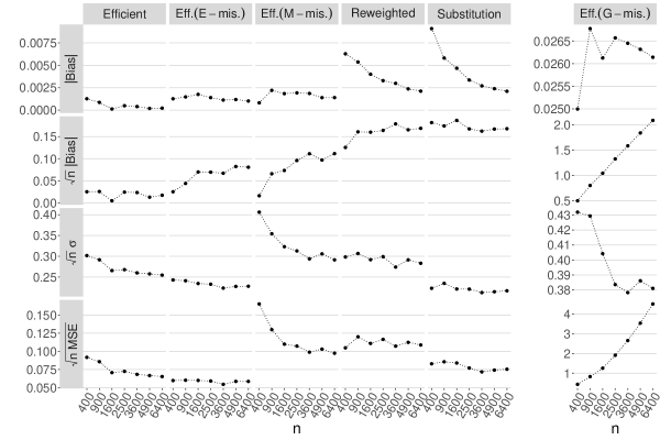
Figure 3: Statistics for the three key estimators (and variations thereof) of the direct effect under an IPS intervention $\delta=0.5$, across $1000$ Monte Carlo simulations for each of seven sample sizes.

Inspection of the mean-squared error, after scaling by $\sqrt{n}$, reveals that the substitution estimator and the efficient one-step estimator both display excellent, essentially equivalent performance when nuisance components are estimated using the highly adaptive lasso. The one-step estimator has slightly better performance, which seems to be driven by a better bias-variance trade-off. In contrast to the substitution estimator, the efficient one-step estimator carries the advantage of being double robust, allowing misspecification of either the outcome regression (denoted “M”) or the mediator-inclusive propensity score (denoted “E”). The robustness of the efficient estimator to the misspecification of these nuisance components — and the lack of robustness to the mediator-exclusive propensity score (denoted “G”) — are demonstrated in the last three rows of Table 1. Figure 3 visualizes the performance of the estimators, and their misspecified variants, in terms of both the MSE (as presented in Table 1) and its individual components, the bias and standard error. This comparison of the estimators reveals that the correctly-specified one-step efficient estimator displays excellent performance in terms of both bias and variance while its non-robust misspecified variant displays an asymptotic bias that grows with sample size. Interestingly, the one-step estimator with $e$ inconsistently estimated displayed better performance than the fully efficient version. This is possibly an idiosyncrasy of this simulation due to the fact that misspecification through an intercept-only model generates smaller variable weights. Altogether, these numerical investigations demonstrate the utility of the proposed estimators in settings where the nonparametric estimation of nuisance components is viable; moreover, in applied data analytic settings where this procedure may be of interest, the one-step efficient estimator is clearly preferable on account of its multiple robustness. All numerical studies of the estimators were performed using the implementations available in the medshift software package (Hejazi and Díaz, 2019) for the R language and environment for statistical computing (R Core Team, 2019).

6 Application

We now turn to considering a scenario in which the decomposition proposed in equation 5 and the proposed efficient estimator (16) may be used to estimate direct and indirect effects. To proceed, we take as example a simple data set from an observational study of the relationship between BMI and children’s behavior, distributed as part of the mma R package, available via the Comprehensive R Archive Network (https://CRAN.R-project.org/package=mma). The documentation of this data set describes it as a “database obtained from the Louisiana State University Health Sciences Center, New Orleans, by Dr. Richard Scribner [who] explored the relationship between BMI and kids behavior through a survey at children, teachers and parents in Grenada in 2014. This data set includes $691$ observations and $15$ variables.” In particular, we consider a modified version of this data set with all missing values removed, as these are irrelevant to the demonstration of the proposed methodology. In standard data analytic practice, we advocate for the use of the proposed methodology in tandem with a correction for missing data, such as imputation or weighting by inverse probability of censoring. (Carpenter et al., 2006; Vansteelandt et al., 2010; Seaman et al., 2012).

To demonstrate the assessment of the direct and indirect effect with this observational data set, we consider the effect of participation in a sports team on the BMI of children, taking several related covariates as mediators (including snacking, exercising, and overweight status) and all other collected covariates as potential confounders. As the intervention variable is binary, we frame our proposal in terms of an incremental propensity score intervention (Kennedy, 2018a), wherein the odds of participating in a sports team is increased by a factor of $\delta=2$ for each individual. Such a stochastic exposure regime may be interpreted as the introduction of a school program or policy that motivates children to opt in to participating in a sports team, doubling the odds of such voluntary participation.

6.1 Estimation Strategy

As noted in equation 5, the population intervention effect admits a decomposition in terms of components that allow estimation of the direct and indirect effects. We compute each of the components of the direct and indirect effects using appropriate estimators as follows

• for $\mathbb{E}\{Y(A,Z)\}=\mathbb{E}Y$, the natural value of the outcome under no intervention, the empirical mean in the sample serves as an efficient estimator;

• for $\mathbb{E}\{Y(A_{\delta},Z)\}=\theta(\delta)$, the mean outcome under an intervention altering the exposure mechanism but not the mediation mechanism, a one-step efficient estimator, denoted $\hat{\theta}(\delta)$, is proposed as equation 16 and made available via the medshift R package (Hejazi and Díaz, 2019);

• for $\mathbb{E}\{Y(A_{\delta})\}=\psi(\delta)$, the mean outcome under an intervention altering both the exposure and mediation mechanisms, a one-step efficient estimator, denoted $\hat{\psi}(\delta)$ in the sequel, is easily estimable using the npcausal R package (Kennedy, 2018b).

In the construction of estimators for $\theta(\delta)$ and $\psi(\delta)$, data adaptive nonparametric regression procedures are incorporated to allow the relevant nuisance parameters of each estimator to be computed in a flexible manner using various R packages. The npcausal package allows the estimator $\hat{\psi}(\delta)$ to be constructed using the ranger algorithm (Wright and Ziegler, 2015), an efficient and fast implementation of random forests (Breiman, 2001). In constructing $\hat{\theta}(\delta)$, the medshift package provides facilities for estimating nuisance parameters data adaptively via the Super Learner algorithm (van der Laan et al., 2007) for constructing ensemble learners through cross-validation, using its implementation in the sl3 package (Coyle et al., 2018). In particular, the Super Learner procedure was used to create a weighted ensemble of algorithms from a library including extreme gradient boosting via the xgboost package (Chen and Guestrin, 2016), with variants including 50, 100, and 300 boosting iterations; variants of random forests using 50, 100, and 500 trees; $L_{1}$-penalized lasso and $L_{2}$-penalized ridge GLMs via the glmnet package (Friedman et al., 2009); an elastic net GLM with equally weighted $L_{1}$ and $L_{2}$ penalization terms (also via glmnet); a main terms GLM; an intercept model; and the highly adaptive lasso (Benkeser and van der Laan, 2016), with 5–fold cross-validation and up to either 3-way or 5-way interaction terms, using the hal9001 package (Coyle and Hejazi, 2018).

6.2 Estimating the Direct and Indirect Effects

From the decomposition given in equation 5, the direct effect may be denoted $\beta(\delta)=\theta(\delta)-\mathbb{E}Y$. An estimator of the direct effect, $\hat{\beta}(\delta)$ may be expressed as a composition of estimators of its constituent parameters:

$$\hat{\beta}({\delta})=\hat{\theta}(\delta)-\frac{1}{n}\sum_{i=1}^{n}Y_{i}.$$

Using the estimation strategies previously outlined, we may construct an estimate of the direct effect through a straightforward application of the delta method, yielding both a point estimate and associated standard errors under our proposed stochastic intervention policy. Similarly, the indirect effect $\psi(\delta)-\theta(\delta)$ may be estimated as $\hat{\psi}(\delta)-\hat{\theta}(\delta)$. We provide both point estimates and associated inference under our proposed stochastic intervention policy in Table 2.

Parameter	Lower 95% CI	Estimate	Upper 95% CI
Direct Effect	-0.458	0.011	0.479
Indirect Effect	-0.672	-0.157	0.357

Table 2: Point estimates and 95% confidence intervals for the direct effect and indirect effect for an IPS intervention of $\delta=2$ applied to the data set from the mma R package.

From the estimates in Table 2, the conclusion may be easily drawn that there is little total effect of doubling the odds of participation in a sports team on the BMI of children, based on the data collected in the observational study made available in the mma R package. For reference, the marginal odds of participating in a sports team in the observed data are $0.69$, whereas the odds under the intervention considered are $1.38$. Based on the 95% confidence intervals around the point estimates, we cannot conclude that the proposed incremental propensity score intervention is sufficiently efficacious to decrease children’s BMI. However, the magnitude of the effects seem to be in the correct direction, with increased participation in a sports team causing a reduction of BMI of $0.157$ through changes in behaviors such as snacking and exercise. Using an approach similar to that demonstrated with this data set, the direct and indirect effects attributable to interventions with higher odds of participating in a sports team are easily estimable.

7 Discussion

We have proposed a novel mediation analysis based on the decomposition of the causal effect of a stochastic intervention on the population, focusing on two types of interventions: modified treatment policies and exponential tilting. Unlike the natural direct effect of Pearl (2001), identification of the (in)direct effect proposed here does not require cross-world counterfactual independencies, and is therefore achievable in an experimental setting randomizing both the exposure and the mediator.

We present results for stochastic interventions defined as a modified treatment policy and explicitly defined in terms of the post-intervention distribution (exponential tilting). In addition to the considerations about robustness and smoothness discussed in the present article, the choice between these two options may also be guided by the fact that modified treatment policies are more useful in practical settings as they can be used to inform feasible interventions.

Note that our effect decomposition and estimators allow for multivariate mediators. The interpretation of the (joint) indirect effect in this case is entirely context-dependent. For example, the multivariate mediators may represent an innately multivariate construct (e.g., a psychological construct such as personality, behavior, etc.) in this case the indirect effect could be interpreted as an effect through the construct (e.g., personality). Nonetheless, our approach does not require that the multivariate mediators are part of a single construct; the interpretation in these cases requires more care.

We assume that there is no mediator-outcome confounder affected by exposure. Point identification of natural (in)direct effects in the presence of such variables is not generally possible, and its partial identification is an area of active research (Robins and Richardson, 2010; Tchetgen and Phiri, 2014; Miles et al., 2015).

Lastly, for simplicity we focus on estimators constructed as solutions to the efficient influence function estimating equation; moreover, we have made implementations of each of the proposed estimators available in the free and open source medshift software package (Hejazi and Díaz, 2019) for the R language and environment for statistical computing (R Core Team, 2019). Alternative estimation strategies, such as targeted minimum loss-based estimation (van der Laan and Rubin, 2006; van der Laan and Rose, 2011, 2018), may have better performance than our propsoed estimators in finite samples. The development of such estimators will be the subject of future research and software development.

8 Proofs of results in the main document

8.1 Theorem 1

Proof We prove the result separately for exponential tilting and for modified treatment policies. First, let $A_{\delta}$ denote a variable drawn from the exponentially tilted distribution $g_{\delta}(a\mid w)$. We have

$$\mathbb{E}\{Y(A_{\delta},Z)\mid A_{\delta}=a,Z=z,W=w\} = \mathbb{E}\{Y(a,z)\mid A_{\delta}=a,Z=z,W=w\}$$

$$= \mathbb{E}\{Y(a,z)\mid Z=z,W=w\}$$

$$= \mathbb{E}\{Y(a,z)\mid A=a,Z=z,W=w\}$$

$$= m(z,a,w).$$

The first equality follows from the definition of $Y(A_{\delta},Z)$, the second equality follows because, by definition, $A_{\delta}\mbox{$\perp\!\!\!\perp$}Y(a,z)\mid(W,Z)$, and the third equality follows from A3. Finally, the fourth equality follows from the consistency implied by he NPSEM: $(A,Z)=(a,z)\rightarrow Y(a,z)=Y$.

Note that, by definition, $A_{\delta}\mbox{$\perp\!\!\!\perp$}Z\mid W$. Thus

$$\mathbb{E}\{Y(A_{\delta},Z)\}=\int_{\mathop{\mathrm{supp}}(g_{\delta})\times\mathop{\mathrm{supp}}(q)\times\mathop{\mathrm{supp}}(p)}m(z,a,w)r(z\mid w)g_{\delta}(a\mid w)p(w)d\nu(a,z,w),$$

where A2 ensures that $m(z,a,w)$ is defined in the integration set.

If the intervention is a modified treatment policies, such as our Example 1 where $A_{\delta}=d(A,W)$, then the proof proceeds as follows. First of all, we have $A\mbox{$\perp\!\!\!\perp$}Y(A_{\delta},Z)\mid(A_{\delta},Z,W)$, so that

$$\mathbb{E}\{Y(A_{\delta},Z)\mid A_{\delta}=a,A=a^{\prime},Z=z,W=w\}=m(z,a,w).$$

Integrating the above expression with respect to the joint density of $(A_{\delta},A,Z,W)$, and using

$$r(z\mid w)=\int_{\mathop{\mathrm{supp}}(g)}q(z\mid a^{\prime},w)g(a^{\prime}\mid w)d\nu(a^{\prime})$$

yields the desired result. ∎

8.2 DAGs compatible with A3

Lemma 5.

Define the non-parametric structural equation model in (1). If ($U_{A}\mbox{$\perp\!\!\!\perp$}U_{Y}$ and $U_{W}\mbox{$\perp\!\!\!\perp$}U_{Z}$ and $U_{Y}\mbox{$\perp\!\!\!\perp$}U_{Z}$) and either $U_{Y}\mbox{$\perp\!\!\!\perp$}U_{W}$ or $U_{A}\mbox{$\perp\!\!\!\perp$}U_{W}$, then A3 holds.

Proof For fixed $(a,z)$, let $Y(a,z)=f_{Y}(W,a,z,U_{Y})$. $(W,Z)$ d-separates $Y(a,z)$ from $A$ in Figures 4 and 5, concluding the proof of the lemma.

Figure 4: Directed Acyclic Graph for $U_{A}\mbox{$\perp\!\!\!\perp$}U_{Y}$ and $U_{W}\mbox{$\perp\!\!\!\perp$}U_{Z}$ and $U_{Y}\mbox{$\perp\!\!\!\perp$}U_{Z}$ and $U_{A}\mbox{$\perp\!\!\!\perp$}U_{W}$.

Figure 5: Directed Acyclic Graph for $U_{A}\mbox{$\perp\!\!\!\perp$}U_{Y}$ and $U_{W}\mbox{$\perp\!\!\!\perp$}U_{Z}$ and $U_{Y}\mbox{$\perp\!\!\!\perp$}U_{Z}$ and $U_{Y}\mbox{$\perp\!\!\!\perp$}U_{W}$.

∎

8.3 Theorem 2 and Lemmas 1 and 2

Proof In this proof we will use $\Theta(\mathbb{P})$ to denote a parameter as a functional that maps the distribution $\mathbb{P}$ in the model to a real number. We will assume that the measure $v$ is discrete so that integrals can be written as sums. The resulting influence function will also correspond to the influence function of a general measure $\nu$. For example, the true parameter value is given by

$$\theta(\delta)=\Theta(\mathbb{P})=\sum_{y,z,a,w}m(a,z,w)g_{\delta}(a\mid w)p(z,w).$$

Assume that $g_{\delta}$ is known. Then the non-parametric MLE of $\theta(\delta)$ is given by

$$\Theta(\mathbb{P}_{n}) =\sum_{y,z,a,w}y\mathbb{P}_{n}(y|a,z,w)g_{\delta}(a\mid w)\mathbb{P}_{n}(z,w)$$

$$=\sum_{y,z,a,w}y\frac{\mathbb{P}_{n}f_{y,a,z,w}}{\mathbb{P}_{n}f_{a,z,w}}g_{\delta}(a\mid w)\mathbb{P}_{n}f_{z,w},$$ (18)

where we remind the reader of the notation $Pf=\int fdP$. Here $f_{y,a,z,w}=I(Y=y,A=a,Z=z,W=w)$, $f_{a,z,w}=I(A=a,Z=z,W=w)$ , $f_{a,w}=I(A=a,W=w)$, $f_{z,w}=I(Z=z,W=w)$, and $I(\cdot)$ denotes the indicator function.

We will use the fact that the efficient influence function in a non-parametric model corresponds with the influence curve of the NPMLE. This is true because the influence curve of any regular estimator is also a gradient, and a non-parametric model has only one gradient. Appendix 18 of van der Laan and Rose (2011) shows that if $\hat{\Theta}(\mathbb{P}_{n})$ is a substitution estimator such that $\theta(\delta)=\hat{\Theta}(\mathbb{P})$, and $\hat{\Theta}(\mathbb{P}_{n})$ can be written as $\hat{\Theta}^{*}(\mathbb{P}_{n}f:f\in\mathcal{F})$ for some class of functions $\mathcal{F}$ and some mapping $B^{*}$, the influence curve of $\hat{\Theta}(\mathbb{P}_{n})$ is equal to

$$IC(\mathbb{P})(O)=\sum_{f\in\mathcal{F}}\frac{d\hat{\Theta}^{*}(\mathbb{P})}{d\mathbb{P}f}\{f(O)-\mathbb{P}f\}.$$

Applying this result to (18) with $\mathcal{F}=\{f_{y,a,z,w},f_{y,a,w},f_{a,w},f_{z,w},f_{w}\}$ gives an efficient influence function equal to $D^{Y}_{\eta,\delta}(o)+D^{Z,W}_{\eta,\delta}(o)-\theta(\delta)$. It remains to find the component $D^{A}_{\eta,\delta}(o)$ for each specific intervention. This component may be found as the IF of the estimator

$$\Theta(\mathbb{P}_{n})=\sum_{y,z,a,w}y\mathbb{P}(y|a,z,w)\hat{g}_{\delta}(a\mid w)\mathbb{P}(z,w),$$

where $\hat{g}_{\delta}$ is the MLE of $g_{\delta}$, obtained by substitution of the MLE of $g$.

The algebraic derivations described here are lengthy and not particularly illuminating, and are therefore omitted from the proof. ∎

8.4 Proof of Corollary 1

Proof In this proof we use the notation $\pi(w)=g(1\mid w)$. From the parameterization $e(a\mid z,w)=g(a\mid w)q(z\mid a,w)/r(z\mid w)$, note that

$$\phi(a,w)=\int m(a,z,w)\mathrm{d}\mathbb{P}(z\mid w).$$

Thus, $D^{A}_{\eta,\delta}(o)$ from Lemma 2 may be written as follows

$$D^{A}_{\eta,\delta}(o) =\sum_{t\in\{0,1\}}\frac{g_{\delta}(a\mid w)}{g(a\mid w)}\int m(t,z,w)\mathrm{d}\mathbb{P}(z\mid w)\{I(a=t)-g_{\delta}(t\mid w)\}$$

$$= \sum_{t\in\{0,1\}}\int m(t,z,w)\mathrm{d}\mathbb{P}(z\mid w)\left[a\frac{\pi_{\delta}(w)}{\pi(w)}\{t-g_{\delta}(t\mid w)\}+\right.$$

$$\left.(1-a)\frac{1-\pi_{\delta}(w)}{1-\pi(w)}\{1-t-g_{\delta}(t\mid w)\}\right]$$

Note that

$$\pi_{\delta}(w)\{t-g_{\delta}(t\mid w)\}=-\{1-\pi_{\delta}(w)\}\{1-t-g_{\delta}(t\mid w)\}=(2t-1)\pi_{\delta}(w)\{1-\pi_{\delta}(w)\}.$$

Thus,

$$D^{A}_{\eta,\delta}(o)= \sum_{t\in\{0,1\}}\int m(t,z,w)\mathrm{d}\mathbb{P}(z\mid w)(2t-1)\pi_{\delta}(w)\{1-\pi_{\delta}(w)\}\left[\frac{a}{\pi(w)}-\frac{1-a}{1-\pi(w)}\right]$$

$$= \frac{\pi_{\delta}(w)\{1-\pi_{\delta}(w)\}}{\pi(w)\{1-\pi(w)\}}\{a-\pi(w)\}\sum_{t\in\{0,1\}}\int m(t,z,w)\mathrm{d}\mathbb{P}(z\mid w)(2t-1)$$

since

$$\frac{\pi_{\delta}(w)\{1-\pi_{\delta}(w)\}}{\pi(w)\{1-\pi(w)\}}=\frac{\delta}{\{\delta\pi(w)+1-\pi(w)\}^{2}},$$

expanding the sum in $t$ concludes the proof. ∎

8.5 Proof of Theorem 3

Proof Let $\mathbb{P}_{n,j}$ denote the empirical distribution of the prediction set ${\cal V}_{j}$, and let $\mathbb{G}_{n,j}$ denote the associated empirical process $\sqrt{n/J}(\mathbb{P}_{n,j}-\mathbb{P})$. Note that

$$\hat{\theta}(\delta)=\frac{1}{J}\sum_{j=1}^{J}\mathbb{P}_{n,j}D_{\hat{\eta}_{j},\delta},\,\,\,\theta(\delta)=\mathbb{P}D_{\eta}.$$

Thus,

$$\sqrt{n}\{\hat{\theta}(\delta)-\theta(\delta)\}=\mathbb{G}_{n}\{D_{\eta,\delta}-\theta(\delta)\}+R_{n,1}(\delta)+R_{n,2}(\delta),$$

where

$$R_{n,1}(\delta)=\frac{1}{\sqrt{J}}\sum_{j=1}^{J}\mathbb{G}_{n,j}(D_{\hat{\eta}_{j},\delta}-D_{\eta,\delta}),\,\,\,R_{n,2}(\delta)=\frac{\sqrt{n}}{J}\sum_{j=1}^{J}\mathbb{P}\{D_{\hat{\eta}_{j},\delta}-\theta(\delta)\}.$$

It remains to show that $R_{n,1}(\delta)$ and $R_{n,2}(\delta)$ are $o_{P}(1)$. Theorem 5 together with the Cauchy-Schwartz inequality and assumption (i) of the theorem shows that $||R_{n,2}||_{\Delta}=o_{P}(1)$. For $||R_{n,1}||_{\Delta}$ we use empirical process theory to argue conditional on the training sample ${\cal T}_{j}$. In particular, Lemma 19.33 of van der Vaart (1998) applied to the class of functions ${\cal F}=\{D_{\hat{\eta}_{j},\delta}-D_{\eta,\delta}\}$ (which consists of one element) yields

$$E\left\{\big{|}\mathbb{G}_{n,j}(D_{\hat{\eta}_{j},\delta}-D_{\eta,\delta})\big{|}\,\bigg{|}\,{\cal T}_{j}\right\}\lesssim\frac{2C\log 2}{n^{1/2}}+||D_{\hat{\eta}_{j},\delta}-D_{\eta,\delta}||(\log 2)^{1/2}$$

By assumption (i), the left hand side is $o_{P}(1)$. Lemma 6.1 of Chernozhukov et al. (2018) may now be used to argue that conditional convergence implies unconditional convergence, concluding the proof.

∎

8.6 Proof of Theorem 4

Let $||f||_{\Delta}=\sup_{\delta\in\Delta}|f(\delta)|$. Let $\mathbb{P}_{n,j}$ denote the empirical distribution of the prediction set ${\cal V}_{j}$, and let $\mathbb{G}_{n,j}$ denote the associated empirical process $\sqrt{n/J}(\mathbb{P}_{n,j}-\mathbb{P})$. Note that

$$\hat{\theta}(\delta)=\frac{1}{J}\sum_{j=1}^{J}\mathbb{P}_{n,j}D_{\hat{\eta}_{j},\delta},\,\,\,\theta(\delta)=\mathbb{P}D_{\eta}.$$

Thus,

$$\sqrt{n}\{\hat{\theta}(\delta)-\theta(\delta)\}=\mathbb{G}_{n}\{D_{\eta,\delta}-\theta(\delta)\}+R_{n,1}(\delta)+R_{n,2}(\delta),$$

where

$$R_{n,1}(\delta)=\frac{1}{\sqrt{J}}\sum_{j=1}^{J}\mathbb{G}_{n,j}(D_{\hat{\eta}_{j},\delta}-D_{\eta,\delta}),\,\,\,R_{n,2}(\delta)=\frac{\sqrt{n}}{J}\sum_{j=1}^{J}\mathbb{P}\{D_{\hat{\eta}_{j},\delta}-\theta(\delta)\}.$$

The map $\delta\mapsto\bar{D}_{\eta,\delta}$ is Lipschitz, which implies that the class ${\cal F}=\{\bar{D}_{\eta,\delta}:\delta\in\Delta\}$ has bounded bracketing numbers (Theorem 2.7.11 of van der Vaart and Wellner, 1996). Therefore, $\cal F$ is Donsker and $\mathbb{G}_{n}\{D_{\eta,\delta}-\theta(\delta)\}\rightsquigarrow\mathbb{G}(\delta)$ in $\ell^{\infty}(\Delta)$.

It remains to show that $||R_{n,1}||_{\Delta}$ and $||R_{n,2}||_{\Delta}$ are $o_{P}(1)$. Theorem 6 together with the assumptions of the theorem and the Cauchy-Schwartz inequality, show that $||R_{n,2}||_{\Delta}=o_{P}(1)$. For $||R_{n,1}||_{\Delta}$ we use empirical process theory to argue conditional on the training sample ${\cal T}_{j}$. Let ${\cal F}_{n}^{j}=\{D_{\hat{\eta}_{j},\delta}-D_{\eta,\delta}:\delta\in\Delta\}$. Because the function $\hat{\eta}_{j}$ is fixed given the training data, we can apply Theorem 2.14.2 of van der Vaart and Wellner (1996) to obtain

$$E\left\{\sup_{f\in{\cal F}_{n}^{j}}|\mathbb{G}_{n,j}f|\,\,\bigg{|}\,\,{\cal T}_{j}\right\}\lesssim||F^{j}_{n}||\int_{0}^{1}\sqrt{1+N_{[\,]}(\epsilon||F_{n}^{j}||,{\cal F}_{n}^{j},L_{2}(\mathbb{P}))}\mathrm{d}\epsilon,$$

where $N_{[\,]}(\epsilon||F_{n}^{j}||,{\cal F}_{n}^{j},L_{2}(\mathbb{P}))$ is the bracketing number and we take $F_{n}^{j}=\sup_{\delta\in\Delta}|D_{\hat{\eta}_{j},\delta}-D_{\eta,\delta}|$ as an envelope for the class ${\cal F}_{n}^{j}$. Theorem 2.7.2 of van der Vaart and Wellner (1996) shows

$$\log N_{[\,]}(\epsilon||F_{n}^{j}||,{\cal F}_{n}^{j},L_{2}(\mathbb{P}))\lesssim\frac{1}{\epsilon||F_{n}^{j}||}.$$

This shows

$$||F^{j}_{n}||\int_{0}^{1}\sqrt{1+N_{[\,]}(\epsilon||F_{n}^{j}||,{\cal F}_{n}^{j},L_{2}(\mathbb{P}))}\mathrm{d}\epsilon \lesssim\int_{0}^{1}\sqrt{||F^{j}_{n}||^{2}+\frac{||F^{j}_{n}||}{\epsilon}}\mathrm{d}\epsilon$$

$$\leq||F^{j}_{n}||+||F^{j}_{n}||^{1/2}\int_{0}^{1}\frac{1}{\epsilon^{1/2}}\mathrm{d}\epsilon$$

$$\leq||F^{j}_{n}||+2||F^{j}_{n}||^{1/2}.$$

Since $||F^{j}_{n}||=o_{P}(1)$, this shows $\sup_{f\in{\cal F}_{n}^{j}}\mathbb{G}_{n,j}f=o_{P}(1)$ for each $j$, conditional on ${\cal T}_{j}$. and thus $||R_{n,1}||_{\Delta}=o_{P}(1)$, concluding the proof of the theorem.

9 Second order representation of the expectation of the EIF

Theorem 5.

Let $d(A,W)$ satisfy assumption A1. Denote $m_{d}(z,a,w)=m(z,d(a,w),w)$. Let $q_{1}(z\mid a,w)$ denote any density compatible with $\phi_{1}(a,w)$. That is, let $q_{1}$ be such that

$$\phi_{1}(a,w)=\int\frac{g_{1}(a\mid w)}{e_{1}(a\mid z,w)}m_{1,d}(z,a,w)q_{1}(z\mid a,w)d\nu(z),$$

and define $r_{1}=g_{1}q_{1}/e_{1}$. In this theorem we denote $\mathrm{d}\xi(w)=\mathrm{d}\mathbb{P}(w)$. We have

$$\mathbb{P}D_{\eta_{1},\delta}-\theta(\delta) = \int g_{\delta}\left(\frac{e}{e_{1}}-1\right)(m-m_{1})r\mathrm{d}\kappa\mathrm{d}\xi$$

$$+\int\frac{e}{e_{1}}(g_{\delta,1}-g_{\delta})(m-m_{1})r\mathrm{d}\kappa\mathrm{d}\xi$$

$$+\int m_{1,d}(r_{1}-r)(g-g_{1})\mathrm{d}\kappa\mathrm{d}\xi$$

Proof Note that

$$\mathbb{P}D^{Y}_{\eta_{1},\delta}+\mathbb{P}D^{Z,W}_{\eta,\delta}-\theta(\delta) = \int\frac{g_{\delta}}{e_{1}}(m-m_{1})er\mathrm{d}\kappa\mathrm{d}\xi-\int g_{\delta}(m-m_{1})r\mathrm{d}\kappa\mathrm{d}\xi$$

$$+\int\frac{e}{e_{1}}(g_{1,\delta}-g_{\delta})(m-m_{1})r\mathrm{d}\kappa\mathrm{d}\xi+\int m(g_{1,\delta}-g_{\delta})r\mathrm{d}\kappa\mathrm{d}\xi$$

$$= \int g_{\delta}\left(\frac{e}{e_{1}}-1\right)(m-m_{1})r\mathrm{d}\kappa\mathrm{d}\xi$$

$$+\int\frac{e}{e_{1}}(g_{1,\delta}-g_{\delta})(m-m_{1})r\mathrm{d}\kappa\mathrm{d}\xi$$

$$+\int(g_{1,\delta}-g_{\delta})m_{1}r\mathrm{d}\kappa\mathrm{d}\xi.$$

We have

$$\mathbb{P}D^{A}_{\eta_{1},\delta}=\mathbb{P}\left(\phi_{1}-\int\phi_{1}g_{1}d\nu\right)=\int(g-g_{1})m_{1,d}\frac{g_{1}q_{1}}{e_{1}}\mathrm{d}\kappa\mathrm{d}\xi.$$ (20)

Under A1, we can change variables in the following integral to obtain

$$\int(g_{1,\delta}-g_{\delta})m_{1}r\mathrm{d}\kappa\mathrm{d}\xi =\int(g_{1}-g)m_{1,d}r\mathrm{d}\kappa\mathrm{d}\xi$$

$$=\int(g_{1}-g)m_{1,d}\frac{gq}{e}\mathrm{d}\kappa\mathrm{d}\xi,$$

where we used the fact that $r(z\mid w)=g(a\mid w)q(z\mid a,w)/e(a\mid z,w)$. Adding this quantity in both sides of (20) we get

$$\mathbb{P}D^{A}_{\eta_{1},\delta}+\int(g_{1}-g)m_{1,d}r\mathrm{d}\kappa\mathrm{d}\xi = \int\frac{e_{1}q_{1}}{g_{1}}m_{1,d}(g_{1}-g)\mathrm{d}\kappa\mathrm{d}\xi$$

$$-\int\frac{eq}{g}m_{d}(g-g_{1})\mathrm{d}\kappa\mathrm{d}\xi$$

$$+\int\frac{eq}{g}(m_{d}-m_{1,d})(g-g_{1})\mathrm{d}\kappa\mathrm{d}\xi$$

$$= \int(\phi_{1}-\phi)(g-g_{1})\mathrm{d}\kappa\mathrm{d}\xi$$

$$+\int\frac{eq}{g}(m_{d}-m_{1,d})(g-g_{1})\mathrm{d}\kappa\mathrm{d}\xi.$$

∎

Theorem 6.

Define $c(w)=\{\int_{a}\exp(\delta a)g(a\mid w)\}^{-1}$, and let $c_{1}(w)$ be defined analogously. Let $b(a)=\exp(\delta a)$. Using the same notation as in Theorem 5, we have

$$\mathbb{P}D_{\eta_{1},\delta}-\theta(\delta) = \int g_{\delta}\left(\frac{e}{e_{1}}-1\right)(m-m_{1})r\mathrm{d}\kappa\mathrm{d}\xi$$

$$+\int\frac{e}{e_{1}}(g_{1,\delta}-g_{\delta})(m-m_{1})r\mathrm{d}\kappa\mathrm{d}\xi$$

$$+\int(g_{1,\delta}-g_{\delta})\{(m_{1}-m)r-(\phi_{1}-\phi)\}\mathrm{d}\kappa\mathrm{d}\xi$$

$$-\int\left\{(c_{1}-c)^{2}\int bg_{1}\phi\mathrm{d}\kappa\int bg\mathrm{d}\kappa\right\}\mathrm{d}\xi$$

$$+\int\left\{(c_{1}-c)\int b\phi(g-g_{1})\mathrm{d}\kappa\right\}\mathrm{d}\xi$$

Proof Let $q_{1}(z\mid a,w)$ be any density compatible with $\phi_{1}$. That is

$$\phi_{1}(a,w)=\int\frac{g_{1}(a\mid w)}{e_{1}(a\mid z,w)}m_{1}(a,z,w)q_{1}(z\mid a,w)\mathrm{d}\nu(z)$$

Note that display (9) is also valid here. Note also that

$$\int(g_{1,\delta}-g_{\delta})m_{1}r\mathrm{d}\kappa\mathrm{d}\xi=\int(g_{1,\delta}-g_{\delta})\phi\mathrm{d}\kappa\mathrm{d}\xi+\int(g_{1,\delta}-g_{\delta})\{(m_{1}-m)r-(\phi_{1}-\phi)\}\mathrm{d}\kappa\mathrm{d}\xi.$$

Note that $g_{1,\delta}(a\mid w)=c_{1}(w)b(a)g_{1}(a\mid w)$. We have

$$\mathbb{P}D_{\eta_{1}}^{A}+ \int(g_{\delta,1}-g_{\delta})\phi\mathrm{d}\xi$$

$$=\int\left\{\int\frac{g_{1,\delta}}{g_{1}}\phi g\mathrm{d}\kappa-\int\frac{g_{1,\delta}}{g_{1}}g\mathrm{d}\kappa\int\phi g_{1,\delta}\mathrm{d}\kappa+\int(g_{1,\delta}-g_{\delta})\phi\mathrm{d}\kappa\right\}\mathrm{d}\xi$$

$$=\int\left\{\frac{g_{1,\delta}}{g_{1}}g\phi\mathrm{d}\kappa-\int g_{\delta}\phi\mathrm{d}\kappa+\int g_{1,\delta}\phi\mathrm{d}\kappa\left[1-\int\frac{g_{1,\delta}}{g_{1}}g\mathrm{d}\kappa\right]\right\}\mathrm{d}\xi$$

$$=\int\left\{c_{1}\int b\phi g\mathrm{d}\kappa-c_{1}\int b\phi g\mathrm{d}\kappa+c_{1}\int bg\phi\mathrm{d}\kappa\int(c-c_{1})bg\mathrm{d}\kappa\right\}\mathrm{d}\xi$$

$$=\int(c_{1}-c)\left\{\int b\phi g\mathrm{d}\kappa-c_{1}\int bg_{1}\phi\mathrm{d}\kappa\int bg\mathrm{d}\kappa\right\}\mathrm{d}\xi$$

$$=\int(c_{1}-c)\left\{\int b\phi g\mathrm{d}\kappa-c\int bg_{1}\phi\mathrm{d}\kappa\int bg\mathrm{d}\kappa-(c_{1}-c)\int bg_{1}\phi\mathrm{d}\kappa\int bg\mathrm{d}\kappa\right\}\mathrm{d}\xi$$

$$=\int\left\{-(c_{1}-c)^{2}\int bg_{1}\phi\mathrm{d}\kappa\int bg\mathrm{d}\kappa+(c_{1}-c)\left[\int b\phi g\mathrm{d}\kappa-\int bg_{1}\phi\mathrm{d}\kappa\right]\right\}\mathrm{d}\xi$$ (21)

$$=\int\left\{-(c_{1}-c)^{2}\int bg_{1}\phi\mathrm{d}\kappa\int bg\mathrm{d}\kappa+(c_{1}-c)\int b\phi(g-g_{1})\mathrm{d}\kappa\right\}\mathrm{d}\xi,$$

where (21) follows from $c\int bg\mathrm{d}\kappa=1$ ∎

References

- Avin et al. (2005) Chen Avin, Ilya Shpitser, and Judea Pearl. Identifiability of path-specific effects. In IJCAI International Joint Conference on Artificial Intelligence, pages 357–363, 2005.
- Baron and Kenny (1986) Reuben M Baron and David A Kenny. The moderator–mediator variable distinction in social psychological research: Conceptual, strategic, and statistical considerations. Journal of personality and social psychology, 51(6):1173, 1986.
- Begun et al. (1983) Janet M Begun, WJ Hall, Wei-Min Huang, Jon A Wellner, et al. Information and asymptotic efficiency in parametric-nonparametric models. The Annals of Statistics, 11(2):432–452, 1983.
- Belloni et al. (2015) Alexandre Belloni, Victor Chernozhukov, Denis Chetverikov, and Ying Wei. Uniformly valid post-regularization confidence regions for many functional parameters in z-estimation framework. arXiv preprint arXiv:1512.07619, 2015.
- Benkeser and van der Laan (2016) David Benkeser and Mark van der Laan. The highly adaptive lasso estimator. In 2016 IEEE International Conference on Data Science and Advanced Analytics (DSAA), pages 689–696. IEEE, 2016.
- Bickel et al. (1997) Peter J Bickel, Chris AJ Klaassen, YA’Acov Ritov, and Jon A Wellner. Efficient and Adaptive Estimation for Semiparametric Models. Springer-Verlag, 1997.
- Breiman (1996) Leo Breiman. Stacked regressions. Machine learning, 24(1):49–64, 1996.
- Breiman (2001) Leo Breiman. Random forests. Machine learning, 45(1):5–32, 2001.
- Carpenter et al. (2006) James R Carpenter, Michael G Kenward, and Stijn Vansteelandt. A comparison of multiple imputation and doubly robust estimation for analyses with missing data. Journal of the Royal Statistical Society: Series A (Statistics in Society), 169(3):571–584, 2006.
- Chen and Guestrin (2016) Tianqi Chen and Carlos Guestrin. Xgboost: A scalable tree boosting system. In Proceedings of the 22nd acm sigkdd international conference on knowledge discovery and data mining, pages 785–794. ACM, 2016.
- Chernozhukov et al. (2013) Victor Chernozhukov, Denis Chetverikov, Kengo Kato, et al. Gaussian approximations and multiplier bootstrap for maxima of sums of high-dimensional random vectors. The Annals of Statistics, 41(6):2786–2819, 2013.
- Chernozhukov et al. (2016) Victor Chernozhukov, Denis Chetverikov, Mert Demirer, Esther Duflo, Christian Hansen, et al. Double machine learning for treatment and causal parameters. arXiv preprint arXiv:1608.00060, 2016.
- Chernozhukov et al. (2018) Victor Chernozhukov, Denis Chetverikov, Mert Demirer, Esther Duflo, Christian Hansen, Whitney Newey, and James Robins. Double/debiased machine learning for treatment and structural parameters. The Econometrics Journal, 21(1):C1–C68, 2018.
- Cole and Hernán (2002) Stephen R Cole and Miguel A Hernán. Fallibility in estimating direct effects. International journal of epidemiology, 31(1):163–165, 2002.
- Coyle and Hejazi (2018) Jeremy R Coyle and Nima S Hejazi. hal9001: The Scalable Highly Adaptive LASSO, 2018. URL https://github.com/tlverse/hal9001. R package version 0.2.1.
- Coyle et al. (2018) Jeremy R Coyle, Nima S Hejazi, Ivana Malenica, and Oleg Sofrygin. sl3: Modern pipelines for machine learning and Super Learning. https://github.com/tlverse/sl3, 2018. URL https://doi.org/10.5281/zenodo.1342294. R package version 1.1.0.
- Dawid (2000) A Philip Dawid. Causal inference without counterfactuals. Journal of the American Statistical Association, 95(450):407–424, 2000.
- Díaz and van der Laan (2012) Iván Díaz and Mark J van der Laan. Population intervention causal effects based on stochastic interventions. Biometrics, 68(2):541–549, 2012.
- Díaz and van der Laan (2013) Iván Díaz and Mark J van der Laan. Assessing the causal effect of policies: an example using stochastic interventions. The international journal of biostatistics, 9(2):161–174, 2013.
- Díaz and van der Laan (2018) Iván Díaz and Mark J van der Laan. Stochastic treatment regimes. In Targeted Learning in Data Science, pages 219–232. Springer, 2018.
- Didelez et al. (2006) Vanessa Didelez, A Philip Dawid, and Sara Geneletti. Direct and indirect effects of sequential treatments. In Proceedings of the Twenty-Second Conference on Uncertainty in Artificial Intelligence, pages 138–146. AUAI Press, 2006.
- Dudík et al. (2014) Miroslav Dudík, Dumitru Erhan, John Langford, Lihong Li, et al. Doubly robust policy evaluation and optimization. Statistical Science, 29(4):485–511, 2014.
- Friedman et al. (2009) Jerome Friedman, Trevor Hastie, and Rob Tibshirani. glmnet: Lasso and elastic-net regularized generalized linear models, 2009.
- Giné and Zinn (1984) Evarist Giné and Joel Zinn. Some limit theorems for empirical processes. The Annals of Probability, pages 929–989, 1984.
- Goldberger (1972) Arthur S Goldberger. Structural equation methods in the social sciences. Econometrica: Journal of the Econometric Society, pages 979–1001, 1972.
- Haneuse and Rotnitzky (2013) Sebastian Haneuse and Andrea Rotnitzky. Estimation of the effect of interventions that modify the received treatment. Statistics in Medicine, 2013.
- Hejazi and Díaz (2019) Nima S Hejazi and Iván Díaz. medshift: Causal mediation analysis for stochastic interventions in R, 2019. URL https://github.com/nhejazi/medshift. R package version 0.0.8.
- Imai et al. (2010) Kosuke Imai, Luke Keele, and Dustin Tingley. A general approach to causal mediation analysis. Psychological methods, 15(4):309, 2010.
- Kennedy (2018a) Edward H Kennedy. Nonparametric causal effects based on incremental propensity score interventions. Journal of the American Statistical Association, pages 1–12, 2018a.
- Kennedy (2018b) Edward H Kennedy. npcausal: Nonparametric causal inference methods, 2018b. URL https://github.com/ehkennedy/npcausal. R package version 0.1.0.
- Lok (2016) Judith J Lok. Defining and estimating causal direct and indirect effects when setting the mediator to specific values is not feasible. Statistics in medicine, 35(22):4008–4020, 2016.
- Lok (2019) Judith J Lok. Causal organic direct and indirect effects: closer to baron and kenny. arXiv preprint arXiv:1903.04697, 2019.
- Miles et al. (2015) Caleb H Miles, Phyllis Kanki, Seema Meloni, and Eric J Tchetgen Tchetgen. On partial identification of the pure direct effect. arXiv preprint arXiv:1509.01652, 2015.
- Newey (1994) Whitney K Newey. The asymptotic variance of semiparametric estimators. Econometrica: Journal of the Econometric Society, pages 1349–1382, 1994.
- Neyman (1923) J. Neyman. Sur les applications de la thar des probabilites aux experiences agaricales: Essay des principle (1923). excerpts reprinted (1990) in english (d. dabrowska and t. speed), trans. Statistical Science, 5:463–472, 1923.
- Nguyen et al. (2019) Trang Quynh Nguyen, Ian Schmid, and Elizabeth A Stuart. Clarifying causal mediation analysis for the applied researcher: Defining effects based on what we want to learn. arXiv preprint arXiv:1904.08515, 2019.
- Pearl (1995) Judea Pearl. Causal diagrams for empirical research. Biometrika, 82(4):669–688, 1995.
- Pearl (1998) Judea Pearl. Graphs, causality, and structural equation models. Sociological Methods & Research, 27(2):226–284, 1998.
- Pearl (2000) Judea Pearl. Causality: Models, Reasoning, and Inference. Cambridge University Press, Cambridge, 2000.
- Pearl (2001) Judea Pearl. Direct & indirect effects. In Proceedings of the 17th Conference in Uncertainty in Artificial Intelligence, UAI ’01, pages 411–420, San Francisco, CA, USA, 2001. Morgan Kaufmann Publishers Inc. ISBN 1-55860-800-1. URL http://dl.acm.org/citation.cfm?id=647235.720084.
- Pearl (2009) Judea Pearl. Myth, Confusion, and Science in Causal Analysis. Technical Report R-348, Cognitive Systems Laboratory, Computer Science Department University of California, Los Angeles, Los Angeles, CA, May 2009.
- Petersen et al. (2006) Maya L Petersen, Sandra E Sinisi, and Mark J van der Laan. Estimation of direct causal effects. Epidemiology, pages 276–284, 2006.
- Pfanzagl and Wefelmeyer (1985) J Pfanzagl and W Wefelmeyer. Contributions to a general asymptotic statistical theory. Statistics & Risk Modeling, 3(3-4):379–388, 1985.
- Popper (1934) K. R. Popper. The Logic of Scientific Discovery. Hutchinson, London, 1934.
- R Core Team (2019) R Core Team. R: A Language and Environment for Statistical Computing. R Foundation for Statistical Computing, Vienna, Austria, 2019. URL https://www.R-project.org/.
- Richardson and Robins (2013) Thomas S Richardson and James M Robins. Single world intervention graphs (swigs): A unification of the counterfactual and graphical approaches to causality. Center for the Statistics and the Social Sciences, University of Washington Series. Working Paper, 128(30):2013, 2013.
- Robins (1986) James M Robins. A new approach to causal inference in mortality studies with sustained exposure periods - application to control of the healthy worker survivor effect. Mathematical Modelling, 7:1393–1512, 1986.
- Robins and Greenland (1992) James M Robins and Sander Greenland. Identifiability and exchangeability for direct and indirect effects. Epidemiology, 3(0):143–155, 1992.
- Robins and Richardson (2010) James M Robins and Thomas S Richardson. Alternative graphical causal models and the identification of direct effects. Causality and psychopathology: Finding the determinants of disorders and their cures, pages 103–158, 2010.
- Robins et al. (2004) James M Robins, Miguel A Hernán, and UWE SiEBERT. Effects of multiple interventions. Comparative quantification of health risks: global and regional burden of disease attributable to selected major risk factors, 1:2191–2230, 2004.
- Rubin (1974) D. B. Rubin. Estimating Causal Effects of Treatments in Randomized & Nonrandomized Studies. Journal of Educational Psychology, 1974. URL http://www.eric.ed.gov/ERICWebPortal/detail?accno=EJ118470.
- Rudolph et al. (2017) Kara E Rudolph, Oleg Sofrygin, Wenjing Zheng, and Mark J Van Der Laan. Robust and flexible estimation of stochastic mediation effects: a proposed method and example in a randomized trial setting. Epidemiologic Methods, 7(1), 2017.
- Seaman et al. (2012) Shaun R Seaman, Ian R White, Andrew J Copas, and Leah Li. Combining multiple imputation and inverse-probability weighting. Biometrics, 68(1):129–137, 2012.
- Spirtes et al. (2000) Peter Spirtes, Clark N Glymour, Richard Scheines, David Heckerman, Christopher Meek, Gregory Cooper, and Thomas Richardson. Causation, prediction, and search. MIT press, 2000.
- Stitelman et al. (2010) Ori M Stitelman, Alan E Hubbard, and Nicholas P Jewell. The impact of coarsening the explanatory variable of interest in making causal inferences: Implicit assumptions behind dichotomizing variables. 2010.
- Stock (1989) James H Stock. Nonparametric policy analysis. Journal of the American Statistical Association, 84(406):567–575, 1989.
- Taubman et al. (2009) Sarah L Taubman, James M Robins, Murray A Mittleman, and Miguel A Hernán. Intervening on risk factors for coronary heart disease: an application of the parametric g-formula. International journal of epidemiology, 38(6):1599–1611, 2009.
- Tchetgen and Phiri (2014) Eric J. Tchetgen Tchetgen and Kelesitse Phiri. Bounds for pure direct effect. Epidemiology (Cambridge, Mass.), 25(5):775, 2014.
- Tchetgen Tchetgen and Shpitser (2012) Eric J Tchetgen Tchetgen and Ilya Shpitser. Semiparametric theory for causal mediation analysis: efficiency bounds, multiple robustness, and sensitivity analysis. Annals of Statistics, 40(3):1816, 2012.
- Tian (2008) Jin Tian. Identifying dynamic sequential plans. In Proceedings of the Twenty-Fourth Conference on Uncertainty in Artificial Intelligence, pages 554–561. AUAI Press, 2008.
- van der Laan (2017) Mark J van der Laan. A generally efficient targeted minimum loss based estimator based on the highly adaptive lasso. The International Journal of Biostatistics, 13(2), 2017.
- van der Laan and Benkeser (2018) Mark J van der Laan and David Benkeser. Highly adaptive lasso (hal). In Targeted Learning in Data Science, pages 77–94. Springer, 2018.
- van der Laan and Petersen (2008) Mark J van der Laan and Maya L Petersen. Direct effect models. The international journal of biostatistics, 4(1), 2008.
- van der Laan and Robins (2003) Mark J van der Laan and James M Robins. Unified Methods for Censored Longitudinal Data and Causality. Springer, New York, 2003.
- van der Laan and Rose (2011) Mark J van der Laan and Sherri Rose. Targeted Learning: Causal Inference for Observational and Experimental Data. Springer, New York, 2011.
- van der Laan and Rose (2018) Mark J van der Laan and Sherri Rose. Targeted Learning in Data Science: Causal Inference for Complex longitudinal Studies. Springer, New York, 2018.
- van der Laan and Rubin (2006) Mark J van der Laan and Daniel Rubin. Targeted maximum likelihood learning. The International Journal of Biostatistics, 2(1), 2006.
- van der Laan et al. (2007) M.J. van der Laan, E. Polley, and A. Hubbard. Super learner. Statistical Applications in Genetics & Molecular Biology, 6(25):Article 25, 2007.
- van der Vaart (1998) A. W. van der Vaart. Asymptotic Statistics. Cambridge University Press, 1998.
- van der Vaart (2002) Aad van der Vaart. Semiparameric statistics. Lectures on Probability Theory and Statistics, pages 331–457, 2002.
- van der Vaart (1991) Aad W van der Vaart. On differentiable functionals. Annals of Statistics, 19:178–204, 1991.
- van der Vaart and Wellner (1996) Aad W van der Vaart and Jon A Wellner. Weak Convergence and Emprical Processes. Springer-Verlag New York, 1996.
- VanderWeele et al. (2014) Tyler J VanderWeele, Stijn Vansteelandt, and James M Robins. Effect decomposition in the presence of an exposure-induced mediator-outcome confounder. Epidemiology (Cambridge, Mass.), 25(2):300, 2014.
- Vansteelandt and Daniel (2017) Stijn Vansteelandt and Rhian M Daniel. Interventional effects for mediation analysis with multiple mediators. Epidemiology (Cambridge, Mass.), 28(2):258, 2017.
- Vansteelandt and VanderWeele (2012) Stijn Vansteelandt and Tyler J VanderWeele. Natural direct and indirect effects on the exposed: effect decomposition under weaker assumptions. Biometrics, 68(4):1019–1027, 2012.
- Vansteelandt et al. (2010) Stijn Vansteelandt, James Carpenter, and Michael G Kenward. Analysis of incomplete data using inverse probability weighting and doubly robust estimators. Methodology, 2010.
- Vansteelandt et al. (2012) Stijn Vansteelandt, Maarten Bekaert, and Theis Lange. Imputation strategies for the estimation of natural direct and indirect effects. Epidemiologic Methods, 1(1):131–158, 2012.
- Wright and Ziegler (2015) Marvin N Wright and Andreas Ziegler. Ranger: a fast implementation of random forests for high dimensional data in c++ and r. arXiv preprint arXiv:1508.04409, 2015.
- Wright (1921) Sewall Wright. Correlation and causation. Journal of agricultural research, 20(7):557–585, 1921.
- Wright (1934) Sewall Wright. The method of path coefficients. The annals of mathematical statistics, 5(3):161–215, 1934.
- Young et al. (2014) Jessica G Young, Miguel A Hernán, and James M Robins. Identification, estimation and approximation of risk under interventions that depend on the natural value of treatment using observational data. Epidemiologic methods, 3(1):1–19, 2014.
- Zheng and van der Laan (2017) Wenjing Zheng and Mark van der Laan. Longitudinal mediation analysis with time-varying mediators and exposures, with application to survival outcomes. Journal of causal inference, 5(2), 2017.
- Zheng and van der Laan (2011) Wenjing Zheng and Mark J van der Laan. Cross-validated targeted minimum-loss-based estimation. In Targeted Learning, pages 459–474. Springer, 2011.
- Zheng and van der Laan (2012) Wenjing Zheng and Mark J van der Laan. Targeted maximum likelihood estimation of natural direct effects. The international journal of biostatistics, 8(1):1–40, 2012.