Dynamic Loop Scheduling Using
MPI Passive-Target Remote Memory Access

Abstract

Scientific applications often contain large computationally-intensive parallel loops. Loop scheduling techniques aim to achieve load balanced executions of such applications. For distributed-memory systems, existing dynamic loop scheduling (DLS) libraries are typically MPI-based, and employ a master-worker execution model to assign variably-sized chunks of loop iterations. The master-worker execution model may adversely impact performance due to the master-level contention. This work proposes a distributed chunk-calculation approach that does not require the master-worker execution scheme. Moreover, it considers the novel features in the latest MPI standards, such as passive-target remote memory access, shared-memory window creation, and atomic read-modify-write operations. To evaluate the proposed approach, five well-known DLS techniques, two applications, and two heterogeneous hardware setups have been considered. The DLS techniques implemented using the proposed approach outperformed their counterparts implemented using the traditional master-worker execution model.

Keywords

Dynamic loop scheduling; Distributed-memory systems; Master-worker execution model; MPI; Passive-target remote memory access.

1 Introduction

Over the past decade, the increasing demand for computational power of scientific applications played a significant role in the development of modern high performance computing (HPC) systems. The advancements of modern HPC systems at both, hardware and software levels, raise questions regarding the benefits of these advantages for successful algorithms and techniques proposed in the past. Algorithms and techniques may, therefore, need to be revisited and re-evaluated to fully leverage the capabilities of modern HPC systems. Dynamic loop scheduling (DLS) techniques are important examples of successful scheduling techniques proposed over the years. The DLS techniques are critical for scheduling parallel loops that are the main source of parallelism in scientific applications [1]. A large body of work on DLS was introduced between the late 1980’s and the early 2000’s [2, 3, 4, 5, 6, 7, 8]. These DLS techniques were used in several scientific applications to achieve a load balanced execution of loop iterations. Several factors can hinder such a load balanced execution, and consequently, degrade applications’ performance. Specifically, problem characteristics, non-uniform input data sets, as well as algorithmic and systemic variations lead to different execution times of each loop iteration. The DLS techniques are designed to mitigate load imbalance due to the aforementioned factors.

Dynamic loop self-scheduling-based techniques such as, self-scheduling (SS)[2], guided self-scheduling (GSS) [3], trapezoid self-scheduling (TSS) [4], factoring (FAC) [5], and weighted factoring (WF) [6], constitute an important category of DLS techniques. The distinguishing aspect of loop self-scheduling is that whenever a processing element becomes available and requests work, it obtains a collection of loop iterations (called a chunk) from a central work queue. Each DLS technique uses a certain function to calculate chunk sizes.

Several implementations of self-scheduling-based techniques [9, 10, 11, 12, 8] employ the master-worker execution model, and use the classical two-sided MPI communication model. In the master-worker execution model, a processing element (called master) holds all the information required to calculate the chunks and serves work requests from other processing elements (called workers). Workers request new chunks once they become available, according to the self-scheduling principle. The master-worker execution model highlights an important performance-relevant detail concerning the implementation of self-scheduling-based techniques; it centralizes the chunk-calculations at the master. This centralization renders the master process a performance bottleneck in three scenarios: (1) the master process has a decreased processing capabilities; this may happen in heterogeneous systems, (2) the master process receives a large number of concurrent work requests; this may happen in large-scale distributed-memory systems, and (3) a combination of (1) and (2) may be the case when executing on large-scale heterogeneous systems.

The current work proposes an approach to address the first execution scenario described above. Intuitively, this scenario can be avoided by mapping the master process to the processing element with the highest processing capabilities. However, such a mapping may not always be guaranteed or feasible. For instance, system variations during applications’ execution may adversely affect the computation or the communication capabilities of the master leading to performance degradation.

The MPI-2 standard [13] introduced remote memory access (RMA) semantics that were seldomly adopted in scientific applications because they had several issues [14]. For instance, the unrestricted allocation of exposed-memory regions makes the efficient implementation of one-sided functions extremely difficult. The MPI RMA model was significantly revised in the MPI-3 standard and more performance-capable RMA semantics were introduced [15, 16]. For instance, MPI_Win_Allocate was introduced to restrict the memory allocation and to allow more efficient MPI one-sided implementations. The performance assessment of MPI RMA-based approaches has recently gained increased attention for different scientific applications [17, 18, 19].

The present work proposes a novel approach for developing DLS techniques to execute scientific applications on distributed-memory systems. The proposed approach distributes the chunk-calculation of the DLS techniques among all processing elements. Moreover, the proposed approach is implemented using the recent features offered by the MPI-3 standard, such as passive-target synchronization, shared-memory window creation, and atomic read-modify-write operations. The present work is significant for improving the performance of various scientific applications, such as N-body simulations [20], Monte-Carlo simulations, and computational fluid dynamics [7], that employ DLS techniques on heterogeneous and large scale modern HPC systems. Moreover, the present work provides insights for improving existing DLS libraries [10, 11] such that they take advantage of modern HPC systems by exploiting the remote direct memory access (RDMA) capabilities of modern interconnection networks.

The main contributions of this work are: (1) Proposal and implementation of five DLS techniques with distributed chunk-calculation for distributed-memory systems. (2) Evaluation of the benefit of using MPI one-sided communication and passive-target synchronization mode to implement the DLS techniques: SS [2], GSS [3], TSS [4], FAC [5], and WF [6] against other existing approaches [10, 11, 21].

The remainder of this work is organized as follows. Section 2 contains a review of the selected DLS techniques, as well as of the relevant research efforts on the different implementation approaches of DLS techniques for distributed-memory systems. Also, the background on the MPI RMA model is presented in Section 2. The proposed distributed chunk-calculation approach and its execution model are introduced in Section 3. The design of experiments and the experimental results are discussed in Sections 4 and 5, respectively. The conclusions and the potential future work are outlined in Section 6.

2 Background and Related Work

Loop Scheduling

Loops are the richest source of parallelism in scientific applications [1]. Computationally-intensive scientific applications spend most of their execution time in large loops. Therefore, efficient scheduling of loop iterations benefits scientific applications’ performance. In the current work, five well-known DLS techniques: self-scheduling (SS) [2], guided self-scheduling (GSS) [3], trapezoid self-scheduling (TSS) [4], factoring FAC [5], and weighted factoring (WF) [6] are considered. These techniques are considered due to their competitive performance in different applications, and due to the fact that they are at the basis of other DLS techniques. For instance, trapezoid factoring self-scheduling (TFSS) [22] is based on TSS and FAC, while adaptive weighted factoring (AWF) [7] and its variants [23] are derived from FAC.

Table 1: Notation used in the present work

Symbol	Description
$N$	Total number of loop iterations
$P$	Total number of processing elements
$S$	Total number of scheduling steps
$B$	Total number of scheduling batches
$i$	Index of current scheduling step, $0\leq i\leq S-1$
$b$	Index of currently scheduled batch, $0\leq b\leq B-1$
$R_{i}$	Remaining loop iterations after $i$-th scheduling step
$S_{i}$	Scheduled loop iterations after $i$-th scheduling step $S_{i}+R_{i}=N$
$lp_{\text{start}}$	Index of currently executed loop iteration, $0\leq lp_{\text{start}}\leq N-1$
$K_{0}$	Size of the largest chunk
$K_{S-1}$	Size of the smallest chunk
$K_{i}$	Chunk size calculated at scheduling step $i$
$p_{j}$	Processing element $j$, $0\leq j\leq P-1$
$Wp_{j}$	Relative weight of processing element $j$, $0\leq j\leq P-1$, $\sum_{j=0}^{P-1}Wp_{j}=P$
$\sigma$	Standard deviation of the loop iterations’ execution times
$\mu$	Mean of the loop iterations’ execution times
$T_{\text{p}}$	Parallel execution time of the entire application
$T_{\text{p}}^{\text{loop}}$	Parallel execution time of the application’s parallelized loops

The common aspect of all selected DLS techniques is that new chunks of iterations are assigned to processing elements once they become available and request work. However, each of these DLS techniques employs a different function to calculate the size of the chunk to be assigned.

The notation used in the present work is given in Table 1. In the SS [2] technique, the assigned chunk, $K_{i}$, is always 1 loop iteration. Due to the fine-grained partitioning of the loop iterations, SS can achieve a highly load balanced execution. However, it incurs a high scheduling overhead. GSS [3], TSS [4], and FAC [5] outperform SS in terms of scheduling overhead, by assigning chunks of decreasing size. In each scheduling step $i$, GSS uses a non-linear function to calculate the chunk sizes. It divides the remaining loop iterations, $R_{i}$, by the total number of processing elements, $P$.

TSS [4] employs a simplistic linear function to calculate the decreasing chunk sizes using a fixed decrement. This linearity results in low scheduling overhead in each scheduling step.

FAC [5] schedules the loop iterations in batches of $P$ equally-sized chunks. The initial chunk size of FAC is smaller than the initial chunk size of GSS. If more time-consuming loop iterations exist at the beginning of the loop, GSS may not balance their execution as efficiently as FAC. Unlike GSS and TSS, which calculate the chunks deterministically, the chunk-calculation in FAC evolved from comprehensive probabilistic analyses. To calculate an optimal chunk size, FAC requires prior knowledge about the standard deviation, $\sigma$, of loop iterations’ execution times and their mean execution time $\mu$. A practical implementation of FAC, denoted FAC2, does not require $\mu$ and $\sigma$, and assigns half of the remaining work in every batch [5]. FAC2 evolved from the probabilistic analysis that gave birth to FAC, and is considered in the current work.

WF [6] uses the FAC function to calculate the batch size. However, the processing elements execute variably-sized chunks of this batch according to their relative weights. The processor weights, $Wp_{j}$, are determined prior to applications’ execution and do not change during the execution. The chunk-calculation function of each technique is shown in Table 2.

Table 2: Chunk-calculation per loop self-scheduling technique

Technique	Chunk-calculation
STATIC	$K_{i}=\left\lceil\frac{N}{P}\right\rceil$.
SS	$K_{i}=1$.
GSS	$K_{i}=\left\lceil\frac{R_{i}}{P}\right\rceil$, $R_{0}=N$.
TSS	$K_{i}=K_{i-1}-\left\lfloor\frac{K_{0}-K_{S-1}}{S-1}\right\rfloor$, where $S=\left\lceil\frac{2\cdot N}{K_{0}+K_{S-1}}\right\rceil$, and $K_{0}=\left\lceil\frac{N}{2\cdot P}\right\rceil\-\-,K_{S-1}=1$.
FAC2	$K_{i}=\left\{\begin{array}[]{ll}\left\lceil\frac{R_{i}}{2\cdot P}\right\rceil,&\text{if}\ i\-\-\mod P=0\\ R_{i-1},&\text{otherwise.}\end{array}\right.$
WF	$K_{i}=\left\lceil Wp_{j}\times K_{i}^{\text{FAC2}}\right\rceil$.

Related Work

Chronopoulos et al. introduced a distributed approach for implementing self-scheduling techniques (DSS) [24]. The goal was to improve the performance of the self-scheduling techniques on heterogeneous and distributed-memory resources. The proposed scheme was based on the master-worker execution model, similar to the one illustrated in Figure 1(a), and was implemented using the classical two-sided MPI communication. The main idea was to enable the master to consider the speed of the processing elements and their loads when assigning new chunks. Chronopoulos et al. later enhanced the performance of the DSS scheme using a hierarchical master-worker model, and proposed the hierarchical distributed self-scheduling (HDSS) [22] that was similar to the one illustrated in Figure 1(b). DSS and HDSS assume a dedicated master configuration in which the master processing element is reserved for handling the worker requests. Such a configuration may enhance the scalability of the proposed self-scheduling schemes. However, it results in low CPU utilization of the master. HDSS [22] suggested deploying the global-master and the local-master on one physical computing node that has multiple processing elements to overcome the low CPU utilization of the master (cf. Figure 1(b)).

Cariño et al. proposed a load balancing (LB) tool that integrated several DLS techniques [11]. At the conceptual level, the LB tool is based on a single-level master-worker execution model (cf. Figure 1(a)). However, it did not assume a dedicated-master. It introduced the breakAfter parameter which is user-defined and indicates how many iterations the master should execute before serving pending worker requests. This parameter is required for dividing the time of the master between computation and servicing of worker requests. The optimal value of this parameter is application- and system-dependent. The LB tool also employed the classical two-sided MPI communication.

Banicescu et al. proposed a dynamic load balancing library (DLBL) for cluster computing [10]. The DLBL is based on a parallel runtime environment for multicomputer applications (PREMA) [25]. Even though the DLBL was the first library to utilize MPI one-sided communication, the active message synchronization offered by PREMA required a master-worker model. In DLBL, the master expects work requests. Then, it calculates the size of the chunk to be assigned and, subsequently, calls a handler function on the worker side. The worker is responsible for obtaining the data of the new chunk from the master without any further involvement from the master.

Hierarchical loop scheduling (HLS) [12] was one of the earliest efforts to utilize a hybrid MPI and OpenMP programming model to implement DLS techniques. HLS employed a hierarchical master-worker execution model, and was implemented using the classical two-sided MPI communication and OpenMP threads. Unlike HDSS [22], HLS distributes the local masters across all physical computing nodes (cf. Figure 1(c)). The local masters communicate with the global master to request a new chunk when they have no more iterations to distribute between their workers. The main limitation of HLS is that the OpenMP worker threads distribute the work using the #pragma omp parallel region without the explicit use of the nowait clause. This incurs implicit local synchronization at the OpenMP level on local masters.

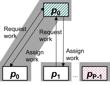
(a) Conventional master-worker execution model

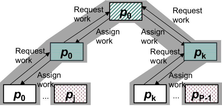
(b) Global and local masters are located on a single physical compute node

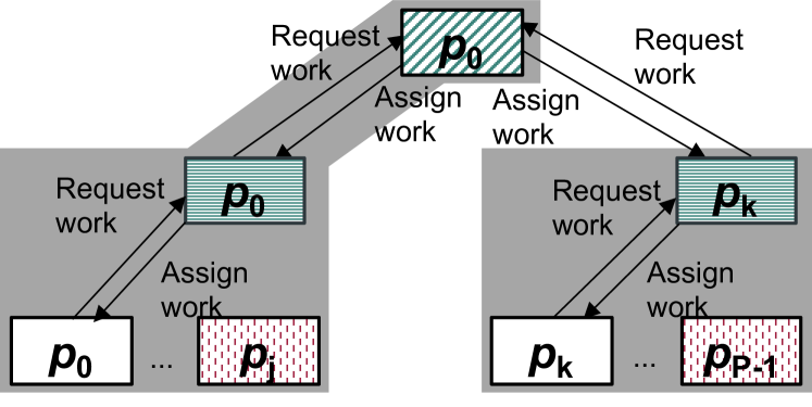
(c) Local masters are distributed across multiple physical compute nodes

Figure 1: Variants of the master-worker execution model as reported in the literature. Replication of certain processing elements is just to indicate their double role where the master participates in the computation as a worker.

MPI RMA Model

In MPI, the memory of each process is by default private, and other processes cannot directly access it. The MPI RMA model allows MPI processes to publicly expose different regions of their memory, called windows. One MPI process (origin) can directly access a memory window without any involvement of the other (target) process that owns the window. The MPI RMA has two synchronization modes: passive- and active-target. In the active-target synchronization, the target process determines the time boundaries, called epochs, when its window can be accessed. In the passive-target synchronization, the target process has no time limits when its window can be accessed. The present work focuses on the passive-target synchronization because it requires a minimal amount of synchronization, and it efficiently allows the greatest overlap of computation and communication. Moreover, it yields the development of DLS techniques for distributed-memory systems to be very similar to their original implementations for shared-memory systems.

3 The Proposed Approach

The main challenge to design a distributed chunk-calculation approach is associated with the chunk-calculation functions of the DLS techniques. To calculate the current chunk to be assigned, these functions (except for SS) require either the value of the remaining loop iterations $R_{i}$ or the value of the previous chunk $K_{i-1}$ (cf. Table 2). Therefore, the chunks have to be calculated in a sequential manner, i.e., two chunks cannot be calculated simultaneously because the values of $R_{i}$ and $K_{i-1}$ change after each chunk-calculation. This serialization perfectly fits any master-worker-based execution approach because the master serves one request at a time, and consequently, the chunk-calculation can be performed in a centralized and sequential fashion.

The approach proposed in this work introduces certain transformations of the respective chunk-calculation functions from Table 2, such that the chunk-calculation depends only on the index of the last scheduling step $i$. These transformations are shown below in Equations 1-3.

GSS: $$\ \ \ K^{\prime}_{i}=\left\lceil\left(\frac{P-1}{P}\right)^{i}\cdot\frac{N}{P}\right\rceil$$ (1)

TSS: $$\ \ \ K^{\prime}_{i}=K_{0}-i\cdot\left\lfloor\frac{K_{0}-K_{S-1}}{S-1}\right\rfloor$$ (2)

FAC2: $$\ \ \ K^{\prime}_{i}=\left\lceil\left(\frac{1}{2}\right)^{i_{\text{new}}}\cdot\frac{N}{P}\right\rceil,\ \ i_{\text{new}}=\left\lfloor\frac{i}{P}\right\rfloor+1$$ (3)

For GSS and FAC, the transformations were already introduced in the literature [5]. For TSS, the mathematical derivation of the transformation is as follows. Given that $S$, $K_{0}$, and $K_{S-1}$ are constants, the TSS equation in Table 2 can be represented as follows.

$$K_{i}=K_{i-1}-C,\text{where C is a constant value.}$$ (4)

$$C=\lfloor\frac{K_{0}-K_{S-1}}{S-1}\rfloor$$ (5)

Calculating $K_{1}$, $K_{2}$, $K_{3}$, $...$ $K_{i}$ using Equation 4

$$K_{1}=K_{0}-C$$ (6)

$$K_{2}=K_{1}-C=(K_{0}-C)-C=K_{0}-2\cdot C$$ (7)

$$K_{3}=K_{2}-C=(K_{0}-2\cdot C)-C=K_{0}-3\cdot C$$ (8)

$$K_{i}=K_{0}-i\cdot C$$ (9)

$$K_{i}=K_{0}-i\cdot\lfloor\frac{K_{0}-K_{S-1}}{S-1}\rfloor=K^{\prime}_{i}$$ (10)

WF uses the chunk-calculation function of FAC and can naturally inherit the transformed FAC function.

The proposed approach uses Equations 1-3 to distribute the chunk-calculation across all processing elements. Thus, only one processing element (called coordinator) stores index of the last scheduling step $i$ and the index of the last scheduled loop iteration $lp_{\text{start}}$.

Figure 2 illustrates the main steps of the proposed distributed chunk-calculation approach:
Step 1. the processing element $p_{j}$ obtains a copy of the last scheduling step index, $i$, and atomically increments the global $i$ by one.
Step 2. $p_{j}$ only uses its local copy of $i$ (before the increment) to calculate $K_{i}$ with the function of the selected DLS technique (Equations 1-3).
Step 3. $p_{j}$ obtains a copy of the last loop index start, $lp_{\text{start}}$, and atomically accumulates the size of the calculated chunk, $K_{i}$, into it.
Finally, $p_{j}$ executes loop iterations between $lp_{\text{start}}$ (before accumulation) and min($lp_{\text{start}}+K_{i}$, $N$). The atomic operations in Steps 1 and 3 guarantee the exclusive access to $i$ and $lp_{\text{start}}$.

The MPI RMA model provides the necessary function calls that can be used in the implementation of the proposed approach. For instance, the coordinator MPI process can use MPI_Win_create to expose the shared variables, such as $i$ and $lp_{\text{start}}$, to all other MPI processes. The passive-target synchronization mode (MPI_Win_lock(MPI_LOCK_SHARED)) can be used with certain MPI atomic operations, such as MPI_Get_accumulate, to grant the exclusive access to $i$ and $lp_{\text{start}}$ by all MPI processes. For more information regarding the implementation, the reader is referred to the code that is developed under the LGPL license and available online [26].

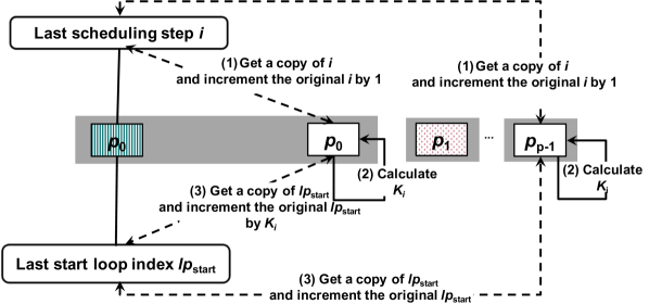
Figure 2: The proposed distributed chunk-calculation approach using MPI RMA and passive-target synchronization.

Figure 3 illustrates the DLS execution using the proposed distributed chunk-calculation approach. The calculation of chunks $K_{0}$ and $K_{1}$ is distributed between processors $p_{0}$ and $p_{1}$. The time required to calculate $K_{0}$ overlaps with the time taken to calculate $K_{1}$. In the traditional master-worker execution model, there is no such overlap since all the chunk calculations are centralized and performed by the master in sequence. The time required to serve the first work request (including chunk-calculation and chunk-assignment) delays the second work request. Moreover, the time required to serve the work requests is proportional to the processing capabilities of the master processor, which may result in additional delays as discussed in Section 1.

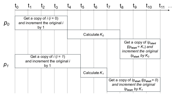
Figure 3: Schematic execution of the proposed distributed chunk-calculation approach on two processors that calculate one chunk each.

The proposed distributed chunk-calculation approach may result in a different ordering of assigning and executing loop iterations compared to the traditional master-worker execution model. For instance, when GSS is the chosen scheduling technique in Figure 3 and $N=10$, $p_{0}$ obtains a local copy of the last scheduling index $i=0$ at $t_{4}$. Also, $p_{1}$ obtains at $t_{5}$ a local copy of the last scheduling index $i=1$. Both, $p_{0}$ and $p_{1}$ use their copies of $i$ and calculate $K_{0}=5$ and $K_{1}=3$, respectively. The proposed approach does not guarantee that $p_{0}$ and $p_{1}$ will execute loop iterations from $lp_{\text{start}}=0$ to $lp_{\text{start}}=4$ and $lp_{\text{start}}=5$ to $lp_{\text{start}}=7$. Figure 3 shows the case when the chunk-calculation on $p_{0}$ is longer than on $p_{1}$, and results in assigning $p_{1}$, loop iterations between $lp_{start}=0$ and $lp_{start}=2$, while $p_{0}$ is assigned loop iterations between $lp_{\text{start}}=3$ and $lp_{\text{start}}=7$. Given that DLS techniques address, by design, independent loop iterations with no restrictions on the monotonicity of the loop execution, the proposed approach does not affect the correctness of the loop execution.

4 Design and Setup of Experiments

In the present work, the performance of two different implementations of DLS techniques is assessed. The first implementation, denoted One_Sided_DLS, employs the proposed distributed chunk-calculation approach and uses one-sided MPI communication in the passive-target synchronization mode. The second implementation, denoted Two_Sided_DLS, employs a master-worker model and uses the two-sided MPI communication. Both implementations assume a non-dedicated coordinator (or a non-dedicated master) processing element.

Selected Applications

Two computationally-intensive parallel applications are considered in this study. The first application, called PSIA [27], uses a parallel version of the well-known spin-image algorithm (SIA) [28]. SIA converts a 3D object into a set of 2D images. The generated 2D images can be used as descriptive features of the 3D object. The second application calculates the Mandelbrot set [29]. The Mandelbrot set is used to represent geometric shapes that have the self-similarity property at various scales. Studying such shapes is important and of interest in different domains, such as biology, medicine, and chemistry [30].

Both applications contain a single large parallel loop that dominates their execution times. Dynamic and static distributions of the most time-consuming parallel loop across all processing elements may enhance applications’ performance. The pseudocodes of both applications listed in Algorithm 1 and 2.

1 spinImagesKernel (W, B, S, OP, M);

Inputs : W: image width, B: bin size, S: support angle, OP: list of 3D points, M: number of spin-images

Output : R: list of generated spin-images

2 for  i = 0 $\rightarrow$ M do

3       P = OP[i];

4       tempSpinImage[W, W];

5       for j = 0 $\rightarrow$ $length(OP)$ do

6             X = OP[j];

7             $np_{i}$ = getNormalVector(P);

8             $np_{j}$ = getNormalVector(X);

9             if acos($np_{i}\cdot np_{j}$) $\leq S$ then

10                   $k$ = $\Bigg{\lceil}$ $\cfrac{W/2-np_{i}\cdot(X-P)}{B}$ $\Bigg{\rceil}$;

11                   $l$ = $\Bigg{\lceil}$ $\cfrac{\sqrt{||X-P||^{2}-(np_{i}\cdot(X-P))^{2}}}{B}$ $\Bigg{\rceil}$;

12                  

13                  if 0 $\leq$ k $\textless$ W and 0 $\leq$ l $\textless$ W then

14                         tempSpinImage[k, l]++;

15                        

16                   end if

17                  

18             end if

19            

20       end for

21      R.append(tempSpinImage);

22      

23 end for

ALGORITHM 1 Parallel spin-image calculations. The main loop is highlighted in the blue color.

1 mandelbrotSetCalculations (W, T);

Inputs : W: image width, CT: Conversion Threshold

Output : V: Visual representation of mandelbrot set calculations

2 for  counter = 0 $\rightarrow$ $W^{2}$ do

3       $x$ = counter $/$ W;

4       $y$ = counter $\mod$ W;

5       $c$= complex(x_min + x/W*(x_max-x_min) , y_min + y/W*(y_max-y_min));

6       $z$ = complex(0,0) ;

7       for $k=0\rightarrow$ $CT$ OR $|z|\textless 2.0$ do

8             $z=z^{4}+c$;

9            

10       end for

11      

12      if  $k=CT$ then

13             set $V(x,y)$ to black;

14            

15      else

16             set $V(x,y)$ to blue;

17            

18       end if

19      

20 end for

ALGORITHM 2 Mandelbrot set calculations. The main loop is highlighted in the blue color.

Table 3 summarizes the execution parameters used for both selected applications. These parameters were selected empirically to guarantee a reasonable average iteration execution time that is larger than 0.2 seconds.

Table 3: Execution parameters of both selected applications

Application	Input Size	Output size	Other parameters [21, 30]
PSIA	800,000 3D points [31]	288,000 images	5x5 2D image
			bin-size = 0.01
			support-angle = 2
Mandelbrot	No input data	One image	image-width = 1152x1152
			number of iterations = 1000
			Z exponent = 4

Hardware Platform Specifications

Two types of computing resources are used in this work. The first type, denoted KNL, refers to standalone Intel Xeon Phi 7210 manycore processors with 64 cores, 96 GB RAM (flat mode configuration), and 1.3 GHz CPU frequency. The second type, denoted Xeon, refers to two-socket Intel Xeon E5-2640 processors with 20 cores, 64 GB RAM, and 2.4 GHz CPU frequency.

These platform types are part of a fully-controlled computing cluster that consists of 26 nodes: 22 KNL nodes and 4 Xeon nodes. All nodes are interconnected in a non-blocking fat-tree topology. The network characteristics are: Intel Omni-Path fabric, 100 GBit/s link bandwidth, and 100 ns network latency. Each KNL node has one Intel Omni-Path host fabric interface adapter. Each Xeon node has two Intel Omni-Path host fabric interface adapters. All host fabric adapters use a single PCIe x16 100 Gbps port. As this computing cluster is actively used for research and educational purposes, only 40% of the cluster could be dedicated to the present work, at the time of writing, specifically 288 cores out of the total 696 available cores.

In the present work, the total number of cores is fixed to 288 cores, whereas, the ratio between the KNL and the Xeon cores is varied. Two ratios have been considered: 2:1 represents the case when the KNL cores are the dominant type of computing resources, and 1:2 represents the complementary case where the Xeon cores are the dominant computing resources. Table 4 illustrates these two ratios.

Table 4: Ratios between the KNL and Xeon cores

Ratio	KNL cores	Xeon cores	Total cores
2:1	192	96	288
1:2	96	192	288

Also, 48 KNL cores and 16 Xeon cores per node are used, while the remaining cores on each node were left for other system-level processes.

Mapping of the Coordinator (or the Master) Process to a Certain Core

Two mapping scenarios are considered for the assessment of the proposed One_Sided_DLS approach vs. the Two_Sided_DLS approach. In the first mapping scenario, the process that plays the role of the coordinator for One_Sided_DLS or the role of the master for Two_Sided_DLS is mapped to a KNL core. The CPU frequency of a single KNL core is 1.3 GHz, while the CPU frequency of a single Xeon core is 2.4 GHz. Therefore, this mapping represents a case when the coordinator (or the master) process is mapped to one of the cores that has the lowest processing capabilities. In the second mapping scenario, the process that plays the role of the coordinator (or the master) is mapped to a Xeon core, which is the most powerful processing element in the considered system. Comparing the results of both scenarios shows the adverse impact of reduced processing capabilities of the master on the performance of the DLS techniques using Two_Sided_DLS. On the contrary, the same mapping for the coordinator process did not affect the performance of the DLS techniques using One_Sided_DLS.

5 Results and Discussion

The straightforward parallelization (STATIC) is used as a baseline to assess the performance of the selected DLS techniques on the target heterogeneous computing platform. STATIC assigns $\left\lceil N/P\right\rceil$ loop iterations to each processing element. The considered implementation of STATIC follows the self-scheduling execution model where every worker obtains a single chunk of size $\left\lceil N/P\right\rceil$ loop iterations at the beginning of the application execution. By employing STATIC, the percentage of the parallel execution time of the selected applications’ main loops $T_{\text{p}}^{\text{loop}}$ are 98% and 99.4% of the parallel execution times for PSIA and Mandelbrot, respectively. Such high percentages show that the performance of both applications is dominated by the execution time of the main loop. Hence, for the remaining results in this section, the analysis concentrates on the parallel loop execution time, $T_{\text{p}}^{\text{loop}}$. All experiments were repeated 20 times and the median results are reported in all figures.

For the PSIA application, Figure 4(a) shows that SS, GSS, and TSS implemented with One_Sided_DLS outperformed their respective versions using Two_Sided_DLS. For instance, when the ratio of the KNL cores to the Xeon cores was 2:1, the parallel loop execution time, $T_{\text{p}}^{\text{loop}}$, of SS required 109 and 233 seconds with One_Sided_DLS and Two_Sided_DLS, respectively. Similarly, when the ratio was 2:1, the parallel loop execution time, $T_{\text{p}}^{\text{loop}}$, of GSS and TSS increased from 185 and 125 seconds to 236 and 136 seconds, respectively.

When the ratio was 1:2, the total processing capabilities of the system increased because the number of Xeon cores increased. However, the parallel loop execution time, $T_{\text{p}}^{\text{loop}}$, of SS, GSS, and TSS implemented using Two_Sided_DLS did not take the advantage of increasing the total number of Xeon cores. For instance using One_Sided_DLS, changing the ratio from 2:1 to 1:2 reduced the $T_{\text{p}}^{\text{loop}}$ of SS from 109 to 68.5 seconds. FAC and WF behaved similarly using both, One_Sided_DLS and Two_Sided_DLS.

The performance degradation of the DLS techniques with Two_Sided_DLS is due to mapping the master to a KNL core, which has the lowest processing capabilities (cf. Section 4). Recall that in Two_Sided_DLS, the master is responsible for serving work requests, and therefore, it has to divide the time between serving the work requests and performing its own chunks. Therefore, if the master has a lower processing capabilities than the other processes, it becomes a performance bottleneck. Also, recall that One_Sided_DLS is designed to addresses this scenario (Sections 1 and 3). The coordinator process executes its own chunks, and is not responsible for the calculation and the allocation of the chunks to the other processes.

Figure 4(b) shows that the DLS techniques with One_Sided_DLS perform comparably to their versions with Two_Sided_DLS. For instance using the ratio 2:1, the One_Sided_DLS implementation of SS, GSS, TSS, FAC2, and WF required 108, 177, 125, 125, and 110 seconds, respectively. The Two_Sided_DLS implementation of the same techniques required 105, 175, 135.6, 125, and 106.45 seconds, respectively. Also, using the ratio 2:1, the DLS techniques behaved similarly regardless of their implementation approach.

For the Mandelbrot application, Figure 5 confirms the same performance advantages of the proposed approach as for the PSIA application. The DLS techniques implemented with One_Sided_DLS performed equally whether the coordinator was mapped to a KNL core or to a Xeon core. The performance of certain DLS techniques with Two_Sided_DLS degraded when the master was mapped to a KNL core compared to their performance when the master was mapped to a Xeon core.

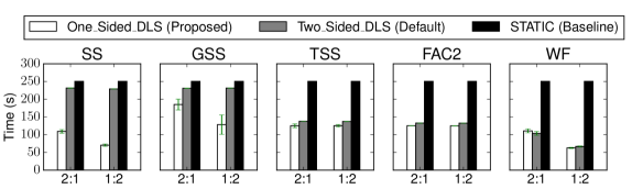
(a) The coordinator$|$master is mapped to a KNL core

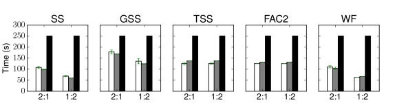
(b) The coordinator$|$master is mapped to a Xeon core

Figure 4: Performance of the proposed approach vs. the existing master-worker based approach for the PSIA. The $x$-axis represents the two ratios between the KNL cores and the Xeon cores.

Overall, Figures 4 and 5 highlight two important observations. First observation: The performance variation for executing a certain experiment using the One_Sided_DLS approach is higher than the performance variation when executing the same experiment using the Two_Sided_DLS approach. The reason behind such variation is the manner in which concurrent messages are implemented at the MPI layer in One_Sided_DLS and Two_Sided_DLS. In the current work, the Intel MPI is used to implement both approaches, One_Sided_DLS and Two_Sided_DLS. Intel MPI uses the Lock Polling strategy to implement MPI_Win_lock in which the origin process repeatedly issues lock-attempt messages to the coordinator process until the lock is granted [16]. On the contrary, Two_Sided_DLS uses the MPI_Send, MPI_Recv and MPI_Iprobe functions. For Intel MPI, in the case of simultaneous sends of multiple work requests to the master process, the master checks the outstanding work requests using MPI_Iprobe, and serves them by giving priority to the request of the process with the smallest MPI rank. The One_Sided_DLS has a high probability to grant the lock to different MPI processes at each trial, whereas, Two_Sided_DLS always prioritizes requests from the process with the smallest MPI rank. The GSS has the largest non-linear decrement among the decrements of the selected DLS techniques. Therefore, GSS is highly-sensitive to the chunk-assignment.

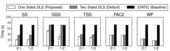
(a) The coordinator$|$master is mapped to a KNL core

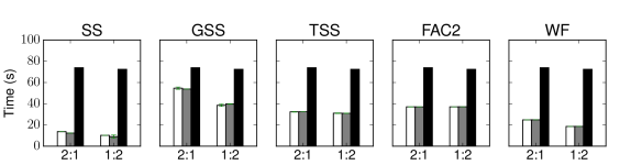
(b) The coordinator$|$master is mapped to a Xeon core

Figure 5: Performance of the proposed approach vs. the existing master-worker based approach for the Mandelbrot set. The $x$-axis represents the two ratios between the KNL cores and the Xeon cores.

Second observation: FAC and WF exhibit a reduced sensitivity to mapping the master to a KNL or to a Xeon core. This low sensitivity could be due to the factoring-based nature of these techniques. Among all the assessed DLS techniques, FAC2 and WF assign chunks in batches, which increases the possibility for the master to have chunks of the same size as the other processing elements. However, further analysis is needed to better understand such reduced sensitivity.

6 Conclusion and Future Work

A number of DLS techniques has been revisited and re-evaluated in light of and to enable them to benefit from the significant advancements in modern HPC systems, both at hardware and software levels. A distributed chunk-calculation approach (One_Sided_DLS) has been proposed herein and is implemented using the MPI RMA and atomic read-modify-write operations with passive-target synchronization mode. The One_Sided_DLS approach performs competitively against existing approaches, such as Two_Sided_DLS that uses MPI two-sided communication and employs the conventional master-worker execution model. One_Sided_DLS has the potential to alleviate the master-worker level contention of Two_Sided_DLS in large-scale HPC systems.

The present work revealed interesting aspects, planned as future work. The performance of the two approaches considered herein, One_Sided_DLS and Two_Sided_DLS, is planned to be assessed with additional applications. Specifically, the applications that require the return of the intermediate results upon the execution of each chunk of work. These applications will help to assess the impact of the data distribution on the One_Sided_DLS approach. The scalability aspect of the proposed One_Sided_DLS approach also requires further study and analysis.

References

- [1] Z. Fang, P. Tang, P.-C. Yew, and C.-Q. Zhu, “Dynamic processor self-scheduling for general parallel nested loops,” IEEE Transactions on Computers, vol. 39, no. 7, pp. 919–929, 1990.
- [2] T. Peiyi and Y. Pen-Chung, “Processor Self-Scheduling for Multiple-Nested Parallel Loops,” in Proceedings of the International Conference on Parallel Processing, August 1986, pp. 528–535.
- [3] C. D. Polychronopoulos and D. J. Kuck, “Guided Self-Scheduling: A Practical Scheduling Scheme for Parallel Supercomputers,” IEEE Transactions on Computers, vol. 100, no. 12, pp. 1425–1439, 1987.
- [4] T. H. Tzen and L. M. Ni, “Trapezoid Self-Scheduling: A Practical Scheduling Scheme for Parallel Compilers,” IEEE Transactions on parallel and distributed systems, vol. 4, no. 1, pp. 87–98, 1993.
- [5] S. Flynn Hummel, E. Schonberg, and L. E. Flynn, “Factoring: A method for scheduling parallel loops,” Communications of the ACM, vol. 35, no. 8, pp. 90–101, 1992.
- [6] S. Flynn Hummel, J. Schmidt, R. Uma, and J. Wein, “Load-sharing in heterogeneous systems via weighted factoring,” in Proceedings of the 8th annual ACM symposium on Parallel algorithms and architectures, 1996, pp. 318–328.
- [7] I. Banicescu, V. Velusamy, and J. Devaprasad, “On the scalability of dynamic scheduling scientific applications with adaptive weighted factoring,” Journal of Cluster Computing, vol. 6, no. 3, pp. 215–226, 2003.
- [8] W.-C. Shih, C.-T. Yang, and S.-S. Tseng, “A performance-based parallel loop scheduling on Grid environments,” The Journal of Supercomputing, vol. 41, no. 3, pp. 247–267, 2007.
- [9] A. T. Chronopoulos, S. Penmatsa, N. Yu, and D. Yu, “Scalable loop self-scheduling schemes for heterogeneous clusters,” International Journal of Computational Science and Engineering, vol. 1, no. 2-4, pp. 110–117, 2005.
- [10] I. Banicescu, R. L. Cariño, J. P. Pabico, and M. Balasubramaniam, “Design and implementation of a novel dynamic load balancing library for cluster computing,” Journal of Parallel Computing, vol. 31, no. 7, pp. 736–756, 2005.
- [11] R. L. Cariño and I. Banicescu, “A load balancing tool for distributed parallel loops,” Journal of Cluster Computing, vol. 8, no. 4, pp. 313–321, 2005.
- [12] C.-C. Wu, C.-T. Yang, K.-C. Lai, and P.-H. Chiu, “Designing parallel loop self-scheduling schemes using the hybrid MPI and OpenMP programming model for multi-core grid systems,” The Journal of Supercomputing, vol. 59, no. 1, pp. 42–60, 2012.
- [13] MPI Forum, “Message-Passing Interface,” https://www.mpi-forum.org, [Online; accessed 14 October 2018].
- [14] D. Bonachea and J. Duell, “Problems with using MPI 1.1 and 2.0 as compilation targets for parallel language implementations,” International Journal of High Performance Computing and Networking, vol. 1, no. 1-3, pp. 91–99, 2004.
- [15] T. Hoefler, J. Dinan, R. Thakur, B. Barrett, P. Balaji, W. Gropp, and K. Underwood, “Remote memory access programming in MPI-3,” ACM Transactions on Parallel Computing, vol. 2, no. 2, p. 9, 2015.
- [16] X. Zhao, P. Balaji, and W. Gropp, “Scalability Challenges in Current MPI One-Sided Implementations,” in International Symposium on Parallel and Distributed Computing, 2016, pp. 38–47.
- [17] H. Zhou and J. Gracia, “Asynchronous progress design for a MPI-based PGAS one-sided communication system,” in The International Conference on Parallel and Distributed Systems, 2016, pp. 999–1006.
- [18] J. R. Hammond, S. Ghosh, and B. M. Chapman, “Implementing OpenSHMEM using MPI-3 one-sided communication,” in Workshop on OpenSHMEM and Related Technologies, 2014, pp. 44–58.
- [19] H. Shan, S. Williams, Y. Zheng, W. Zhang, B. Wang, S. Ethier, and Z. Zhao, “Experiences of Applying One-sided Communication to Nearest-neighbor Communication,” in Proceedings of the First Workshop on PGAS Applications, 2016, pp. 17–24.
- [20] I. Banicescu and S. Flynn Hummel, “Balancing Processor Loads and Exploiting Data Locality in N-body Simulations,” in Proceedings of the ACM/IEEE International Conference for High Performance Computing, Networking, Storage, and Analysis, December 1995, pp. 43–43.
- [21] A. Eleliemy, A. Mohammed, and F. M. Ciorba, “Efficient Generation of Parallel Spin-images Using Dynamic Loop Scheduling,” in Proceedings of the 8th International Workshop on Multicore and Multithreaded Architectures and Algorithms of the 19th IEEE International Conference for High Performance Computing and Communications, December 2017, p. 8.
- [22] A. T. Chronopoulos, S. Penmatsa, N. Yu, and D. Yu, “Scalable Loop Self-Scheduling Schemes for Heterogeneous Clusters,” International Journal of Computational Science and Engineering, vol. 1, no. 2-4, pp. 110–117, 2005.
- [23] R. L. Cariño and I. Banicescu, “Dynamic load balancing with adaptive factoring methods in scientific applications,” The Journal of Supercomputing, vol. 44, no. 1, pp. 41–63, 2008.
- [24] A. T. Chronopoulos, R. Andonie, M. Benche, and D. Grosu, “A class of loop self-scheduling for heterogeneous clusters,” in Proceedings of International Conference on Cluster Computing, 2001, pp. 282–291.
- [25] K. Barker, A. Chernikov, N. Chrisochoides, and K. Pingali, “A load balancing framework for adaptive and asynchronous applications,” IEEE Transactions on Parallel and Distributed Systems, vol. 15, no. 2, pp. 183–192, 2004.
- [26] A. Eleliemy, “The distributed-chunk calculation approach of dynamic loop scheduling techniques ,” https://c4science.ch/source/dls_MPI_RMA/, [Online; accessed 10 December 2018].
- [27] A. Eleliemy, M. Fayze, R. Mehmood, I. Katib, and N. Aljohani, “Loadbalancing on Parallel Heterogeneous Architectures: Spin-image Algorithm on CPU and MIC,” in Proceedings of the 9th EUROSIM Congress on Modelling and Simulation, September 2016, pp. 623–628.
- [28] A. E. Johnson, “Spin-Images: A Representation for 3-D Surface Matching,” Ph.D. dissertation, Robotics Institute, Carnegie Mellon University, August 1997.
- [29] B. B. Mandelbrot, “Fractal aspects of the iteration of for complex and z,” Annals of the New York Academy of Sciences, vol. 357, no. 1, pp. 249–259, 1980.
- [30] P. Jovanovic, M. Tuba, and D. Simian, “A new visualization algorithm for the Mandelbrot set,” in Proceedings of the 10th WSEAS International Conference on Mathematics and Computers in Biology and Chemistry, 2009, pp. 162–166.
- [31] K. Wang, G. Lavoué, F. Denis, A. Baskurt, and X. He, “A benchmark for 3D mesh watermarking,” in Proceedings of the 9th IEEE International Conference on Shape Modeling and Applications, 2010, pp. 231–235.