Global and Quadratic Convergence of Newton Hard-Thresholding Pursuit

Abstract

Algorithms based on the hard thresholding principle have been well studied with sounding theoretical guarantees in the compressed sensing and more general sparsity-constrained optimization. It is widely observed in existing empirical studies that when a restricted Newton step was used (as the debiasing step), the hard-thresholding algorithms tend to meet halting conditions in a significantly low number of iterations and are very efficient. Hence, the thus obtained Newton hard-thresholding algorithms call for stronger theoretical guarantees than for their simple hard-thresholding counterparts. This paper provides a theoretical justification for the use of the restricted Newton step. We build our theory and algorithm, Newton Hard-Thresholding Pursuit (NHTP), for the sparsity-constrained optimization. Our main result shows that NHTP is quadratically convergent under the standard assumption of restricted strong convexity and smoothness. We also establish its global convergence to a stationary point under a weaker assumption. In the special case of the compressive sensing, NHTP effectively reduces to some of the existing hard-thresholding algorithms with a Newton step. Consequently, our fast convergence result justifies why those algorithms perform better than without the Newton step. The efficiency of NHTP was demonstrated on both synthetic and real data in compressed sensing and sparse logistic regression.

Keywords: sparse optimization, stationary point, Newton’s method, hard thresholding, global convergence, quadratic convergence rate

Running Title: Newton Hard-Thresholding Pursuit

1 Introduction

In this paper, we are mainly concerned with numerical methods for the sparsity constrained optimization

$$\min_{\mathbf{x}\in\mathbb{R}^{n}}\ \ f(\mathbf{x}),\qquad{\rm s.t.}\qquad\|\mathbf{x}\|_{0}\leq s,$$ (1)

where $f:\mathbb{R}^{n}\mapsto\mathbb{R}$ is continuously differentiable, $\|\mathbf{x}\|_{0}$ is the $l_{0}$ norm of $\mathbf{x}$, counting the number of nonzero elements in $\mathbf{x}$, and $s$ is a given integer regulating the sparsity level in $\mathbf{x}$ (i.e., $\mathbf{x}$ is $s$-sparse). This problem has been well investigated by Bahmani et al. (2013) (from statistical learning perspective) and Beck and Eldar (2013) (from optimization perspective). Problem (1) includes the widely studied Compressive Sensing (CS) (see, e.g., Elad (2010); Zhao (2018)) as a special case:

$$\min_{\mathbf{x}\in\mathbb{R}^{n}}\ \ f(\mathbf{x})=f_{\mbox{cs}}(\mathbf{x})=\frac{1}{2}\|A\mathbf{x}-\mathbf{b}\|^{2},\qquad{\rm s.t.}\qquad\|\mathbf{x}\|_{0}\leq s,$$ (2)

where $A$ is an $m\times n$ sensing matrix, $\mathbf{b}\in\mathbb{R}^{n}$ is the observation and $\|\cdot\|$ is the Euclidean norm in $\mathbb{R}^{n}$. Problem (1) has also been a major model in high-dimensional statistical recovery (Agarwal et al. (2010), Negahban et al. (2012)), nonlinear compressive sensing (Blumensath (2013)), and learning model-based sparsity (Bahmani et al. (2016)). An important class of algorithms makes use of the gradient information together with the hard-thresholding technique. We refer to Bahmani et al. (2013), Yuan et al. (2018) (for (1)) and Needell and Tropp (2009), Foucart (2011) (for CS) for excellent examples of such methods and their corresponding theoretical results. In terms of the numerical performance, it has been widely observed that whenever a restricted Newton step is used in the so-called debiasing step, those algorithms appear to take a significantly low number of iterations to converge, see Foucart (2011) and Remark 8 in Section 3.3. Yet, their theoretical guarantee appears no better than their pure gradient-based counterparts. Hence, there exists an intriguing gap between the exceptional empirical experience and the best convergence theory. This paper aims to provide a theoretical justification for their efficiency by establishing the quadratic convergence of such methods under standard assumptions used in the literature.

In the following, we give a selective review of past work that directly motivated our research, followed by a brief explanation of our general framework that shares a similar structure with several existing algorithms.

1.1 A selective review of past work

There exists a large number of computational algorithms that can be applied to (1). For instance, many of them can be found in Google Scholar from the many papers citing Figueiredo et al. (2007), Needell and Tropp (2009), Elad (2010) and also in the latest book by Zhao (2018). We opt to conduct a bit technical review on a small number of papers that directly motivated our research. Those reviewed papers more or less suggest the following algorithmic framework that largely obeys the principle laid out in Needell and Tropp (2009) and follow the recipes for hard-thresholding methods in Kyrillidis and Cevher (2011). Given the $k$th iterate $\mathbf{x}^{k}$, update it to the next iterate $\mathbf{x}^{k+1}$ by the following steps:

$$\left\{\begin{array}[]{ll}\mbox{Step 1 (Support Identification Process)}:&\ T_{k}=\texttt{SIP}(h(\mathbf{x}^{k})),\\[2.58334pt] \mbox{Step 2 (Debiasing)}:&\ \widetilde{\mathbf{x}}^{k+1}=\arg\min\ \left\{q_{k}(\mathbf{x}):\ \ \mathbf{x}|_{T_{k}^{c}}=0\right\},\\[2.58334pt] \mbox{Step 3 (Pruning)}:&\ \mathbf{x}^{k+1}\in{\cal P}_{s}(\widetilde{\mathbf{x}}^{k+1}).\end{array}\right.$$ (3)

We put the three steps in the perspectives of some existing algorithms and explain the notation involved. For the case of CS, the well-known CoSaMP (Compressive Sample Matching Pursuit) of Needell and Tropp (2009) chose the identification function $h(\mathbf{x})$ to be the gradient function $\nabla f(\mathbf{x})$ and the support identification process SIP is chosen to be the union of the best $2s$ support of $h(\mathbf{x}^{k})$ (i.e., the $2s$ indices that are from the $2s$ largest elements of $h(\mathbf{x}^{k})$ in magnitude) and $\mbox{supp}(\mathbf{x}^{k})$, which are the indices of nonzero elements in $\mathbf{x}^{k}$. In this case, the number of indices in $T_{k}$ is below $3s$ (i.e., $|T_{k}|\leq 3s$). In the HTP (Hard Thresholding Pursuit) algorithm of Foucart (2011), $h(\mathbf{x})$ is set to be $(\mathbf{x}-\eta\nabla f(\mathbf{x}))$, where $\eta>0$ is a step size. $T_{k}$ is chosen to be the best $s$ support of $h(\mathbf{x}^{k})$. Hence, $|T_{k}|=s$. In AIHT of Blumensath (2012) (Accelerated Iterative Hard Thresholding), $T_{k}$ is chosen as in HTP. For the general nonlinear function $f(\mathbf{x})$, the GraSP of Bahmani et al. (2013) (Gradient Support Pursuit) chose $T_{k}$ as in CoSaMP so that $T_{k}|\leq 3s$. The GraHTP of Yuan et al. (2018) (Gradient Hard Thresholding Pursuit) chose $T_{k}$ as in HTP for CS.

Once $T_{k}$ is chosen, Step 2 (debiasing step) attempts to provide a better estimate for the solution of (1) by solving an optimization problem within a restricted subspace obtained by setting all elements of $\mathbf{x}$ indexed by $T_{k}^{c}$ to zero. Here $T_{k}^{c}$ is the complementary set of $T$ in $\{1,\ldots,n\}$. Step 3 (pruning step) simply applies the hard-thresholding operator, denoted as ${\cal P}_{s}$, to $\widetilde{\mathbf{x}}^{k+1}$. To be more precise, ${\cal P}_{s}(\mathbf{x})$ contains all minimal $2$-norm distance solutions from $\mathbf{x}$ under the $s$-sparsity constraint:

$${\cal P}_{s}(\mathbf{x})={\rm argmin}_{\mathbf{z}}\left\{\|\mathbf{x}-\mathbf{z}\|\ |\ \|\mathbf{z}\|_{0}\leq s\right\},$$

which can be obtained by retaining the $s$ largest elements in magnitude from $\mathbf{x}$ and setting the remaining to zero. The great flexibility in choosing $T_{k}$ and the objective function $q_{k}(\mathbf{x})$ in the debiasing step makes it possible to derive various algorithms in literature. For instance, if we choose $T_{k}=\{1,\ldots,n\}$ (hence $T_{k}^{c}=\emptyset$) and $q_{k}(\mathbf{x})$ to be the first-order approximation of $f$ with a proximal term at $\mathbf{x}^{k}$:

$$q_{k}(\mathbf{x}):=f(\mathbf{x}^{k})+\langle\nabla f(\mathbf{x}^{k}),\ \mathbf{x}-\mathbf{x}^{k}\rangle+\frac{1}{2\eta}\|\mathbf{x}-\mathbf{x}^{k}\|^{2},$$

then we will recover the popular (gradient) hard-thresholding algorithms, see, e.g., Blumensath and Davies (2008, 2009) and Beck and Eldar (2013) for the iterated hard-thresholding algorithms, and Bahmani et al. (2013) for the restricted gradient descent and Yuan et al. (2018) for GraHTP. The CoSaMP is recovered if $T_{k}$ is chosen as in CoSaMP and $q_{k}(\mathbf{x})=f_{\mbox{cs}}(\mathbf{x})$. More existing methods can be interpreted this way and we omit the details here.

Instead, we focus on the algorithms that make use of the second order approximation in $q_{k}(\mathbf{x})$. Bahmani et al. (2013) proposed the restricted Newton step, which is equivalent to choosing $q_{k}(\mathbf{x})$ to be a restricted second-order approximation to $f(\mathbf{x})$ at $\mathbf{x}^{k}$:

$$q_{k}(\mathbf{x}):=f(\mathbf{x}^{k})+\langle\nabla f(\mathbf{x}^{k}_{T_{k}}),\ \mathbf{x}_{T_{k}}-\mathbf{x}^{k}_{T_{k}}\rangle+\frac{1}{2}\langle\mathbf{x}_{T_{k}}-\mathbf{x}^{k}_{T_{k}},\ \nabla^{2}_{T_{k}}f(\mathbf{x}^{k})(\mathbf{x}_{T_{k}}-\mathbf{x}^{k}_{T_{k}})\rangle$$ (4)

where the notation $\mathbf{x}_{T_{k}}$ denotes the restriction of $\mathbf{x}$ to the indices in $T_{k}$, $\nabla f(\mathbf{x}^{k}_{T_{k}})$ is the (partial) gradient of $f(\mathbf{x})$ with respect to the variables indexed by $T_{k}$ and evaluated at $\mathbf{x}^{k}_{T_{k}}$, and $\nabla^{2}_{T_{k}}f(\mathbf{x}^{k})$ is the principle submatrix of the Hessian matrix $\nabla^{2}f(\mathbf{x}^{k})$ indexed by $T_{k}$. In the case of CS (2), the restricted Newton step is equivalent to minimizing $q_{k}(\mathbf{x})=f_{\mbox{cs}}(\mathbf{x})$ restricted on the subspace defined by $\mathbf{x}|_{T_{k}^{c}}=0$. Hence, the restricted Newton step recovers CoSaMP. We note that in both cases, $|T_{k}|\leq 3s$ (i.e., $T_{k}$ is relatively large). In the HTP algorithm, Foucart (2011) managed to choose $T_{k}$ of size $s$ by making use of the hard thresholding technique, which is further investigated by Blumensath (2012) by the name of accelerated iterative hard-thresholding.

The benefit of using the Newton step has been particularly witnessed for the case of CS. Foucart (2011) compiled convincing numerical evidence that HTP took a significantly low number of iterations to converge when proper step-size $\eta$ is used. However, the existing theoretical guarantee for HTP is no better than their greedy counterparts (e.g., simple iterative hard-thresholding algorithms (IHT)). That is, the theory ensures that the distance between each iterate to any given reference (sparse) point is bounded by the sum of two terms. The first term converges linearly and the second term is a fixed approximation error that depends on the choice of the reference point. We refer to the latest paper of Shen and Li (2018) for many of such a result, which is often called statistical error-bound guarantee. The discrepancy between being able to offer better empirical performance than many simple IHT algorithms and only sharing similar theoretical guarantee with them invites an intriguing question: why is it so? A positive answer will inevitably provide a deep understanding of the Newton-type HTP algorithms and lead to new powerful algorithms. This is exactly what we are going to achieve in this paper.

A different line of research for (1) was initiated by Beck and Eldar (2013) from an optimization perspective. The convergence results established were drastically contrasting to the statistical error bound result mentioned above. It is proved that any accumulation point of the generated sequence by the IHT method is one kind of stationary point (i.e., $\eta$-stationarity, to be defined later). In the particular case of CS, the whole sequence converges to an $\eta$-stationary point under the $s$-regularity assumption of the sensing matrix $A$ ( i.e., any $s$ columns of $A$ are linearly independent). It is known that $2s$-regularity is a minimal condition that any two $s$-sparse vectors can be distinguished and it is often assumed by many quantities related to the restricted isometry property (RIP) of Candés and Tao (2005). The fact that the $s$-regularity is weaker than the $2s$-regularity means that many hard-thresholding algorithms actually converge to an $\eta$ stationary point of (1). Hence, the quality of those algorithms can be measured not only by their statistical error bounds, but also by the quality of the $\eta$ stationary point (e.g., whether a stationary point is optimal). We refer to Beck and Eldar (2013); Beck and Hallak (2015) for more discussion on the $\eta$ stationarity in relation to the global optimality.

Similar convergence results to Beck and Eldar (2013) have also been established in the literature of CS. Blumensath and Davies (2010) showed that the normalized IHT with an adaptive step-size rule converges to a local minimum of (2) provided that the $s$-regularity holds. This leads us to ask the following question: when the Newton step is used in a framework of IHT (such as HTP algorithm of Foucart (2011)), we would like to know whether the resulting algorithm enjoys the following fast quadratic convergence:

$$\mathbf{x}^{k}\ \ \rightarrow\ \ \mathbf{x}^{*}\qquad\mbox{and}\qquad\|\mathbf{x}^{k+1}-\mathbf{x}^{*}\|\leq c\|\mathbf{x}^{k}-\mathbf{x}^{*}\|^{2}\quad\mbox{for sufficiently large}\ k,$$ (5)

where $c$ is a constant solely dependent on the objective function $f$ (independent of the iterates $\mathbf{x}^{k}$ and its limit $\mathbf{x}^{*}$). This fast convergence result would justify the stronger numerical performance of various Newton-type methods reviewed in the first part of the subsection. Although, it is expected in optimization that Newton’s method (Nocedal and Wright (1999)) will usually lead to quadratic convergence, the problem (1) is not a standard optimization problem and it has a combinatorial nature. Hence, quadratic convergence does not follow from any existing theory from optimization. We also note that both Bahmani et al. (2013) and Yuan et al. (2018) listed the restricted Newton step as a possible variant for the debiasing step, but it was not theoretically investigated.

We finish this brief review by noticing that there are researches that exclusively studied the role of Newton’s method for (1) (see, e.g., Dai and Milenkovic (2009), Yuan and Liu (2017), Chen and Gu (2017)). However, as before, they did not offer any better theoretical guarantees than their simple greedy counterparts. Furthermore, their algorithms do not follow the general framework of (3) and hence their results cannot be used to explain the efficiency of Newton’s method that follows (3). In this paper, we will design an algorithm, that also makes uses of a restricted Newton step in the debiasing step (Step 2) and analyse its role in convergence. We will show that our algorithm enjoys the quadratic convergence (5) as well as others. We will particularly relate it to HTP of Foucart (2011) so as to justify the strong empirical performance of similar algorithms.

1.2 Our approach and main contributions

The first departure of our proposed Newton step from the one of Bahmani et al. (2013) is that we employ a different quadratic function, denoted as $q_{k}^{N}(\mathbf{x})$:

$$q_{k}^{N}(\mathbf{x}) := \mbox{the second-order Taylor expansion of $f(\mathbf{x})$ at $\mathbf{x}^{k}$, then set}\ \mathbf{x}|_{T_{k}^{c}}=0$$

$$= \langle\nabla_{T_{k}}f(\mathbf{x}^{k}),\ \mathbf{x}_{T_{k}}-\mathbf{x}^{k}_{T_{k}}\rangle+\frac{1}{2}\langle\mathbf{x}_{T_{k}}-\mathbf{x}^{k}_{T_{k}},\ \nabla^{2}_{T_{k}}f(\mathbf{x}^{k})(\mathbf{x}_{T_{k}}-\mathbf{x}^{k}_{T_{k}})\rangle$$

$$-\ \langle\mathbf{x}_{T_{k}},\ \nabla^{2}_{T_{k},T_{k}^{c}}f(\mathbf{x}^{k})(\mathbf{x}^{k}_{T_{k}^{c}})\rangle+\ (\mbox{constant term independent of $\mathbf{x}$}),$$

where $\nabla_{T_{k}}f(\mathbf{x}^{k}):=(\nabla f(\mathbf{x}^{k}))_{T_{k}}$ and $\nabla^{2}_{T_{k},T_{k}^{c}}f(\mathbf{x}^{k})$ is the submatrix whose rows and columns are from the Hessian matrix $\nabla^{2}f(\mathbf{x}^{k})$ indexed by $T_{k}$ and $T_{k}^{c}$ respectively. For the case of CS problem (2), it is straightforward to verify that $q_{k}^{N}(\mathbf{x})=q_{k}(\mathbf{x})$ in (4). Therefore, the Newton step will become the one used in CoSaMP or HTP depending on how $T_{k}$ is selected. In this paper, we choose $T_{k}$ to be the best $s$ support of $\mathbf{x}^{k}-\eta\nabla f(\mathbf{x}^{k})$. That is, $T_{k}$ contains a set of indices that define the $s$ largest absolute values in $\mathbf{x}^{k}-\eta\nabla f(\mathbf{x}^{k})$ with $\eta$ being steplength. For the case of CS, it is the same as that in the algorithm $\texttt{HTP}^{\mu}$ of Foucart (2011). For the general nonlinear function $f$, however, $q_{k}^{N}(\mathbf{x})$ and $q_{k}(\mathbf{x})$ are different. The function $q_{k}(\mathbf{x})$ in (4) is obtained in such a way that we first restrict $f(\mathbf{x})$ to the subspace $\mathbf{x}|_{T_{k}^{c}}=0$ and then approximate it by the second-order Taylor expansion (i.e., restriction and approximation). In contrast, the function $q_{k}^{N}(\mathbf{x})$ is obtained in the opposite way. We first approximate $f(\mathbf{x})$ by its second-order Taylor expansion and then restrict the approximation to the subspace $\mathbf{x}_{T_{k}^{c}}=0$ (i.e., approximation and restriction). We will see that our way of construction will allow us quantitatively bound the error $\|\mathbf{x}^{k+1}-\mathbf{x}^{*}\|$ in terms of $\|\mathbf{x}^{k}-\mathbf{x}^{*}\|$, eventually leading to the quadratic convergence in (5).

Our second innovation is to cast the Newton step as a Newton iteration for a nonlinear equation:

$$F_{\eta}(\mathbf{x},\ T_{k})=0,$$ (7)

where $F_{\eta}(\cdot,T_{k}):\mathbb{R}^{n}\mapsto\mathbb{R}^{n}$ is a function reformulated from the $\eta$ stationarity condition. We defer its technical definition to the next section. A crucial point we would like to make is that this new interpretation of the Newton step offers a fresh angle to examine it and will allow us to develop new analytical tools mainly from optimization perspective and eventually establish the promised quadratic convergence.

It is known that Newton’s method is a local method. A commonly used technique for globalization is the line search strategy, which is adopted in this paper. Therefore, we will have a Newton iterate with varying step-size. This agrees with the empirical observation that adaptive step-size in HTP often works more efficiently than other variants. Putting together the three techniques (quadratic approximation $q_{k}^{N}(\mathbf{x})$, nonlinear equation (7), and the line search strategy) will result in our proposed algorithm termed as Newton Hard-Thresholding Pursuit (NHTP) due to the Newton-step and the way how $T_{k}$ is selected being the two major components of the algorithm. We finish this section by summarizing our major contributions.

• We develop the new algorithm NHTP, which largely follows the general framework of (3) with Step 3 (pruning) to be replaced by a globalization step. The new step is achieved through the Armijo line search. We will establish its global convergence to an $\eta$ stationary point under the restricted strong smoothness of $f$.

• If $f$ is further assumed to be restricted strongly convex at the one of the accumulation points of NHTP, the Armijo line search steplength will eventually becomes $1$. Consequently, NHTP will become the restricted Newton method and leads to its convergence at a quadratic rate. This result successfully extends the classical quadratic convergence result of Newton’s method to the sparse case. For the case of CS, NHTP reduces to some known algorithms including the HTP family of Foucart (2011), with properly chosen step-sizes. The quadratic convergence result resolves the discrepancy between the strong numerical performance of HTP (and its alike) and its existing linear convergence guarantee.

• Rigorously establishing the quadratic convergence of NHTP is a major contribution of the paper. As far as we know, it is the first paper that establishes both the global and the quadratic convergence for an algorithm that employs both the Newton step and the gradient step (through the hard thresholding operator) for (1). The developed framework of analysis is innovative and will open possibility to prove that other Newton-type HTP methods may also enjoy the quadratic convergence. In our final contribution of this paper, we show experimental results in CS and the logistic regression, with both synthetic and real data, to illustrate the way NHTP works.

1.3 Organization

In the next section, we will describe the basic assumptions on the objective function $f$ and their implications. We will also develop a theoretical foundation for the Newton method to be used in a way that it also solves a system of nonlinear equations. Section 3 includes the detailed description of NHTP and its global and quadratic convergence analysis. We will particularly discuss its implication to the CS problem and compare with the methods of HTP family Foucart (2011). Since some of the proofs are quite technical, we move all of the proofs to the appendices in order to avoid interrupting presentation of the main results. We report our numerical experiments in Section 4 and conclude the paper in Section 5.

2 Assumptions, Stationarity and Interpretation of Newton’s Step

2.1 Notation

For easy reference, we list some commonly used notation below.

$:=$	means “define”
$\mathbf{x}$	a column vector and hence $\mathbf{x}^{\top}$ is a row vector.
$x_{i}$	the $i$th element of a vector $\mathbf{x}$.
$x_{(i)}$	the $i$th largest absolute value among the elements of $\mathbf{x}$.
$\rm{supp}(\mathbf{x})$	the support set of $\mathbf{x}$, namely, the set of indices of nonzero elements of $\mathbf{x}$.
$T$	index set from $\{1,2,\ldots,n\}$
$|T|$	the number of elements in $T$ (i.e., cardinality of $T$).
$T^{c}$	the complementary set of $T$ in $\{1,2,\ldots,\}\setminus T$.
$\mathbf{x}_{T}$	the sub vector of $\mathbf{x}$ containing elements indexed on $T$.
$\nabla_{T}f(\mathbf{x})$	$=(\nabla f(\mathbf{x}))_{T}$.
$\nabla^{2}f(\mathbf{x})$	the Hessian matrix of function $f(\cdot)$ at $\mathbf{x}$.
$\nabla^{2}_{T,J}f(\mathbf{x})$	the submatrix of the Hessian matrix whose rows and columns
	are respectively indexed by $T$ and $J$.
$\nabla^{2}_{T}f(\mathbf{x})$	$=\nabla^{2}_{T,T}f(\mathbf{x})$.
$\nabla^{2}_{T:}f(\mathbf{x})$	the submatrix of the Hessian matrix containing rows indexed by $T$.
$\langle\mathbf{x},\mathbf{y}\rangle$	the standard inner product for $\mathbf{x},\mathbf{y}\in\Re^{n}$.
$\|\mathbf{x}\|$	the norm induced by the standard inner product (i.e., Euclidean norm).
$\|\mathbf{x}\|_{\infty}$	$=\max\{|x_{i}|\}$ (the infinity norm of $\mathbf{x}\in\Re^{n}$).
$\|A\|_{2}$	the spectral norm of the matrix $A$.
$\|A\|$	may refer to any norm of $A$ equivalent to $\|A\|_{2}$.

${\cal P}_{s}(\mathbf{x})$ has been defined in Section 1.1. It is important to note that ${\cal P}_{s}(\mathbf{x})$ may have multiple best $s$-sparse approximations. For example, for $\mathbf{x}^{\top}=(1,2,-1,0)$ and $s=2$, ${\cal P}_{s}(\mathbf{x})$ contains two best $s$-sparse approximations: $(1,2,0,0)$ and $(0,2,-1,0)$.

2.2 Basic assumptions and stationarity

In order to study the convergence of various algorithms for the problem (1), some kind of regularities needs to be assumed. They are more or less analogous to the RIP for CS (see Candés and Tao (2005)). Those regularities often share the property of strong restricted convexity/smoothness, see Agarwal et al. (2010), Shalev-Shwartz et al. (2010), Jalali et al. (2011), Negahban et al. (2012), Bahmani et al. (2013), Blumensath (2013), and Yuan et al. (2018). We state the assumptions below in a way that is conducive to our technical proofs.

Definition 1

(Restricted strongly convex and smooth functions) Suppose that $f:\mathbb{R}^{n}\mapsto\mathbb{R}$ is a twice continuously differentiable function whose Hessian is denoted by $\nabla^{2}f(\cdot)$. Define

$$M_{2s}(\mathbf{x}):=\sup_{\mathbf{y}\in\mathbb{R}^{n}}\left\{\langle\mathbf{y},\;\nabla^{2}f(\mathbf{x})\mathbf{y}\rangle\ \bigg{|}\ |\rm{supp}(\mathbf{x})\cup\rm{supp}(\mathbf{y})|\leq 2s,\ \|\mathbf{y}\|=1\right\}$$

and

$$m_{2s}(\mathbf{x}):=\inf_{\mathbf{y}\in\mathbb{R}^{n}}\left\{\langle\mathbf{y},\;\nabla^{2}f(\mathbf{x})\mathbf{y}\rangle\ \bigg{|}\ |\rm{supp}(\mathbf{x})\cup\rm{supp}(\mathbf{y})|\leq 2s,\ \|\mathbf{y}\|=1\right\}$$

for all $s$-sparse vectors $\mathbf{x}$.

• We say $f$ is restricted strongly smooth (RSS) if there exists a constant $M_{2s}>0$ such that $M_{2s}(\mathbf{x})\leq M_{2s}$ for all $s$-sparse vectors $\mathbf{x}$. In this case, we say $f$ is $M_{2s}$-RSS. $f$ is said to be locally RSS at $\mathbf{x}$ if $M_{2s}(\mathbf{z})\leq M_{2s}$ only holds for those $s$-sparse vectors $\mathbf{z}$ in a neighborhood of $\mathbf{x}$.

• We say $f$ is restricted strongly convex (RSC) if there exists a constant $m_{2s}>0$ such that $m_{2s}(\mathbf{x})\geq m_{2s}$ for all $s$-sparse vectors $\mathbf{x}$. In this case, we say $f$ is $m_{2s}$-RSC. $f$ is said to be locally RSC at $\mathbf{x}$ if $m_{2s}(\mathbf{z})\geq m_{2s}$ only holds for those $s$-sparse vectors $\mathbf{z}$ in a neighborhood of $\mathbf{x}$.

• We say that $f$ is locally restricted Hessian Lipschitz continuous at an $s$-sparse vector $\mathbf{x}$ if there exists a Lipschitz constant $L_{f}$ and a neighborhood ${\cal N}_{s}(\mathbf{x}):=\{\mathbf{z}\in\mathbb{R}^{n}:\rm{supp}(\mathbf{x})\subseteq\rm{supp}(\mathbf{z}),\|\mathbf{z}\|_{0}\leq s\}$ such that

  $$\|\nabla^{2}_{T:}f(\mathbf{y})-\nabla^{2}_{T:}f(\mathbf{z})\|\leq L_{f}\|\mathbf{y}-\mathbf{z}\|,\ \ \ \ \forall~{}\mathbf{y},\mathbf{z}\in{\cal N}_{s}(\mathbf{x}),$$

  for any index set $T$ with $|T|\leq s$ and $T\supseteq\rm{supp}(\mathbf{x})$.

Remark 1. We note that the definition of $M_{2s}(\mathbf{x})$ and $m_{2s}(\mathbf{x})$ is taken from the definition of the restricted stable Hessian (RSH) of (Bahmani et al., 2013, Def. 1). If $m_{2s}(\mathbf{x})$ is bounded away from zero, the RSH is equivalent to the RSC and RSS putting together. Under the assumption of twice differentiability, RSS and RSC become that of Negahban et al. (2009), Shalev-Shwartz et al. (2010) and (Yuan et al., 2018, Def. 1). The local condition (iii) is a technical condition required for proving the quadratic convergence of our algorithm. Typical examples of such function satisfying (iii) include the quadratic function (2) and the quartic function studied in Beck and Eldar (2013):

$$f(\mathbf{x})=\sum_{i=1}^{\ell}\left(\mathbf{x}^{\top}A_{i}\mathbf{x}-c_{i}\right)^{2},$$

where $A_{i},i=1,\ldots,\ell$ are $n\times n$ symmetric matrices and $c_{i}$, $i=1,\ldots,\ell$ are given. By a standard calculus argument, $M_{2s}$-RSS implies

$$\left\{\begin{array}[]{l}\|\nabla f(\mathbf{x})-\nabla f(\mathbf{y})\|\leq M_{2s}\|\mathbf{x}-\mathbf{y}\|,\\[2.58334pt] f(\mathbf{x})-f(\mathbf{y})-\langle\nabla f(\mathbf{x}),\;\mathbf{x}-\mathbf{y}\rangle\leq\frac{M_{2s}}{2}\|\mathbf{x}-\mathbf{y}\|^{2},\end{array}\ \ \begin{array}[]{l}\forall\ \mathbf{x},\mathbf{y},\ |\mbox{supp}(\mathbf{x})|\leq s\\ |\mbox{supp}(\mathbf{x})\cup\mbox{supp}(\mathbf{y})|\leq 2s.\end{array}\right.$$ (8)

The properties in (8) ensure that any optimal solution of (1) must be an $\eta$-stationary point, which is a major concept introduced to the sparse optimization (1) by Beck and Eldar (2013). We state the concept below.

Definition 2

($\eta$-stationarity) (Beck and Eldar, 2013, Def. 2.3) An $s$-sparse vector $\mathbf{x}^{*}$ is called an $\eta$-stationary point of (1) if it satisfies the following relation

$$\mathbf{x}^{*}\in{\cal P}_{s}(\mathbf{x}^{*}-\eta\nabla f(\mathbf{x}^{*})).$$

Beck and Eldar (2013) called it the $L$-stationary point because $\eta$ is very much related to the Lipschitz constant $M_{2s}$ defined in (8). Lemma 2.2 in (Beck and Eldar, 2013) states that an $s$-sparse vector $\mathbf{x}^{*}$ is an $\eta$-stationary point if and only if

$$\nabla_{\Gamma}f(\mathbf{x}^{*})=0,\ \ \ \ \|\nabla_{\Gamma^{c}}f(\mathbf{x}^{*})\|_{\infty}\leq x^{*}_{(s)}/\eta.$$ (9)

where $\Gamma:=\rm{supp}(\mathbf{x}^{*})$. By invoking the proofs of (Beck and Eldar, 2013, Lemma 2.4 and Thm. 2.2) under the condition of (8), the existence of $\eta$-stationary point is ensured.

Theorem 3

(Existence of $\eta$-stationary point) (Beck and Eldar, 2013, Thm. 2.2). Suppose that there exists a constant $M_{2s}>0$ such that (8) holds. Let $\eta<1/M_{2s}$ and $\mathbf{x}^{*}$ be an optimal solution of (1). Then

• $\mathbf{x}^{*}$ is an $\eta$-stationary point;

• ${\cal P}_{s}(\mathbf{x}^{*}-\eta\nabla f(\mathbf{x}^{*}))$ contains exactly one element.

Consequently, we have

$$\mathbf{x}^{*}={\cal P}_{s}(\mathbf{x}^{*}-\eta\nabla f(\mathbf{x}^{*})).$$ (10)

We would like to make a few remarks on the significance of Thm. 3.

Remark 2. The characterization of the optimal solution $\mathbf{x}^{*}$ as a solution of the fixed-point equation (10) immediately suggests a simple iterative procedure:

$$\mathbf{x}^{k+1}\in{\cal P}_{s}(\mathbf{x}^{k}-\eta\nabla f(\mathbf{x}^{k})),\ \ \ k=0,1,2,\ldots.$$

Indeed, for the special case of CS, we have $\nabla^{2}f(\mathbf{x})=A^{\top}A$ and the fact about the relationship between the spectral norm $\|A\|_{2}$ and the quantity $M_{2s}$:

$$\|A\|_{2}^{2}=\sup_{\mathbf{y}\in\mathbb{R}^{n},\|\mathbf{y}\|=1}\langle\mathbf{y},A^{\top}A\mathbf{y}\rangle\geq\sup_{\|\mathbf{y}\|_{0}\leq 2s,\|\mathbf{y}\|=1}\langle\mathbf{y},A^{\top}A\mathbf{y}\rangle=M_{2s}.$$

When $\|A\|_{2}<1$, the unit length choice of $\eta=1$, which satisfies $1<1/\|A\|_{2}^{2}\leq 1/M_{2s}$, recovers the IHT of Blumensath and Davies (2008). Moreover, any stationary point of $\{\mathbf{x}^{k}\}$ is an $\eta$-stationary point and satisfies the fixed-point equation (10). For the case $\|A\|_{2}\geq 1$, the same conclusion holds as long as $\eta<1/M_{2s}$, see (Beck and Eldar, 2013, Remark 3.2).

Remark 3. The fixed-point equation characterization also measures how far an $s$-sparse point $\mathbf{x}$ is from being an $\eta$-stationary point (and hence a possible candidate for an optimal solution of (1)) by computing

$$h(\mathbf{x},\eta):=\mbox{dist}(\mathbf{x},\;{\cal P}_{s}(\mathbf{x}-\eta\nabla f(\mathbf{x}))),$$ (11)

which defines the shortest Euclidean distance from $\mathbf{x}$ to the set ${\cal P}_{s}(\mathbf{x}-\eta\nabla f(\mathbf{x}))$. If $h(\mathbf{x},\eta)$ is below a certain tolerance level (e.g., small enough), we may stop at $\mathbf{x}$. This halting criterion is different from those commonly used in CS literature such as in CoSaMP, GraSP, and HTP.

Our next remark is about a differentiable nonlinear equation reformulation of the fixed-point equation (10) and it will give rise to a nice interpretation of the Newton step obtained from minimizing $q_{k}^{N}(\mathbf{x})$ in (1.2). This remark is the main content of the next subsection.

2.3 Nonlinear equations and new interpretation of Newton’s step

Given a point $\mathbf{x}\in\mathbb{R}^{n}$ and $\eta>0$, we define the collection of all index sets of best $s$-support of the vector $\mathbf{x}-\eta\nabla f(\mathbf{x})$ by

$${\cal T}(\mathbf{x};\eta):=\left\{T\subset\{1,\ldots,n\}\ \bigg{|}\ \begin{array}[]{l}|T|=s,~{}T\supseteq\rm{supp}(\mathbf{z}),\\ \exists\ \mathbf{z}\in{\cal P}_{s}(\mathbf{x}-\eta\nabla f(\mathbf{x}))\end{array}\right\}.$$ (12)

That is, each $T$ in ${\cal T}(\mathbf{x};\eta)$ includes $s$ indices that define the locations of the $s$ largest absolute values among the elements of $\mathbf{x}-\eta\nabla f(\mathbf{x})$. Then for any given $T\in{\cal T}(\mathbf{x};\eta)$, we define the corresponding nonlinear equation:

$$F_{\eta}(\mathbf{x};T):=\left[\begin{array}[]{c}\nabla_{T}f(\mathbf{x})\\ \mathbf{x}_{T^{c}}\\ \end{array}\right]=0.$$ (15)

One advantage of defining the function $F_{\eta}(\mathbf{x};T)$ is that it is continuously differentiable with respect to $\mathbf{x}$ once $T$ is selected. Moreover, we have the following characterization of the fixed-point equation (10) in terms of $F_{\eta}$.

Lemma 4

Suppose $\eta>0$ is given. A point $\mathbf{x}\in\mathbb{R}^{n}$ is an $\eta$-stationary point if and only if

$$F_{\eta}(\mathbf{x};T)=0,\qquad\exists\ T\in{\cal T}(\mathbf{x};\eta).$$

Furthermore, a point $\mathbf{x}\in\mathbb{R}^{n}$ satisfies the fixed point equation (10) if and only if

$$F_{\eta}(\mathbf{x};T)=0,\qquad\forall\ T\in{\cal T}(\mathbf{x};\eta).$$

Remark 4 (Deriving a new stopping criterion) This result is instrumental and crucial to our algorithmic design. Bearing in mind that it is impossible to solve all the nonlinear equations associated with all possible $T\in{\cal T}(\mathbf{x};\eta)$ to get a solution that satisfies the fixed point equation, our hope is that solving one such equation would lead to our desired results. To monitor how accurately the equation (15) is solved, we develop a new stopping criterion that involves the gradient of $f$ in both parts indexed by $T$ and $T^{c}$.

• We note that $\mathbf{x}_{T^{c}}=0$ in (15) is easily satisfied. Hence, the magnitude $\|F_{\eta}(\mathbf{x};T)\|$ of the residual actually measures the gradient of $f$ on the $T$ part.

• Now suppose $\mathbf{x}$ satisfies (15). If follows from the definition of $T$ that

  $$|x_{j}|=|x_{j}-\eta\nabla_{j}f(\mathbf{x})|\geq|x_{i}-\eta\nabla_{i}f(\mathbf{x})|=\eta|\nabla_{i}f(\mathbf{x})|,\qquad\forall\ j\in T\ \ \mbox{and}\ \ \forall\ i\in T^{c}.$$

  This, together with $\mathbf{x}_{T^{c}}=0$ and $|T|=s$, leads to

  $$x_{(s)}=\min_{j\in T}|x_{j}|\geq\eta|\nabla_{i}f(\mathbf{x})|$$

  or equivalently

  $$|\nabla_{i}f(\mathbf{x})|\leq\frac{1}{\eta}x_{(s)},\qquad\forall\ i\in T^{c}$$ (16)

  This is the gradient condition on the $T^{c}$ part that an $\eta$-stationary point has to satisfy. Therefore, a measure on the violation of this condition indicates how close it is approximated on the $T^{c}$ part.

Consequently, a natural tolerance function to measure how far $\mathbf{x}$ is from being an $\eta$-stationary point is

$$\mbox{Tol}_{\eta}(\mathbf{x};\;T):=\|F_{\eta}(\mathbf{x};T)\|+\max_{i\in T^{c}}\left\{\max\Big{(}|\nabla_{i}f(\mathbf{x})|-x_{(s)}/\eta,\ 0\Big{)}\right\}.$$ (17)

It is easy to see that the halting function $h(\mathbf{x},\eta)=0$ in (11) implies that there exists $T\in{\cal T}(\mathbf{x};\eta)$ such that $\mbox{Tol}(\mathbf{x};\;T)=0$ and vice versa. Our purpose is to quickly find this correct $T$.

We now turn our attention to the solution methods for (15). Suppose $\mathbf{x}^{k}$ is the current approximation to a solution of (15) and $T_{k}$ is chosen from ${\cal T}(\mathbf{x}^{k};\eta)$. Then Newton’s method for the nonlinear equation (7) takes the following form to get the next iterate $\widetilde{\mathbf{x}}^{k+1}$:

$$F^{\prime}_{\eta}(\mathbf{x}^{k};T_{k})(\widetilde{\mathbf{x}}^{k+1}-\mathbf{x}^{k})=-F_{\eta}(\mathbf{x}^{k};T),$$ (18)

where $F^{\prime}_{\eta}(\mathbf{x}^{k};T_{k})$ is the Jacobian of $F_{\eta}(\mathbf{x};T_{k})$ at $\mathbf{x}^{k}$ and it assumes the following form:

$$F^{\prime}_{\eta}(\mathbf{x}^{k};T_{k})=\left[\begin{array}[]{cc}\nabla^{2}_{T_{k}}f(\mathbf{x}^{k})&\ \nabla^{2}_{T_{k},T_{k}^{c}}f(\mathbf{x}^{k})\\[2.58334pt] 0&I_{n-s}\end{array}\right].$$ (19)

Let $\mathbf{d}_{N}^{k}:=\widetilde{\mathbf{x}}^{k+1}-\mathbf{x}^{k}$ be the Newton direction. Substituting (19) into (18) yields

$$\left\{\begin{array}[]{rcl}\nabla_{T_{k}}^{2}f(\mathbf{x}^{k})(\mathbf{d}_{N}^{k})_{T_{k}}&=&\nabla_{T_{k},T_{k}^{c}}^{2}f(\mathbf{x}^{k})\mathbf{x}^{k}_{T_{k}^{c}}-\nabla_{T_{k}}f(\mathbf{x}^{k})\\[6.45831pt] (\mathbf{d}_{N}^{k})_{T^{c}_{k}}&=&-\mathbf{x}^{k}_{{T}_{k}^{c}}.\end{array}\right.$$ (20)

At this point, it is interesting to observe that the next iterate $(\widetilde{\mathbf{x}}^{k+1}=\mathbf{x}^{k}+\mathbf{d}_{N}^{k})$ is exactly the one we would get for the restricted Newton step from minimizing the restricted quadratic function $q_{k}^{N}(\mathbf{x})$ in (1.2). It is because of this exact interpretation of the restricted Newton step that it also drives the equation (15) to be eventually satisfied. In this way, we establish the global convergence to the $\eta$-stationarity. However, there are still a number of technical hurdles to overcome. We will tackle those difficulties in the next section.

3 Newton Hard-Thresholding Pursuit and Its Convergence

In this main section, we present our Newton Hard-Thresholding Pursuit (NHTP) algorithm, which largely follows the general framework (3), but with distinctive features. We already discussed the choice of $T_{k}$ (Step 1 in (3)) and the quadratic approximation function $q_{k}^{N}$ in (1.2) (Step 2 in (3)). Since $|T_{k}|=s$ and $\widetilde{\mathbf{x}}^{k+1}$ obtained is restricted to the subspace $\mathbf{x}|_{T_{k}^{c}}=0$, hence $\mbox{supp}(\widetilde{\mathbf{x}}^{k+1})\subseteq T_{k}$ and the pruning step is not necessary. Instead, we replace it with the globalization step:

$$\mbox{Step 3' (globalization)}\quad\left\{\begin{array}[]{l}\mathbf{x}^{k+1}={\cal G}(\widetilde{\mathbf{x}}^{k+1})\ \mbox{such that}\\[2.58334pt] \mbox{supp}(\mathbf{x}^{k+1})\subseteq T_{k}\ \ \mbox{and}\ \ f(\mathbf{x}^{k+1})\leq f(\mathbf{x}^{k}),\end{array}\right.$$ (21)

where ${\cal G}$ symbolically represents a globalization process to generate $\mathbf{x}^{k+1}$. We emphasize that globalization here refers to a process that will generate a sequence of iterates from any initial point and the sequence converges to an $\eta$-stationary point. The descent condition in (21) will be realized by the Armijo line search strategy (see Nocedal and Wright (1999)). We also emphasize, however, that there are other strategies that may work for globalization.

The rest of the section is to consolidate those three steps. We first examine how good is the restricted Newton direction (20) as well as the restricted gradient direction. We note that both directions were proposed in Bahmani et al. (2013). But as far as we know, they are not theoretically studied. We then describe our NHTP algorithm and present its global and quadratic convergence under the restricted strong convexity and smoothness.

3.1 Descent properties of the restricted Newton and gradient directions

Our first task is to answer whether the restricted Newton direction $\mathbf{d}_{N}^{k}$ from (20) provides a “good” descent direction for $f(\mathbf{x})$ on the restricted subspace $\mathbf{x}|_{T_{k}^{c}}=0$. We have the following result.

Lemma 5

(Descent inequality of the Newton direction) Suppose $f(\mathbf{x})$ is $m_{2s}$-restricted strongly convex and $M_{2s}$-restricted strongly smooth. Given a constant $\gamma\leq m_{2s}$ and the step-size $\eta\leq 1/(4M_{2s})$, we then have

$$\left\langle\nabla_{T_{k}}f(\mathbf{x}^{k}),\ (\mathbf{d}^{k}_{N})_{T_{k}}\right\rangle\leq-\gamma\|\mathbf{d}^{k}_{N}\|^{2}+\frac{1}{4\eta}\|\mathbf{x}^{k}_{T_{k}^{c}}\|^{2}.$$ (22)

We note that $T_{k}$ will eventually identify the true support and $\mathbf{x}^{k}_{T_{k}^{c}}$ should be close to zero when this happens. Hence, the positive term $\|\mathbf{x}^{k}_{T_{k}^{c}}\|^{2}/(4\eta)$ is eventually negligible and the restricted Newton direction is able to provide a reasonably good descent direction on the subspace $\mathbf{x}_{T_{k}^{c}}=0$. But in general (e.g., $f(\mathbf{x})$ is not restricted strongly convex), the inequality (22) may not hold and hence $\mathbf{d}^{k}_{N}$ may not provide a good descent direction at all. In this case, we opt for the restricted gradient direction (denoted by $\mathbf{d}^{k}_{g}$ to distinguish it from $\mathbf{d}^{k}_{N}$):

$$\mathbf{d}_{g}^{k}:=\left[\begin{array}[]{c}(\mathbf{d}^{k}_{g})_{T_{k}}\\[4.30554pt] (\mathbf{d}^{k}_{g})_{T_{k}^{c}}\end{array}\right]=\left[\begin{array}[]{c}-\nabla_{T_{k}}f(\mathbf{x}^{k})\\[2.58334pt] -\mathbf{x}_{T_{k}^{c}}\end{array}\right].$$ (23)

This strategy of switching to the gradient direction whenever the Newton direction is not good enough (by certain measure) appears very popular and practical in optimization, see, e.g., Nocedal and Wright (1999); Sun et al. (2002); Qi et al. (2003); Qi and Sun (2006); Zhao et al. (2010). Therefore, our search direction $\mathbf{d}^{k}$ for the globalization step (Step 3’ (21)) is defined as follows:

$$\mathbf{d}^{k}:=\left\{\begin{array}[]{ll}\mathbf{d}^{k}_{N},&\mbox{if the condition (\ref{Descent-Inequality-Newton}) is satisfied}\\[2.58334pt] \mathbf{d}_{g}^{k},&\mbox{otherwise}.\end{array}\right.$$ (24)

It is important to note that the choice of $\gamma$ and $\eta$ in Lemma 5 is sufficient but not necessary for the Newton direction to be used. The inequality (22) may also hold if $\gamma$ and $\eta$ violate the required bounds. This has been experienced in our numerical experiments.

Our next result further shows that the search direction $\mathbf{d}^{k}$ is actually a descent direction for $f(\mathbf{x})$ at $\mathbf{x}^{k}$ with respect to the full space $\mathbb{R}^{n}$ provided that $\eta$ is properly chosen. Suppose we have three constants $\gamma$, $\sigma$ and $\beta$ such that

$$0<\gamma\leq\min\{1,\;2M_{2s}\},\ \ 0<\sigma<1/2,\ \ \mbox{and}\ \ 0<\beta<1.$$ (25)

They will be used in our NHTP algorithm. We note that this choice implies $M_{2s}/\gamma>\sigma$. Define two more constants based on them:

$$\overline{\alpha}:=\min\left\{\frac{1-2\sigma}{M_{2s}/\gamma-\sigma},\ 1\right\}\ \ \ \mbox{and}\ \ \ \overline{\eta}:=\min\left\{\frac{\gamma(\overline{\alpha}\beta)}{M_{2s}^{2}},\ \overline{\alpha}\beta,\ \frac{1}{4M_{2s}}\right\}.$$ (26)

Lemma 6

(Descent property of $\mathbf{d}^{k}$) Suppose $f(\mathbf{x})$ is $M_{2s}$-restricted strongly smooth. Let $\gamma,\sigma$ and $\beta$ be chosen as in (25). Suppose $\eta<\overline{\eta}$ and $\mbox{supp}(\mathbf{x}^{k})\subseteq T_{k-1}$ (this will be automatically ensured by our algorithm). We then have

$$\langle\nabla f(\mathbf{x}^{k}),\;\mathbf{d}^{k}\rangle\leq-\rho\|\mathbf{d}^{k}\|^{2}-\frac{\eta}{2}\|\nabla_{T_{k-1}}f(\mathbf{x}^{k})\|^{2},$$ (27)

where $\rho>0$ is given by

$$\rho:=\min\left\{\frac{2\gamma-\eta M^{2}_{2s}}{2},\ \frac{2-\eta}{2}\right\}.$$

Lemma 6 will ensure that our algorithm NHTP is well defined.

3.2 NHTP and its convergence

Having settled that $\mathbf{d}^{k}$ is a descent direction of $f(\mathbf{x})$ at $\mathbf{x}^{k}$, we compute the next iterate along the direction $\mathbf{d}^{k}$ but restricted to the subspace $\mathbf{x}|_{T_{k}}=0$: $\mathbf{x}^{k+1}=\mathbf{x}^{k}(\alpha_{k})$ with $\alpha_{k}$ being calculated through the Armijo line search and

$$\mathbf{x}^{k}(\alpha):=\left[\begin{array}[]{c}\mathbf{x}^{k}_{T_{k}}+\alpha\mathbf{d}^{k}_{T_{k}}\\[2.58334pt] \mathbf{x}^{k}_{T_{k}^{c}}+\mathbf{d}^{k}_{T_{k}^{c}}\end{array}\right]=\left[\begin{array}[]{c}\mathbf{x}^{k}_{T_{k}}+\alpha\mathbf{d}^{k}_{T_{k}}\\[2.58334pt] 0\end{array}\right],\qquad\alpha>0.$$ (28)

Our algorithm is described in Table 1.

Table 1: Framework of NHTP

NHTP: Newton Hard-Thresholding Pursuit
Step 0	Initialize $\mathbf{x}^{0}$. Choose $\eta,\gamma>0,\sigma\in(0,1/2),\beta\in(0,1)$. Set $k\Leftarrow 0$.
Step 1	Choose $T_{k}\in{\cal T}(\mathbf{x}^{k};\eta)$.
Step 2	If ${\tt Tol}_{\eta}(\mathbf{x}^{k};T_{k})=0$, then stop. Otherwise, go to Step 3.
Step 3	Compute the search direction $\mathbf{d}^{k}$ by (24).
Step 4	Find the smallest integer $\ell=0,1,\ldots$ such that
	$$f(\mathbf{x}^{k}(\beta^{\ell}))\leq f(\mathbf{x}^{k})+\sigma\beta^{\ell}\langle\nabla f(\mathbf{x}^{k}),\mathbf{d}^{k}\rangle.$$ (29)
	Set $\alpha_{k}=\beta^{\ell}$, $\mathbf{x}^{k+1}=\mathbf{x}^{k}(\alpha_{k})$ and $k\Leftarrow k+1$, go to Step 1.

Remark 5. We will see that NHTP has a fast computational performance because of two factors. One is that it terminates in a low number of iterations due to the quadratic convergence (to be proved) and this has been experienced in our numerical experiments. The other is the low computational complexity of each step. For example, for both CS and sparse logistic regression problems, the computational complexity of each step is $\mathcal{O}(s^{3}+ms^{2}+mn+ms\ell)$, where $\ell$ is the smallest integer satisfying (29) and it often assumes the value $1$. The way $\mathbf{x}^{k}(\alpha)$ is defined guarantees that $\mbox{supp}(\mathbf{x}^{k+1})\subseteq T_{k}$ for all $k=0,1,\ldots,$. If ${\tt Tol}_{\eta}(\mathbf{x}^{k};T_{k})=0$, then $\mathbf{x}^{k}$ is already an $\eta$-stationary point and we should terminate the algorithm. Without loss of any generality, we assume that NHTP generates an infinite sequence $\{\mathbf{x}^{k}\}$ and we will analyse its convergence properties. The line search condition (29) is known as the Armijo line search and ensures a sufficient decrease from $f(\mathbf{x}^{k})$ to $f(\mathbf{x}^{k+1})$. Therefore, the two properties in the globalization step (21) is guaranteed, provided that the line search in (29) is successful. This is the main claim of the following result.

Lemma 7

(Existence and boundedness of $\alpha_{k}$) Suppose$f(\mathbf{x})$ is $M_{2s}$-restricted strongly smooth. Let the parameters $\gamma$, $\sigma$ and $\beta$ satisfy the conditions in (25) and $\overline{\alpha}$ and $\overline{\eta}$ be defined in (26). Suppose ${\tt Tol}_{\eta}(\mathbf{x}^{k};T_{k})\not=0$. For any $\alpha$ and $\eta$ satisfying

$$0<\alpha\leq\overline{\alpha}\qquad\mbox{and}\qquad 0<\eta<\min\left\{\frac{\alpha\gamma}{M^{2}_{2s}},\ \alpha,\ \frac{1}{4M_{2s}}\right\},$$

it holds

$$f(\mathbf{x}^{k}(\alpha))\leq f(\mathbf{x}^{k})+\sigma\alpha\langle\nabla f(\mathbf{x}^{k}),\;\mathbf{d}^{k}\rangle.$$ (30)

Consequently, if we further assume that $\eta\leq\overline{\eta}$, we have

$$\alpha_{k}\geq\beta\overline{\alpha}\qquad\forall\ k=0,1,\ldots,.$$

It is worth noting that the objective function is only assumed to be restricted strongly smooth (not necessarily to be restricted strongly convex). Lemma 7 not only ensures the existence of $\alpha_{k}$ that satisfies the line search condition (29), but also guarantees that $\alpha_{k}$ is always bounded away from zero by a positive margin $\beta\overline{\alpha}$. This boundedness property will in turn ensure that NHTP will converge. Our first result on convergence is about a few quantities approaching zero.

Lemma 8

(Converging quantities) Suppose $f(\mathbf{x})$ is $M_{2s}$-restricted strongly smooth. Let the parameters $\gamma$, $\sigma$ and $\beta$ satisfy the conditions in (25) and $\overline{\eta}$ be defined in (26). We further assume that $\eta\leq\overline{\eta}$. Then the following hold.

• $\{f(\mathbf{x}^{k})\}$ is a nonincreasing sequence and if $\mathbf{x}^{k+1}\not=\mathbf{x}^{k}$, then $f(\mathbf{x}^{k+1})<f(\mathbf{x}^{k})$.

• $\|\mathbf{x}^{k+1}-\mathbf{x}^{k}\|\rightarrow 0$;

• $\|F_{\eta}(\mathbf{x}^{k};\;T_{k})\|\rightarrow 0$;

• $\|\nabla_{T_{k}}f(\mathbf{x}^{k})\|\rightarrow 0$ and $\|\nabla_{T_{k-1}}f(\mathbf{x}^{k})\|\rightarrow 0$.

Those converging quantities are the basis for our main results below. They also justify the halting conditions that we will use in our numerical experiments.

Theorem 9

(Global convergence) Suppose$f(\mathbf{x})$ is $M_{2s}$-restricted strongly smooth. Let the parameters $\gamma$, $\sigma$ and $\beta$ satisfy the conditions in (25) and $\overline{\eta}$ be defined in (26). We further assume that $\eta\leq\overline{\eta}$. Then the following hold.

• Any accumulation point, say $\mathbf{x}^{*}$, of the sequence $\{\mathbf{x}^{k}\}$ is an $\eta$-stationary point of (1). If $f$ is a convex function, then for any given reference point $\mathbf{x}$ we have

  $$f(\mathbf{x}^{*})\leq f(\mathbf{x})+\frac{x^{*}_{(s)}}{\eta}\|\mathbf{x}_{\Gamma_{*}^{c}}\|_{1},$$ (31)

  where $\Gamma_{*}:=\mbox{supp}(\mathbf{x}^{*})$.

• If $\mathbf{x}^{*}$ is isolated, then the whole sequence converges to $\mathbf{x}^{*}$. Moreover, we have the following characterization on the support of $\mathbf{x}^{*}$.

  • If $\|\mathbf{x}^{*}\|_{0}=s$, then

    $$\mbox{supp}(\mathbf{x}^{*})=\mbox{supp}(\mathbf{x}^{k})=T_{k}\quad\mbox{for all sufficiently large }k.$$

  • If $\|\mathbf{x}^{*}\|_{0}<s$, then

    $$\mbox{supp}(\mathbf{x}^{*})\subseteq\mbox{supp}(\mathbf{x}^{k})\cap T_{k}\quad\mbox{for all sufficiently large }k.$$

Remark 6. Under the assumption of $f$ being restricted strongly smooth, NHTP shares the most desirable convergence property (i.e., to $\eta$-stationary point) of the iterative hard-thresholding algorithm of Beck and Eldar (2013). If $f$ is assumed to be convex, then (31) implies that for any given $\epsilon>0$, there exists neighborhood ${\cal N}(\mathbf{x}^{*})$ of $\mathbf{x}^{*}$ such that $f(\mathbf{x}^{*})\leq f(\mathbf{x})+\epsilon$ for any $\mathbf{x}\in{\cal N}(\mathbf{x}^{*})$. In particular, if $\|\mathbf{x}^{*}\|_{0}=s$, then $\mathbf{x}^{*}$ is a local minimum of (1). If $\|\mathbf{x}^{*}\|_{0}<s$ (so that $x^{*}_{(s)}=0$), then $\mathbf{x}^{*}$ is a global optimum of (1).

It achieves more. If the generated sequence converges to $\mathbf{x}^{*}$, the support of $\mathbf{x}^{*}$ is eventually identified as $T_{k}$ provided that the sparse level of $\mathbf{x}^{*}$ is $s$. If $\|\mathbf{x}^{*}\|_{0}<s$, its support would be eventually included in $T_{k}$. When specialized to the CS problem (2) with $s$-regularity, the whole sequence $\{\mathbf{x}^{k}\}$ will convergence to one point $\mathbf{x}^{*}$. This is because that any $\eta$-stationary point of the CS problem under the $s$-regularity is isolated, see (Beck and Eldar, 2013, Lemma 2.1 and Corollary 2.1). Our next result implies that under the $2s$-regularity, the whole sequence $\{\mathbf{x}^{k}\}$ converges to $\mathbf{x}^{*}$ at a quadratic rate.

Theorem 10

(Quadratic convergence) Suppose all conditions as in Thm. 9 hold. Let $\mathbf{x}^{*}$ be one of the accumulation points of $\{\mathbf{x}^{k}\}$. We further assume $f(\mathbf{x})$ is $m_{2s}$-restricted strongly convex in a neighborhood of $\mathbf{x}^{*}$. If $\gamma\leq\min\{1,\ m_{2s}\}$ and $\eta\leq\overline{\eta}$, then the following hold.

• The whole sequence $\{\mathbf{x}^{k}\}$ converges to $\mathbf{x}^{*}$, which is necessarily an $\eta$-stationary point.

• The Newton direction is accepted for sufficiently large $k$.

• If we further assume that $f$ is locally restricted Hessian Lipschitz continuous at $\mathbf{x}^{*}$ with the Lipschitz constant $L_{f}$. The line search steplength eventually becomes unity and the convergence rate of $\{\mathbf{x}^{k}\}$ to $\mathbf{x}^{*}$ is quadratic. That is, there exists an iteration index $k_{0}$ such that

  $$\alpha_{k}\equiv 1,\ \ \ \ \|\mathbf{x}^{k+1}-\mathbf{x}^{*}\|\leq\frac{L_{f}}{2m_{2s}}\|\mathbf{x}^{k}-\mathbf{x}^{*}\|^{2},\qquad\forall\ k\geq k_{0}.$$ (32)

  Moreover, for sufficiently large $k$, we have

  $$\|F_{\eta}(\mathbf{x}^{k+1};\;T_{k+1})\|\leq\frac{L_{f}\sqrt{M_{2s}^{2}+1}}{\min\{m^{3}_{2s},m_{2s}\}}\|F_{\eta}(\mathbf{x}^{k};\;T_{k})\|^{2}.$$

Remark 7. Taking into account of Lemma 8(iii) that $\|F_{\eta}(\mathbf{x}^{k};\;T_{k})\|$ converges to $0$, Thm. 10(iii) asserts that it converges at a quadratic rate. Compared with the quadratic convergence (32), the quadratic convergence in $\|F_{\eta}(\mathbf{x}^{k};\;T_{k})\|$ has the advantage that it is computationally verifiable. The quantity is also a major part of our stopping criterion in monitoring $\mbox{Tol}_{\eta}(\mathbf{x}^{k};\;T_{k})$ of (17), see Sect. 4. In addition, we proved the existence of $k_{0}$. The proof of Thm. 10(iii) suggests that $k_{0}$ should be near to the iteration when the support sets of the sequence start to be identified to be the correct support set at its limit. However, deriving an explicit form of $k_{0}$ is somehow difficult and would require extra conditions.

3.3 The case of CS

We use this part to demonstrate the application and implication of our main convergence results to the CS problem (2). We will also discuss the similarities to and differences from the existing algorithms, in particular the HTP family of Foucart (2011). The purpose is to show that there is a wide range of choices for the parameters that will lead to quadratic convergence. This is best done in terms of the restricted isometry constant (RSC) of the sensing matrix $A$. We recall from Candés and Tao (2005) that RSC $\delta_{s}$ is the smallest $\delta\geq 0$ such that

$$(1-\delta)\|\mathbf{x}\|^{2}\leq\|A\mathbf{x}\|^{2}\leq(1+\delta)\|\mathbf{x}\|^{2}\qquad\forall\ \|\mathbf{x}\|_{0}\leq s.$$

We will use $\delta_{2s}$, which is assumed to be positive throughout. For this setting, we have

$$m_{2s}=1-\delta_{2s},\quad M_{2s}=1+\delta_{2s},\quad\mbox{and}\quad\mu_{2s}:=\frac{M_{2s}}{m_{2s}}>1,$$

where, $\mu_{2s}$ is known as the $2s$-restricted stable Hessian coefficient of $A$ in Bahmani et al. (2013). For simplicity, we choose a particular set of parameters used in our NHTP to illustrate our results (many other choices are also possible). Let

$$\beta=\frac{1}{4},\quad\gamma=m_{2s},\quad\sigma=\frac{1-w}{2-w/\mu_{2s}}\ \ \mbox{with}\ \ 0<w<1.$$

It is easy to see that $\sigma\in(0,1/2)$ for any choice $w$ between $0$ and $1$. This set of parameter choices certainly satisfies the condition (25). We now calculate $\overline{\alpha}$ and $\overline{\eta}$ defined in (26). The definition of $\overline{\alpha}$ chooses

$$\overline{\alpha}\overset{(\ref{alpha-eta})}{=}\frac{1-2\sigma}{M_{2s}/\gamma-\sigma}=\frac{1-2\sigma}{\mu_{2s}-\sigma}=\frac{w}{\mu_{2s}}\in(0,1).$$

Since $\gamma/M_{2s}^{2}=1/(\mu_{2s}M_{2s})<1$ and $\beta=1/4$, we have

$$\overline{\eta} \overset{(\ref{alpha-eta})}{=} \frac{\gamma}{M_{2s}^{2}}\overline{\alpha}\beta=\frac{1}{4}\times\frac{1}{\mu_{2s}}\times\frac{1}{M_{2s}}\times\overline{\alpha}$$

$$\geq \frac{1}{4}\times\frac{1}{\mu_{2s}}\times\frac{1}{2}\times\frac{w}{\mu_{2s}}\qquad(\mbox{because}\ M_{2s}\leq 2)$$

$$= \frac{w}{8\mu^{2}_{2s}}.$$

Direct application of Thm. 10 yields the following corollary.

Corollary 11

Suppose the RIC $\delta_{2s}>0$ and the parameters of NHTP are chosen as follows:

$$\beta=\frac{1}{4},\ \ {{\sigma=\frac{1-w}{2-w/\mu_{2s}}}},\ \ \gamma=m_{2s},\ \ \eta\leq\frac{w}{8\mu^{2}_{2s}}\ \ \mbox{with}\ \ 0<w<1.$$ (33)

Then NHTP is well-defined. In particular, the Newton direction $d^{k}_{N}$ is always accepted as the search direction in (24) at each iteration. Moreover, NHTP enjoys all the three convergence results in Thm. 10.

Remark 8. (On RIC conditions) In the literature of CS, a benchmark condition (for theoretical investigation) often takes the form $\delta_{t}\leq\delta_{*}$ with $t$ being an integer. Suppose $\delta_{2s}\leq\delta_{*}$. It is easy to define and derive the following.

$$m_{2s}^{*} := 1-\delta_{*}\leq 1-\delta_{2s}=m_{2s}$$

$$\mu_{2s}^{*} := \frac{1+\delta_{*}}{1-\delta_{*}}\geq\frac{1+\delta_{2s}}{1-\delta_{2s}}=\mu_{2s}$$

$$\overline{\eta}^{*} := \frac{w}{8(\mu^{*}_{2s})^{2}}\leq\frac{w}{8\mu^{2}_{2s}}.$$

Therefore, in the selection of the parameters in (33), $\mu_{2s}$ and $m_{2s}$ can be respectively replaced by $\mu^{*}_{2s}$ and $m^{*}_{2s}$, and $\eta$ can be chosen to satisfy $\eta\leq\overline{\eta}^{*}$. In the scenario of Garg and Khandekar (2009) where $\delta_{*}=1/3$, with $w=0.5$ we could choose the parameters as $\beta=1/4$, $\gamma=2/3$, $\sigma=2/7$ and $\eta=1/64$. This set of choices would ensure NHTP converges quadratically under the RIP condition $\delta_{2s}\leq\delta_{*}=1/3$.

Remark 9. (On Newton’s direction) That the Newton direction is always accepted at each iteration is because the inequality (22) is always satisfied with the parameter selection in (33) (its proof can be patterned after that for Thm. 10(iii)). Therefore, the Newton direction $\mathbf{d}^{k}_{N}$ at each iteration takes the form:

$$\Big{(}\mathbf{d}^{k}_{N}\Big{)}_{T_{k}} = \Big{(}A^{\top}_{T_{k}}A_{T_{k}}\Big{)}^{-1}\Big{(}A_{T_{k}}^{\top}A_{T_{k}^{c}}\mathbf{x}^{k}_{T_{k}^{c}}-A_{T_{k}}^{\top}(A\mathbf{x}^{k}-\mathbf{b})\Big{)}$$

$$= \Big{(}A^{\top}_{T_{k}}A_{T_{k}}\Big{)}^{-1}\Big{(}A_{T_{k}}^{\top}A_{T_{k}^{c}}\mathbf{x}^{k}_{T_{k}^{c}}-A_{T_{k}}^{\top}(A_{T_{k}}\mathbf{x}^{k}_{T_{k}}+A_{T_{k}^{c}}\mathbf{x}^{k}_{T_{k}^{c}}-\mathbf{b})\Big{)}$$

$$= -\mathbf{x}^{k}_{T_{k}}+\Big{(}A^{\top}_{T_{k}}A_{T_{k}}\Big{)}^{-1}A_{T_{k}}^{\top}\mathbf{b}.$$

Since the unit line search steplength $\alpha_{k}=1$ is always accepted for all $k$ sufficiently large (say, $k\geq k_{0}$), we have

$$\mathbf{x}^{k+1}=\mathbf{x}^{k}(\alpha_{k})=\mathbf{x}^{k}(1)=\left[\begin{array}[]{c}\mathbf{x}^{k}_{T_{k}}+(\mathbf{d}^{k}_{N})_{T_{k}}\\ 0\end{array}\right]=\left[\begin{array}[]{c}\Big{(}A^{\top}_{T_{k}}A_{T_{k}}\Big{)}^{-1}A_{T_{k}}^{\top}\mathbf{b}\\ 0\end{array}\right]$$

Equivalently,

$$\mathbf{x}^{k+1}=\arg\min\left\{\|\mathbf{b}-A\mathbf{z}\|:\ \ \mbox{supp}(\mathbf{z})\subseteq T_{k}\right\}.$$

Consequently, NHTP eventually (when $k\geq k_{0}$) becomes $\texttt{HTP}^{\eta}$ of Foucart (2011):

$$\texttt{HTP}^{\eta}:\quad\left\{\begin{array}[]{ll}T_{k}&=\left\{\mbox{the best $s$ support of}\ (\mathbf{x}^{k}-\eta\nabla f(\mathbf{x}^{k}))\right\},\quad(\mbox{i.e.,}\ T_{k}\in{\cal T}(\mathbf{x}^{k};\eta))\\[4.30554pt] \mathbf{x}^{k+1}&=\arg\min\left\{\|\mathbf{b}-A\mathbf{z}\|:\ \ \mbox{supp}(\mathbf{z})\subseteq T_{k}\right\}.\end{array}\right.$$

(Foucart, 2011, Prop. 3.2) states that $\texttt{HTP}^{\eta}$ will converge provided that $\eta\|A\|_{2}^{2}<1$, which is ensured when $\eta<1/M_{2s}$. Our choice $\eta\leq w/(8\mu_{2s}^{2})$ apparently satisfies this condition. Hence, NHTP eventually enjoys all the good properties stated for $\texttt{HTP}^{\eta}$ under the same conditions assumed in Foucart (2011) as long as the $\eta$ (note: $\mu$ is used in Foucart (2011) instead of $\eta$) used there does not clash with our choice.

Since the Newton direction is always accepted as the search direction every iteration, one may wonder why we did not just use the unit steplength $\alpha_{k}=1$. We note that NHTP does not just seek for the next iterate satisfying $f(\mathbf{x}^{k+1})\leq f(\mathbf{x}^{k})$, it also requires it to deduce a sufficient decrease by the quantity $\alpha_{k}\sigma\langle\nabla f(\mathbf{x}^{k}),\ \mathbf{d}^{k}\rangle$, which is proportional to the steplength $\alpha_{k}$. Newton’s direction $\mathbf{d}^{k}_{N}$ with the unit steplength may not provide this proportional decrease and hence the unit steplength cannot be accepted in this case (but the unit steplength will be eventually accepted). In contrast, the HTP family algorithms of Foucart (2011) only require a decrease $f(\mathbf{x}^{k+1})\leq f(\mathbf{x}^{k})$. It is interesting to note that, in optimization, one of the guidelines in designing a descent algorithm is to ensure it deduces a sufficient decrease every iteration (see Nocedal and Wright (1999)) in order to achieve desirable convergence properties.

Remark 10. (On the gradient direction) When the information on $\mu_{2s}$ and $m_{2s}$ is difficult to estimate, the choice of (33) may not be possible. On the one hand, those are the sufficient conditions for the Newton direction to be accepted. Numerical experiments show that Newton’s direction is often accepted with a wide range of parameter choices. On the other hand, we have the restricted gradient direction to rescue if the Newton direction is not deemed to be good enough in terms of the condition (22). The resulting algorithm still enjoys the global convergence in Thm. 9 even if all search directions are of gradients. It is interesting to note that a restricted gradient method was also proposed in Foucart (2011) and is referred to as fast HTP. We describe this algorithm (with just one gradient iteration each step) in terms of our technical terminologies.

$$\texttt{FHTP}^{\eta}:\quad\left\{\begin{array}[]{ll}\widetilde{\mathbf{x}}^{k+1}&=\ {\cal P}_{s}(\mathbf{x}^{k}-\eta\nabla f(\mathbf{x}^{k}))\\ T_{k+1}&\in\ {\cal T}(\widetilde{\mathbf{x}}^{k+1};\eta)\\ \mathbf{x}^{k+1}_{T_{k+1}}&=\ \Big{(}\widetilde{\mathbf{x}}^{k+1}-t_{k+1}\nabla f(\widetilde{\mathbf{x}}^{k+1})\Big{)}_{T_{k+1}}\ \ \mbox{and}\ \ \mathbf{x}^{k+1}_{T_{k+1}^{c}}=0,\end{array}\right.$$

where $t_{k+1}$ can be set to $1$ or chosen adaptively. Despite it being also shown to enjoy similar convergence properties as $\texttt{HTP}^{\eta}$ in Foucart (2011), it does not fall within the framework (3) and (21). A noticeable difference is that $\texttt{FHTP}^{\eta}$ solves two optimization problems each step: one for $\widetilde{\mathbf{x}}^{k+1}$ and the other for $\mathbf{x}^{k+1}_{T_{k+1}}$. It would be interesting to see how the convergence analysis conducted in this paper can be extended to $\texttt{FHTP}^{\eta}$.

4 Numerical Experiments

In this part, we show experimental results of NHTP in CS (Sect. 4.1) and sparse logistic regression (Sect. 4.2) on both synthetic and real data. A general conclusion is that NHTP is capable of producing solutions of high quality and is very fast when benchmarked against six leading solvers from compressed sensing and three solvers from sparse logistic regression. All experiments were conducted by using MATLAB (R2018a) on a desktop of 8GB memory and Inter(R) Core(TM) i5-4570 3.2Ghz CPU.

We first describe how NHTP was set up. We initialize NHTP with $\mathbf{x}^{0}=0$ if $\nabla f(0)\neq 0$ and $\mathbf{x}^{0}=\textbf{1}$ if $\nabla f(0)=0$. Parameters are set as $\sigma=10^{-4}/2,\beta=0.5$. For $\gamma$, theoretically any positive $\gamma\leq m_{2s}$ is fine, but in practice to guarantee more steps using Newton directions, it is supposed to be relatively small (De Luca et al., 1996; Facchinei and Kanzow, 1997). Thus we choose $\gamma=\gamma_{k}$ with updating

$$\gamma_{k}=\left\{\begin{array}[]{ccc}10^{-10},&{\rm if}&\mathbf{x}^{k}_{T^{c}_{k}}=0,\\ 10^{-4},&{\rm if}&\mathbf{x}^{k}_{T^{c}_{k}}\neq 0.\end{array}\right.$$

For parameter $\eta$, in spite of that Theorem 10 has suggested to set $0<\eta<\overline{\eta}$, it is still difficult to fix a proper one since $M_{2s}$ is not easy to compute in general. Overall, we choose to update $\eta$ adaptively. Typically, we use the following rule: starting $\eta$ with a fixed scalar associated with the dimensions of a problem and then update it as,

$$\eta_{0} = \frac{10(1+s/n)}{\min\{10,\ln(n)\}}>1,$$

$$\eta_{k+1} = \left\{\begin{array}[]{ll}\eta_{k}/1.05,&\text{if}~{}{\rm mod}(k,10)=0~{}\text{and}\ \|F_{\eta_{k}}(\mathbf{x}^{k};T_{k})\|>k^{-2},\\ 1.05\eta_{k},&\text{if}~{}{\rm mod}(k,10)=0~{}\text{and}\ \|F_{\eta_{k}}(\mathbf{x}^{k};T_{k})\|\leq k^{-2},\\ \eta_{k},&\text{otherwise}.\end{array}\right.$$

where mod $(k,10)=0$ means $k$ is a multiple of $10$. We terminate our method if at $k$th step it meets one of the following conditions:

• $\mbox{Tol}_{\eta_{k}}(\mathbf{x}^{k};\;T_{k})\leq 10^{-6}$, where $\mbox{Tol}_{\eta}(\mathbf{x};\;T)$ is defined as (17);

• $|f(\mathbf{x}^{k+1})-f(\mathbf{x}^{k})|<10^{-6}(1+|f(\mathbf{x}^{k})|)$.

• $k$ reaches the maximum number (e.g., 2000) of iterations.

4.1 Compressed Sensing

Compressed sensing (CS) has seen revolutionary advances both in theory and algorithms over the past decade. Ground-breaking papers that pioneered the advances are (Donoho, 2006; Candés et al., 2006; Candés and Tao, 2005). The model is described as in (2)

a) Testing examples. We will focus on the exact recovery $\mathbf{b}=A\mathbf{x}$ by utilizing the sensing matrix $A$ chosen as in (Yin et al., 2015; Zhou et al., 2016).

Example 1 (Gaussian matrix)

Let $A\in\mathbb{R}^{m\times n}$ be a random Gaussian matrix with each column $A_{j},j\in N_{n}$ being identically and independently generated from the standard normal distribution. We then normalize each column such that $\|A_{j}\|=1$. Finally, the ‘ground truth’ signal $\mathbf{x}^{*}$ and the measurement $\mathbf{b}$ are produced by the following pseudo Matlab codes:

$$\mathbf{x}^{*}=\verb"zeros"(n,1),~{}~{}\Gamma=\verb"randperm"(n),~{}~{}\mathbf{x}^{*}(\Gamma(1:s))=\verb"randn"(s,1),~{}~{}\mathbf{b}=A\mathbf{x}^{*}.$$ (35)

Example 2 (Partial DCT matrix)

Let $A\in\mathbb{R}^{m\times n}$ be a random partial discrete cosine transform (DCT) matrix generated by

$$A_{ij}=\cos(2\pi(j-1)\psi_{i}),~{}~{}i=1,\ldots,m,~{}~{}j=1,\ldots,n$$

where $\psi_{i},i=1,\ldots,m$ is uniformly and independently sampled from $[0,1]$. We then normalize each column such that $\|A_{j}\|=1$ with $\mathbf{x}^{*}$ and $\mathbf{b}$ being generated the same way as in Example 1.

b) Benchmark methods. There exists a large number of numerical methods for the CS problem (2). It is beyond the scope of this paper to compare them all. We selected six state-of-the-art methods. They are HTP  (Foucart, 2011), NIHT (Blumensath and Davies, 2010), GP (Blumensath and Davies, 2008)2, OMP (Pati et al., 1993; Tropp and Gilbert, 2007)2, CoSaMP (Needell and Tropp, 2009)3 and SP (Dai and Milenkovic, 2009). For HTP, set MaxNbIter=1000 and mu=‘NHTP’. For NIHT, the maximum iteration ‘maxIter’ is set as 1000 and ${\tt M}=s$. For GP and OMP, the ‘stopTol’ is set as $1000$. For CoSaMP and SP, set tol$=10^{-6}$ and maxiteration$=1000$. Notice that the first three methods prefer solving sensing matrix $A$ with unit columns, which is the reason for us to normalize each generated $A$ in Example 1 and Example 2. Let $\mathbf{x}$ be the solution produced by a method. We say a recovery of this method is successful if $\|\mathbf{x}-\mathbf{x}^{*}\|<0.01\|\mathbf{x}^{*}\|.$

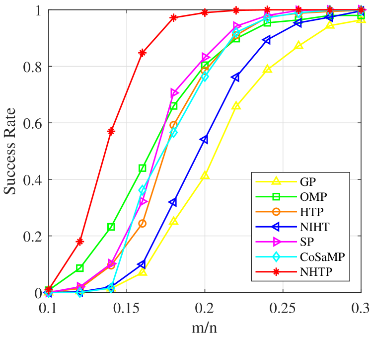
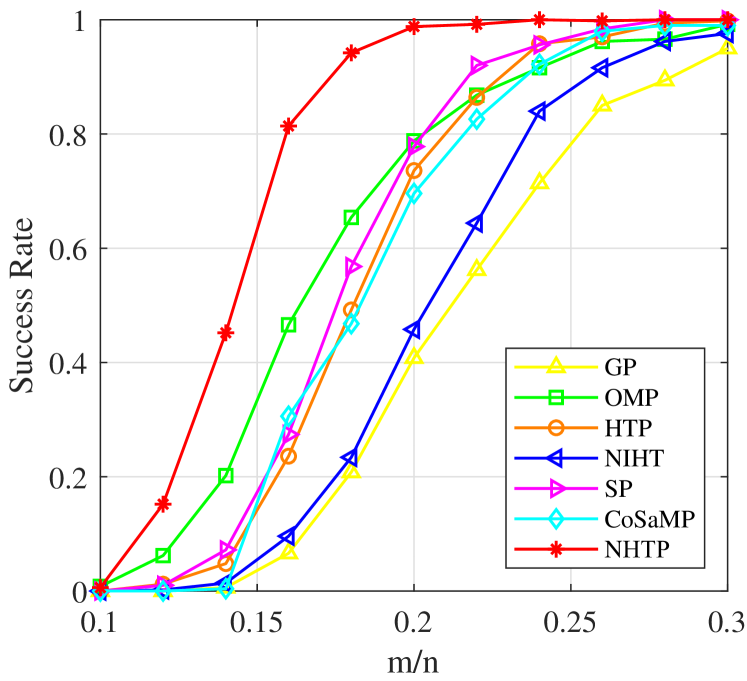
c) Numerical comparisons. We begin with running $500$ independent trials with fixed $n=256,m=\lceil n/4\rceil$ and recording the corresponding success rates (which is defined by the percentage of the number of successful recoveries over all trails) at sparsity levels $s$ from 6 to 36, where $\lceil a\rceil$ is the smallest integer that is no less than $a$. From Fig. 1, one can observe that for both Example 1 and Example 2, NHTP yielded the highest success rate for each $s$. For example, when $s=22$ for Gaussian matrix, our method still obtained $90\%$ successful recoveries while the other methods only guaranteed less than $40\%$ successful ones. Moreover, OMP, SP and HTP generated similar results, and GP and NIHT always came the last. Next we run $500$ independent trials with fixing $n=256,s=\lceil 0.05n\rceil$ but varying $m=\lceil rn\rceil$ where $r\in\{0.1,0.12,\cdots,0.3\}$. It is clearly to be seen that the larger $m$ is, the easier the problem becomes to be solved. This is illustrated by Fig. 2. Again NHTP outperformed the others due to highest success rate for each $s$, and GP and NIHT still came the last.

(a) Gaussian Matrix

(b) Partial DCT Matrix

Figure 1: Success rates. $n=256,m=\lceil n/4\rceil,s\in\{6,8,\cdots,36\}$.

(a) Gaussian Matrix

(b) Partial DCT Matrix

Figure 2: Success rates. $n=256,s=\lceil 0.05n\rceil,m=\lceil rn\rceil$ with $r\in\{0.1,0.12,\cdots,0.3\}$.

To see the accuracy of the solutions and the speed of these seven methods, we now run 50 trials for each kind of matrices with higher dimensions $n$ increasing from 5000 to 25000 and keeping $m=\lceil n/4\rceil,s=\lceil 0.01n\rceil,\lceil 0.05n\rceil$. Specific results produced by these seven methods are recorded in Tables 2 and 3. Our method NHTP always obtained the most accurate recovery, with accuracy order of $10^{-14}$ or higher, followed by HTP. NIHT was stable at achieving the solutions with accuracy of order $10^{-7}$. Moreover, GP and OMP rendered solutions as accurate as those by NHTP when $s=\lceil 0.01n\rceil$, but yielded inaccurate ones when $s=\lceil 0.05n\rceil$, which means that these two methods worked well when the solution is very sparse. In contrast, SP and CoSaMP always generated results with worst accuracy. When it comes to the computational speed in Table 3, NHTP is the fastest for most of the cases. The fast convergence of NHTP becomes more superior in high dimensional data setting. For example, when $n=25000$ and $s=\lceil 0.05n\rceil$, 6.58 seconds by NHTP against 36.93 seconds by HTP, which is the fastest method among the other five methods. GP and OMP always ran the slowest. In addition, we also compared seven algorithms on Example 1, but omitted all the related results since they were similar to those of Example 2

Table 2: Average absolute error $\|\mathbf{x}-\mathbf{x}^{*}\|$ for Example 2.

$s$	$n$	GP	OMP	HTP	NIHT	SP	CoSaMP	NHTP
$\lceil 0.01n\rceil$	5000	2.78e-15	2.40e-15	2.97e-15	2.42e-7	1.12e-5	1.12e-5	4.59e-16
	10000	5.21e-15	4.75e-15	5.70e-15	3.26e-7	3.59e-5	3.59e-5	1.10e-15
	15000	7.05e-15	7.07e-15	7.36e-15	4.28e-7	4.25e-5	4.25e-5	1.39e-15
	20000	9.49e-15	9.06e-15	9.47e-15	4.88e-7	6.56e-5	6.56e-5	1.88e-15
	25000	1.15e-14	1.12e-14	1.11e-14	5.32e-7	1.78e-4	1.78e-4	2.47e-15
$\lceil 0.05n\rceil$	5000	1.28e-03	1.40e-03	1.26e-14	4.80e-7	9.07e-5	9.07e-5	5.94e-15
	10000	7.91e-04	3.56e-04	2.44e-14	6.86e-7	1.77e-4	1.77e-4	1.18e-14
	15000	1.10e-03	6.20e-04	3.57e-14	8.54e-7	2.11e-4	2.11e-4	1.76e-14
	20000	9.43e-04	3.33e-04	4.87e-14	9.80e-7	3.53e-4	3.53e-4	2.39e-14
	25000	1.24e-03	5.57e-04	5.94e-14	1.01e-6	2.59e-4	2.59e-4	2.86e-14

Table 3: Average CPU time (in seconds) for Example 2.

$s$	$n$	GP	OMP	HTP	NIHT	SP	CoSaMP	NHTP
$\lceil 0.01n\rceil$	5000	0.69	0.48	0.09	0.30	0.07	0.05	0.06
	10000	4.47	3.70	0.33	1.21	0.31	0.25	0.16
	15000	14.57	13.41	0.74	2.96	0.96	0.86	0.37
	20000	32.70	30.46	1.34	5.53	2.30	2.00	0.65
	25000	68.94	67.13	2.49	37.03	20.11	4.18	1.13
$\lceil 0.05n\rceil$	5000	3.52	3.22	0.23	1.29	0.90	1.43	0.28
	10000	19.84	23.55	1.52	4.63	6.02	15.56	0.79
	15000	67.79	77.30	7.25	10.43	23.03	60.87	2.20
	20000	151.28	177.00	18.02	18.70	58.20	148.83	3.49
	25000	312.57	363.44	36.93	78.69	153.52	307.53	6.58

4.2 Sparse Logistic Regression

Sparse logistic regression (SLR) has drawn extensive attention since it was first proposed by Tibshirani (1996). Same as (Bahmani et al., 2013), we will address the so-called $\ell_{2}$ norm regularized sparsity constrained logistic regression (SCLR) model, namely,

$$\min_{\|\mathbf{x}\|_{0}\leq s}~{}~{}\ell(\mathbf{x})+\mu\|\mathbf{x}\|_{2}^{2}~{}~{}~{}~{}~{}~{}~{}~{}{\rm with}~{}~{}~{}~{}~{}~{}\ell(\mathbf{x}):=\frac{1}{m}\sum_{i=1}^{m}\left\{\ln(1+e^{\langle\mathbf{a}_{i},\mathbf{x}\rangle})-b_{i}\langle\mathbf{a}_{i},\mathbf{x}\rangle\right\},$$ (36)

where $\mathbf{a}_{i}\in\mathbb{R}^{n},b_{i}\in\{0,1\},i=1,\ldots,m$ are respectively given $m$ features and responses/labels, and $\mu>0$ (e.g. $\mu=10^{-6}/m$). The employment of a regularization was well justified because otherwise ‘one can achieve arbitrarily small loss values by tending the parameters to infinity along certain directions’ (see (Bahmani et al., 2013)). This is the reason why we will only focus on (36).

d) Testing examples. We will test three types of data sets. The first two are synthetic and the last one is from a real database. One synthetic data is adopted from (Lu and Zhang, 2013), (Pan et al., 2017) with the features $[\mathbf{a}_{1}~{}\cdots~{}\mathbf{a}_{m}]$ being generated identically and independently. The other is the same as Agarwal et al. (2010) or Bahmani et al. (2013) who have considered independent features with each $\mathbf{a}_{i}$ being generated by an autoregressive process (Hamilton, 1994).

Example 3 (Independent Data (Lu and Zhang, 2013; Pan et al., 2017))

To generate data labels $\mathbf{b}\in\{0,1\}^{m}$, we first randomly separate $\{1,\ldots,m\}$ into two parts $I$ and $I^{c}$ and set $b_{i}=0$ for $i\in I$ and $b_{i}=1$ for $i\in I^{c}$. Then the feature data is produced by

$$\mathbf{a}_{i}=y_{i}v_{i}\textbf{1}+\mathbf{w}_{i},\ \ \ \ i=1,\ldots,m$$

with $\mathbb{R}\ni~{}v_{i}\sim\mathcal{N}(0,1)$, $\mathbb{R}^{n}\ni\mathbf{w}_{i}\sim\mathcal{N}(0,\mathcal{I}_{n})$ and $\mathcal{N}(0,\mathcal{I}_{n})$ is the normal distribution with zero mean and the identity covariance. Since the sparse parameter $\mathbf{x}^{*}\in\mathbb{R}^{n}$ is unknown, different sparsity level$s$ will be tested.

Example 4 (Correlated Data (Agarwal et al., 2010; Bahmani et al., 2013))

The
sparse parameter $\mathbf{x}^{*}\in\mathbb{R}^{n}$ has $s$ nonzero entries drawn independently from the standard Gaussian distribution. Each data sample $\mathbf{a}_{i}=[a_{i1}~{}\cdots~{}a_{in}]^{\top},i=1,\ldots,m$ is an independent instance of the random vector generated by an autoregressive process (see Hamilton, 1994)

$$a_{i(j+1)}=\theta a_{ij}+\sqrt{1-\eta^{2}}v_{ij},\quad j=1,\ldots,n-1,$$

with $a_{i1}\sim\mathcal{N}(0,1)$, $v_{ij}\sim\mathcal{N}(0,1)$ and $\theta\in[0,1]$ being the correlation parameter. The data labels $\mathbf{y}\in\{0,1\}^{m}$ are then drawn randomly according to the Bernoulli distribution with

$${\rm Pr}\{y_{i}=0|\mathbf{a}_{i}\}=\left[1+e^{\langle\mathbf{a}_{i},\mathbf{x}^{*}\rangle}\right]^{-1},\ \ \ \ i=1,\ldots,m.$$

Example 5 (Real data)

This example comprises of seven real data sets for binary classification. They are colon-cancer, arcene, newsgroup, news20.binary1, duke breast- cancer1, leukemia1, rcv1.binary1, which are summarized in the following table, where the last three data sets have testing data. Moreover, as described in the website1, for the four data with small sample sizes: colon-cancer, arcene, duke breast-cancer and leukemia, sample-wise normalization has been conducted so that each sample has mean zero and variance one, and then feature-wise normalization has been conducted so that each feature has mean zero and variance one. For the rest four data with larger sample sizes, they are feature-wisely scaled to $[-1,1]$. All $-1$s in classes $\mathbf{b}$ are replaced by 0.

Data name	$m$ samples	$n$ features	training size $m_{1}$	testing size $m_{2}$
colon-cancer	62	2000	62	0
arcene	100	10000	100	0
newsgroup	11314	777811	11314	0
news20.binary	19996	1355191	19996	0
duke breast-cancer	42	7129	38	4
leukemia	72	7129	38	34
rcv1.binary	40242	47236	20242	20000

e) Benchmark methods. Since there are numerous leading solvers that have been proposed to solve SLR problems, we again only focus on those dealing with the $\ell_{2}$ norm regularized SCLR. We select three solvers: GraSP (Bahmani et al., 2013), NTGP (Yuan and Liu, 2014) and IIHT (Pan et al., 2017). Notice that all those methods are used to solve $\ell_{2}$ norm regularized SCLR model (36) with $\mu=10^{-6}/m$. Except for IIHT, which only used the first order information such as objective values or gradients, the other three methods exploit second order information of the objective function. NTGP integrates Newton directions into some steps, and GraSP takes advantage of the Matlab built-in function: minFunc which calls a Quasi-Newton strategy. For GraSP, if we use its defaults parameters, it would be less likely to meet its stopping criteria before the number of iteration reaching the maximal one. Compared with other three methods, which all generate a sequence with decreasing objective function values, the objective function value at each iteration by GraSP fluctuated greatly. Therefore, we set an extra stopping criterion for GraSP: $f(\mathbf{x}^{k})-f(\mathbf{x}^{k+1})<10^{-6}$. And if $f(\mathbf{x}^{k})<f(\mathbf{x}^{k+1})$, then terminate it and output $\mathbf{x}^{k}$. For NTGP, to facilitate its computational speed, we set maxIter=20 for outer loops, and maxIter$\_$sub=50 and optTol$\_$sub $=10^{-3}$ for inner loops. For IIHT, we keep its default parameters.

For both Example 3 and Example 4, we run $500$ independent trials if $n<10^{3}$ and $50$ independent trials otherwise, and report the average logistic loss $\ell(\mathbf{x})$ and CPU time to demonstrate the performance of each method.

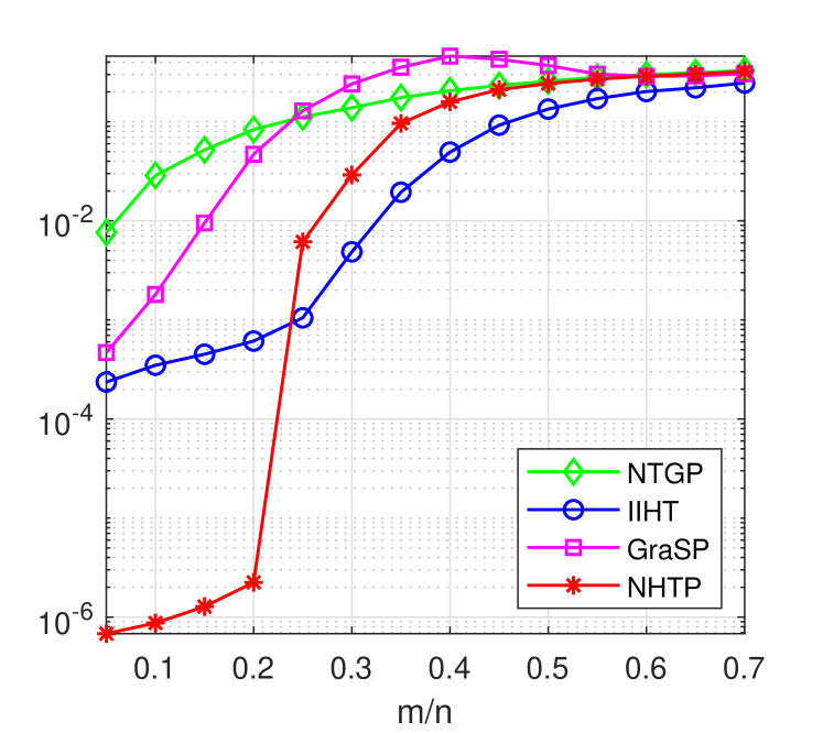
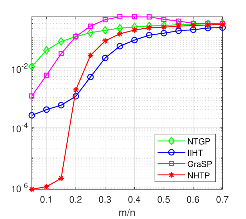
f) Numerical comparisons. For Example 3, we begin with testing each method for the case $n=256$ and $m=\lceil n/5\rceil$ with varying sparsity levels $s$ from 10 to 30. From Fig. 3(a), one can observe that IIHT rendered the best $\ell(\mathbf{x})$ when $s=10$ and NHTP performed the best $\ell(\mathbf{x})$ when $s>10$. And importantly, the value $\ell(\mathbf{x})$ produced by NHTP for each instance is far smaller than others, with order about $10^{-6}$. We then test the case $n=256,s=\lceil 0.05n\rceil$ and $m=\lceil rn\rceil$ with varying $r\in\{0.05,0.1,\cdots,0.7\}$. From Fig. 3(b), $\ell(\mathbf{x})$ generated by NHTP  is the lowest when the sample size was relatively small, and it gradually approached to the values similar to those obtained by the others. IIHT performed the best in terms of $\ell(\mathbf{x})$ when $m/n>0.2$ and GraSP always rendered the highest loss.

(a)  

(b)  

Figure 3: Average logistic loss $\ell(\mathbf{x})$ of four methods for Example 3.

Table 4: Average logistic loss $\ell(\mathbf{x})$ and CPU time (in seconds) for Example 3.

$s$	$n$	$\ell(\mathbf{x})$				CPU Time
		NTGP	IIHT	GraSP	NHTP	NTGP	IIHT	GraSP	NHTP
$\lceil 0.01n\rceil$	10000	2.39e-1	1.43e-1	2.44e-1	2.26e-1	8.403	1.723	0.488	0.313
	15000	2.48e-1	1.37e-1	2.39e-1	2.28e-1	17.81	3.307	0.974	0.457
	20000	2.35e-1	1.36e-1	2.36e-1	2.20e-1	32.61	6.245	1.862	0.842
	25000	2.25e-1	1.29e-1	2.30e-1	2.11e-1	52.99	8.913	3.006	1.372
	30000	2.24e-1	1.24e-1	2.30e-1	2.07e-1	76.31	14.15	4.309	2.140
	35000	2.21e-1	1.23e-1	2.29e-1	2.08e-1	149.7	21.84	16.08	2.875
	40000	2.18e-1	1.21e-1	2.32e-1	2.05e-1	466.1	29.12	804.2	3.923
$\lceil 0.05n\rceil$	10000	4.58e-2	4.76e-4	4.97e-3	6.50e-7	9.931	3.094	1.795	0.987
	15000	4.05e-2	4.69e-4	7.77e-3	3.32e-7	26.34	6.218	4.069	2.442
	20000	4.10e-2	4.80e-4	8.24e-3	6.32e-7	51.29	10.69	5.695	4.315
	25000	4.56e-2	4.90e-4	6.06e-3	4.77e-7	54.96	15.93	8.964	7.004
	30000	4.17e-2	4.92e-4	6.49e-3	6.89e-7	85.22	23.54	11.79	11.15
	35000	3.95e-2	4.89e-4	6.46e-3	6.65e-7	182.1	35.97	24.34	17.25
	40000	3.84e-2	4.92e-4	7.54e-3	5.81e-7	551.1	55.00	619.5	25.41

When the size of example is becoming relatively large, the picture is significant different. Hence we now run 50 independent trials with higher dimensions $n$ increasing from 10000 to 40000 and keeping $m=\lceil n/5\rceil,s=\lceil 0.01n\rceil,\lceil 0.05n\rceil$. As presented in Table 4, when $s=\lceil 0.01n\rceil$, IIHT produced the lowest $\ell(\mathbf{x})$, followed by NHTP which was the fastest. But when $s=\lceil 0.05n\rceil$, NHTP outperformed others in terms of $\ell(\mathbf{x})$ with order of $10^{-7}$ which was much better than others. The time used by NHTP is also significantly less than the others, for example, 25.41s by NHTP vs. 619.5s by GraSP when $n=40000$.

(a)  

(b)  

Figure 4: Average logistic loss $\ell(\mathbf{x})$ of four methods for Example 4.

Table 5: Average logistic loss $\ell(\mathbf{x})$ and CPU time (in seconds) for Example 4.

$s$	$n$	$\ell(\mathbf{x})$				CPU Time
		NTGP	IIHT	GraSP	NHTP	NTGP	IIHT	GraSP	NHTP
$\lceil 0.01n\rceil$	10000	1.87e-1	5.68e-2	1.93e-1	1.51e-1	8.338	4.394	0.471	0.245
	15000	1.81e-1	4.07e-2	1.73e-1	1.25e-1	19.72	7.156	1.403	0.702
	20000	1.61e-1	3.39e-2	1.64e-1	9.94e-2	36.68	10.74	2.370	1.194
	25000	1.62e-1	2.62e-2	1.61e-1	9.84e-2	54.37	16.51	3.800	1.922
	30000	1.63e-1	2.75e-2	1.63e-1	9.59e-2	124.4	40.11	18.83	6.067
	35000	1.58e-1	2.09e-2	1.52e-1	8.73e-2	179.1	44.47	199.2	8.257
	40000	1.59e-1	2.14e-2	1.57e-1	8.87e-2	423.4	46.13	639.4	19.47
$\lceil 0.05n\rceil$	10000	7.59e-2	6.02e-4	2.18e-2	1.54e-6	9.101	3.426	1.875	0.880
	15000	7.95e-2	6.15e-4	2.02e-2	1.67e-6	20.40	7.426	4.316	2.140
	20000	7.84e-2	5.93e-4	2.34e-2	1.55e-6	34.91	12.51	6.394	4.015
	25000	7.96e-2	5.97e-4	2.44e-2	1.65e-6	54.41	19.03	8.921	6.590
	30000	7.76e-2	6.00e-4	2.04e-2	1.58e-6	107.2	29.95	16.57	10.09
	35000	7.74e-2	6.01e-4	2.18e-2	1.61e-6	137.3	45.71	26.05	16.10
	40000	7.89e-2	5.90e-4	2.41e-2	1.58e-6	305.8	70.83	721.0	22.46

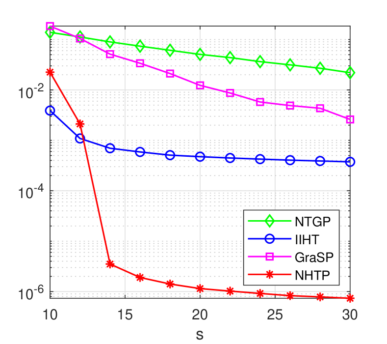
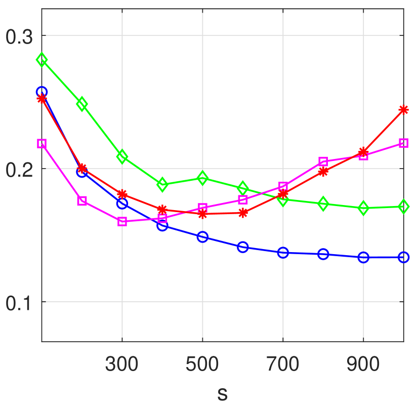
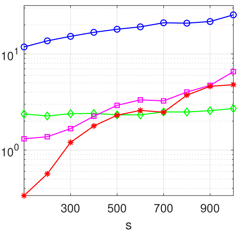
For Example 4, it is related to the parameter $\theta$. We only report the results for $\theta=1/2$ since the comparisons of all methods are similar for each fixed $\theta\in(0,1)$. Again we first fix $n=256,m=\lceil n/5\rceil$ and vary sparsity levels $s$ from 10 to 30. As shown in Fig. 4 (a), NHTP yielded the smallest logistic loss when $s>12$, followed by IIHT. We then fix $n=256,s=\lceil 0.05n\rceil$ and change the sample size $m=\lceil rn\rceil$, where $r\in\{0.05,0.1,0.15,\cdots,0.7\}$. From Fig. 4(b), NHTP outperformed others when the sample size was relatively small such as $m/n<0.2$, while IIHT performed best in terms of $\ell(\mathbf{x})$ when $m/n\geq 0.2$.

When the size of the example is becoming relatively large, the picture again is significant different. We run 50 independent trials with higher dimensions $n$ increasing from 10000 to 40000 and keeping $m=\lceil n/5\rceil,s=\lceil 0.01n\rceil,\lceil 0.05n\rceil$. As presented in Table 5, when $s=\lceil 0.01n\rceil$ IIHT indeed provided the best logistic loss and comparable to ours. However, NHTP was significantly faster than IIHT. Clearly, under the case of $s=\lceil 0.05n\rceil$, NHTP offered the far lowest $\ell(\mathbf{x})$ with order of $10^{-6}$ and CPU time with 22.46 seconds against 721 seconds from GraSP when $n=40000$.

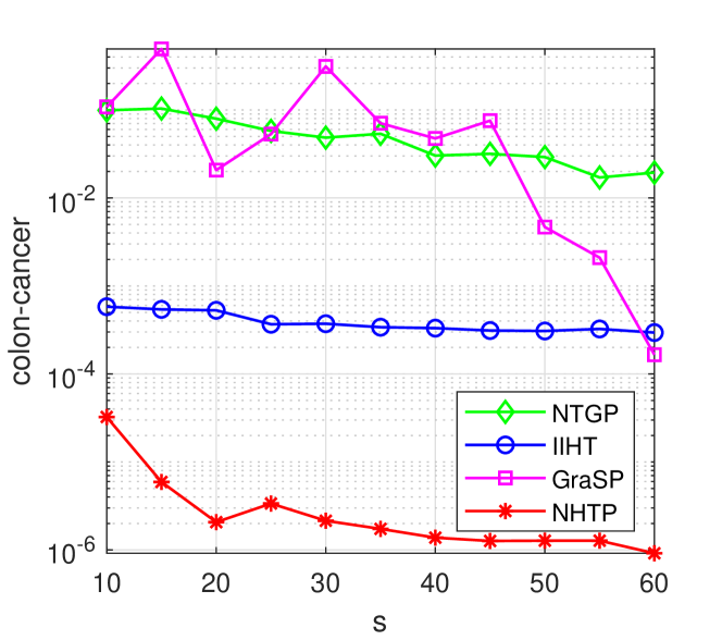
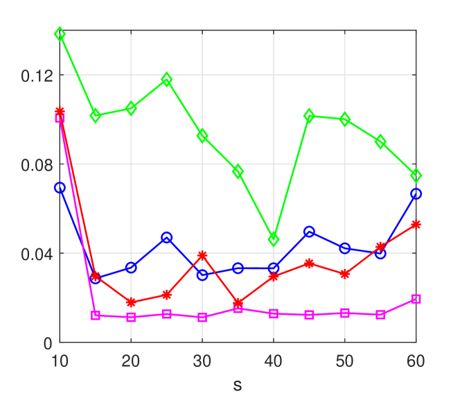
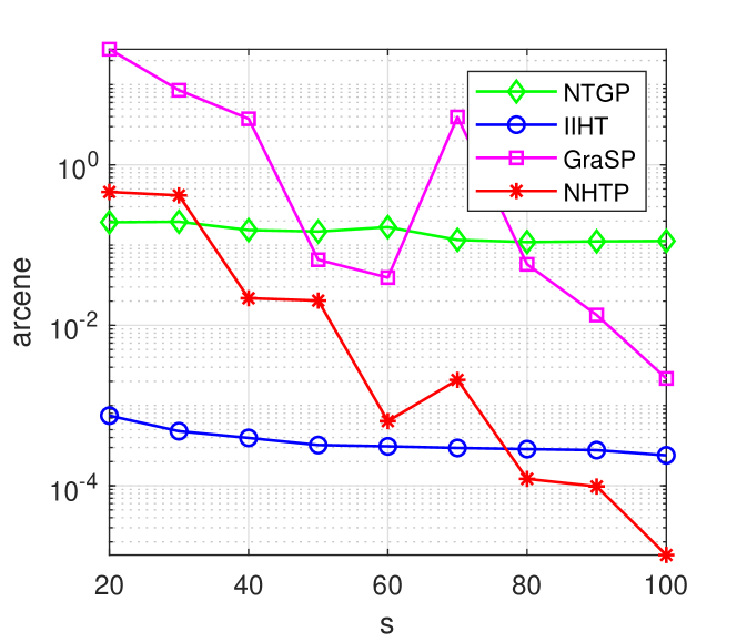
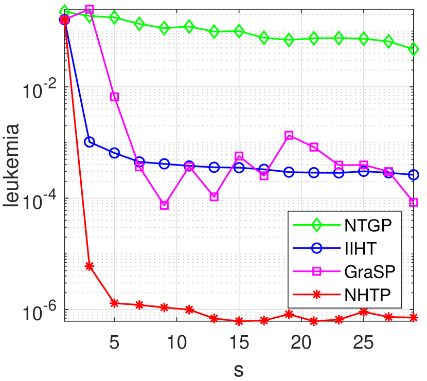
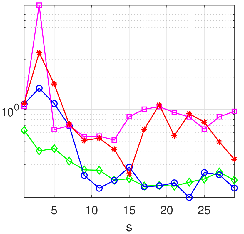
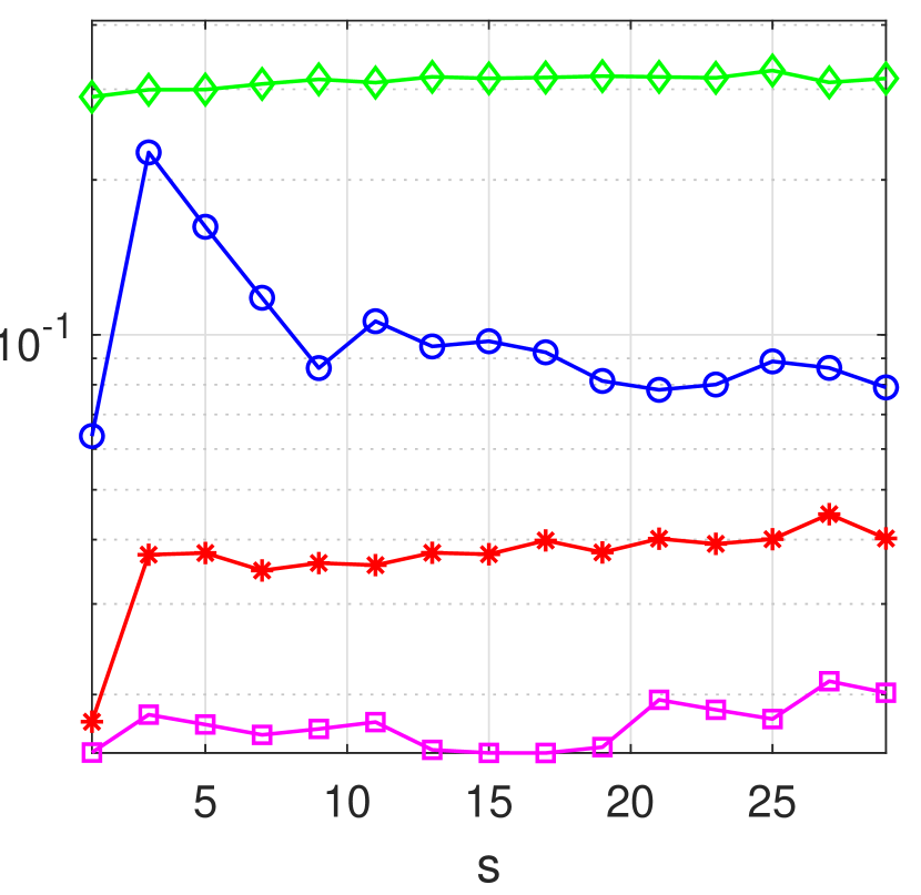
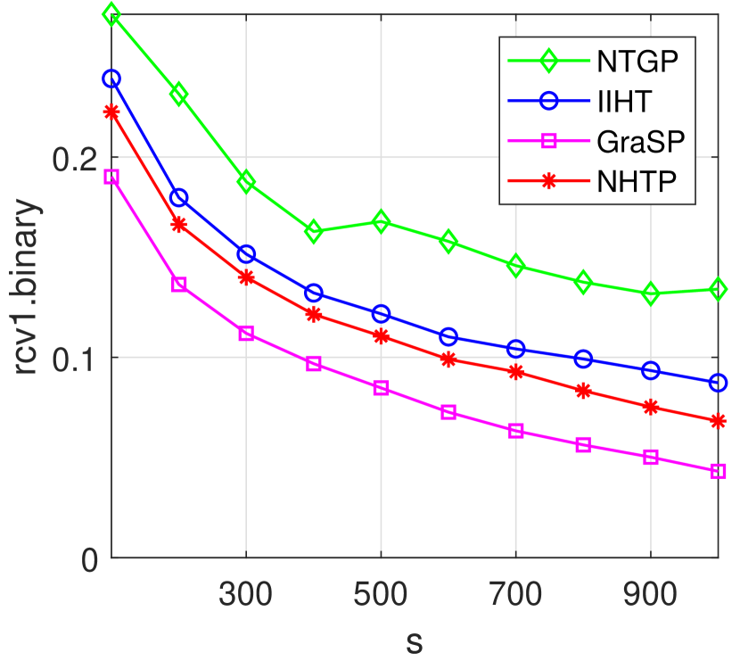
Now we compare these four methods on solving real data in Example 5. For each method, we demonstrate its performance on instances with varying $s$. We first illustrate the performance of each method on solving those data without testing data sets. As presented in Fig. 5, we have the following observations:

• For colon-cancer, NHTP obtained the smallest $\ell(\mathbf{x})$ followed by IIHT. While GraSP ran the fastest and NTGP performed the slowest.

• For arcene, IIHT and NHTP generated best $\ell(\mathbf{x})$ when $s<80$ and $s\geq 80$ respectively. And the latter consumed the smallest CPU time.

• For newsgroup, NHTP outperformed others in terms of the smallest $\ell(\mathbf{x})$ and CPU time. NTGP rendered the worst logistic loss and IIHT ran the slowest.

• For news20.binary, GraSP performed unstably, yet achieving best $\ell(\mathbf{x})$ for some cases such as $s\leq 1300$. NTGP still produced the highest logistic loss. As for computational speed, NHTP was the fastest and IIHT was the slowest.

(a) $\ell(\mathbf{x})$

(b) CPU time

(c) $\ell(\mathbf{x})$

(d) CPU time

(e) $\ell(\mathbf{x})$

(f) CPU time

(g) $\ell(\mathbf{x})$

(h) CPU time

Figure 5: Logistic loss $\ell(\mathbf{x})$ and CPU time of four methods for Example 5.

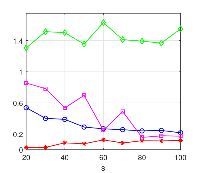
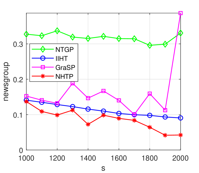
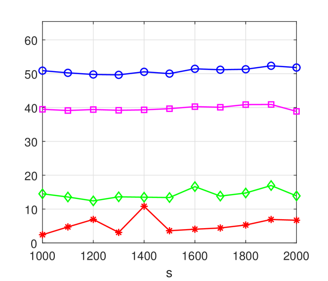
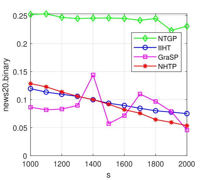
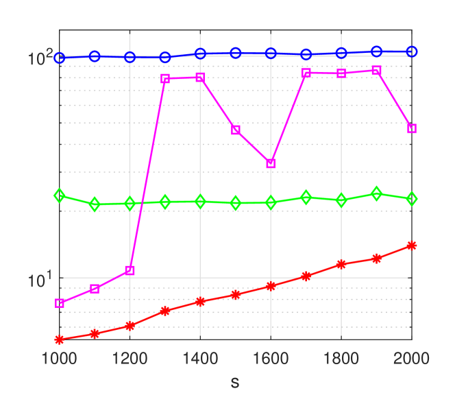
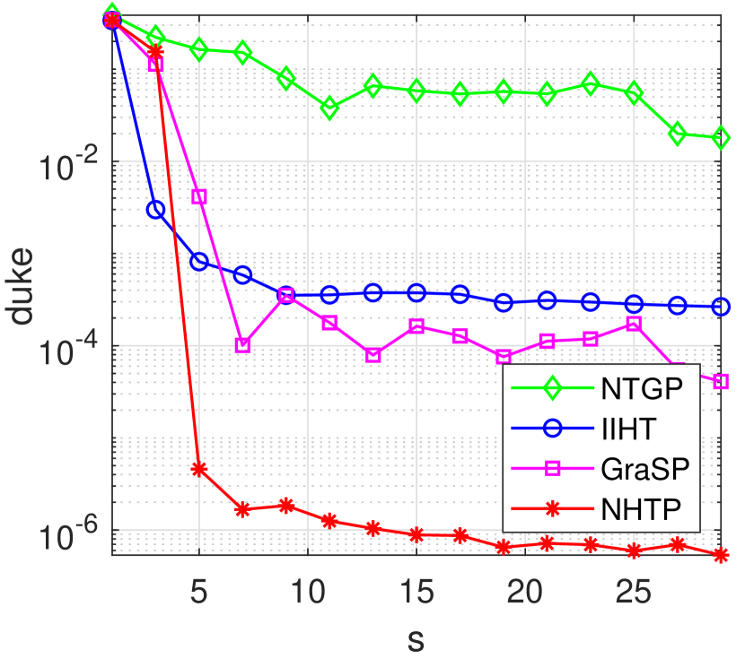
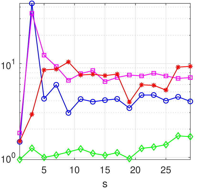
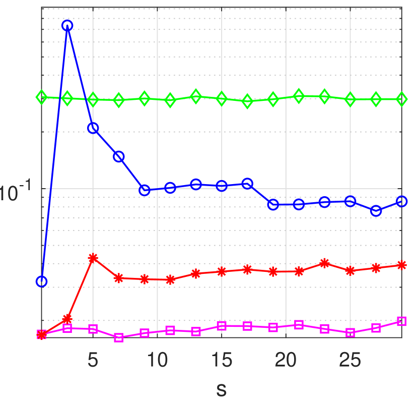
Next we illustrate the performance of each method on solving those data with testing data sets. As shown in Fig. 6, some comments are able to be made as follows:

• For duke breast-cancer, along with increasing $s$, $\ell(\mathbf{x})$ on training data obtained by NHTP dropped significantly, with order $10^{-6}$. By contrast, NTGP stabilized at above $10^{-2}$. When it comes to the testing data, apparently NTGP yielded the best $\ell(\mathbf{x})$, followed by IIHT. It seems that the higher $\ell(\mathbf{x})$ on training data was solved by a method, the lower $\ell(\mathbf{x})$ on testing data would be provided. For CPU time, GraSP behaved the fastest, followed by NHTP, IIHT and NTGP.

• For leukemia, the performance of each method was similar to that on duke breast- cancer data. A slightly difference was that NTGP no more offered the best $\ell(\mathbf{x})$ on testing data as IIHT generated the best ones for some $s$.

• For rcv1.binary, GraSP performed the best $\ell(\mathbf{x})$ on training data, followed by our method. Again NTGP came the last. It is obvious that IIHT got the smallest $\ell(\mathbf{x})$ on testing data when $s\geq 400$, while GraSP produced the best ones otherwise. For CPU time, NHTP and NTGP was the most efficient when $s\geq 600$ and $s>600$ respectively.

(a) Training $\ell(\mathbf{x})$

(b) Testing $\ell(\mathbf{x})$

(c) CPU time

(d) Training $\ell(\mathbf{x})$

(e) Testing $\ell(\mathbf{x})$

(f) CPU time

(g) Training $\ell(\mathbf{x})$

(h) Testing $\ell(\mathbf{x})$

(i) CPU time

Figure 6: Logistic loss $\ell(\mathbf{x})$ and CPU time of four methods for Example 5.

5 Conclusion and Future Research

There exists numerous papers that use a restricted Newton step to accelerate methods belonging to hard-thresholding pursuits. This results in the method of Newton hard-thresholding pursuit. On the one hand, existing empirical experience shows significance acceleration when Newton’s step is employed . On the other hand, existing theory for such methods does not offer any better statistical guarantee than the simple hard thresholding counterparts. The discrepancy between the superior empirical performance and the no-better theoretical guarantee has been well documented in the case of CS problem (2) and it invites further theory for justification.

In this paper, we develop a new NHTP, which makes use of the strategy “approximation and restriction” to obtain the truncated approximation within a subspace. This is in contrast to the popular strategy “restriction and approximation”. We note that both strategies lead to the same Newton step in the case of CS. We further cast the resulting Newton step as a Newton iteration for a nonlinear equation. This new interpretation of the Newton step provides a new route for establishing its quadratic convergence. Finally, we used the Armijo line search to globalize the method. Extensive numerical experiments confirm the efficiency of the proposed method. The global and quadratic convergence theory for NHTP offers a theoretical justification why such methods are more efficient than their simple hard thresholding counterparts. There are a few of topics that are worth exploring further.

• We expect that our algorithmic framework will make it possible to study quadratic convergence of existing NHTP based on the strategy of “restriction and approximation”. A plausible approach would be to regard such method as an inexact version of our NHTP. Technically, it would involve quantifying/controlling the inexactness so as to ensure the quadratic convergence to hold.

• As rightly pointed out by one referee, “the proof technique revolves around providing sufficient conditions for descent (and reverting to standard gradient descent when descent does not hold). However, there are many methods that are non-descent and convergence still does hold. Blumensath’s method in Blumensath (2012) (or acceleration in general) is one such method wherein it has been observed in practice in subsequent works that the existence of a ‘ripple’ effect, akin to other accelerated methods wherein descent is not required for overall convergence.” In our numerical experiments, we also observed that the provided sufficient conditions for descent are not necessary. But it will be curious to see if the descent itself is necessary, while enjoying the stated convergence.

• We proved in Thm. 10 that quadratic convergence takes place after certain $k_{0}$ iterations. It would be nice to estimate and quantify how big this $k_{0}$ would be. Such research belongs to computational complexity in optimization. We plan to investigate all of those in future.

Acknowledgement. We sincerely thank the associate editor and the two referees for their detailed comments that have helped us to improve the paper. We particularly thank the referee who went through our technical proofs and offered us valuable suggestions on the condition (16). We also thank Prof Ziyan Luo of Beijing Jiaotong University, who helped us to improve the proof of Thm. 10.

A Identities and Inequalities for Proofs

Due to the restricted fashion of NHTP, we need to keep tracking the indices belonging to the subspace $\mathbf{x}|_{T_{k}}=0$ and also those fall out of this subspace. To simplify our proofs, we will use a few more abbreviations and derive some identities and inequalities associated with the Newton direction $\mathbf{d}^{k}_{N}$. The sequence $\{\mathbf{x}^{k}\}$ used is generated by NHTP.

(a) Simplification of Newton’s equation (20). We first define

$$J_{k}:=T_{k-1}\setminus T_{k},\qquad H_{k}:=\nabla_{{T_{k}}}^{2}f(\mathbf{x}^{k}),\qquad G_{k}:=\nabla_{{T_{k}},{J_{k}}}^{2}f(\mathbf{x}^{k}).$$ (37)

We also have the following easy observation:

$$\mbox{supp}(\mathbf{x}^{k})\subseteq T_{k-1},\quad|T_{k}|=|T_{k-1}|=s,\quad\mbox{and}\quad|T_{k}\setminus T_{k-1}|=|T_{k-1}\setminus T_{k}|=|J_{k}|.$$ (38)

It is important to note that $\mathbf{x}^{k}_{T_{k}^{c}}$ is also $s$-sparse. This is because for any $i\not\in T_{k-1}$, $x^{k}_{i}=0$ (because $\mbox{supp}(\mathbf{x}^{k})\subseteq T_{k-1}$),

$$\mathbf{x}^{k}_{T_{k}^{c}}=\left[\begin{array}[]{c}\mathbf{x}^{k}_{T_{k}^{c}\cap T_{k-1}}\\[2.58334pt] 0\end{array}\right]=\left[\begin{array}[]{c}\mathbf{x}^{k}_{T_{k-1}\setminus T_{k}}\\[2.58334pt] 0\end{array}\right]=\left[\begin{array}[]{c}\mathbf{x}^{k}_{J_{k}}\\[2.58334pt] 0\end{array}\right],$$ (39)

and $|J_{k}|\leq|T_{k-1}\setminus T_{k}|\leq|T_{k-1}|=s$. We emphasize that $J_{k}$ captures all nonzero elements in $\mathbf{x}^{k}_{T_{k}^{c}}$. Therefore, we will see more $J_{k}$ instead of $T_{k}^{c}$ being used in our derivation below. This observation leads to the simplified Newton equation of (20):

$$\left\{\begin{array}[]{rcl}H_{k}(\mathbf{d}_{N}^{k})_{T_{k}}&=&G_{k}\mathbf{x}^{k}_{J_{k}}-\nabla_{T_{k}}f(\mathbf{x}^{k})\\[6.45831pt] (\mathbf{d}_{N}^{k})_{T^{c}_{k}}&=&-\mathbf{x}^{k}_{{T}_{k}^{c}}=-\left[\begin{array}[]{c}\mathbf{x}^{k}_{J_{k}}\\[2.58334pt] 0\end{array}\right].\end{array}\right.$$ (40)

An important feature to note is that the vectors $(\mathbf{d}_{N}^{k})_{T_{k}}$, $(\mathbf{d}_{N}^{k})_{T^{c}_{k}}$, $\mathbf{x}^{k}_{J_{k}}$ are all $s$-sparse. Putting together, at each iteration, we only involve vectors that do not exceed $2s$-sparsity. This is the reason why our assumptions are always on $2s$-restricted properties of $f$.

(b) An identity on the Newton direction. This involves a string of equalities as follows. We write $\mathbf{d}^{k}$ for $\mathbf{d}^{k}_{N}$ because there is no danger to cause any confusion.

$$\langle\mathbf{d}^{k}_{T_{k}\cup J_{k}},\nabla^{2}_{T_{k}\cup J_{k}}f(\mathbf{x}^{k})\mathbf{d}^{k}_{T_{k}\cup J_{k}}\rangle\qquad\quad(\mbox{note}\ {T_{k}\cap J_{k}}=\emptyset)$$

$$= \left[\begin{array}[]{cc}\mathbf{d}^{k}_{T_{k}}\\[2.58334pt] \mathbf{d}^{k}_{J_{k}}\end{array}\right]^{\top}\left[\begin{array}[]{cc}H_{k},&\ G_{k}\\[2.58334pt] G_{k}^{\top},&\ \nabla^{2}_{J_{k}}f(\mathbf{x}^{k})\end{array}\right]\left[\begin{array}[]{cc}\mathbf{d}^{k}_{T_{k}}\\[2.58334pt] \mathbf{d}^{k}_{J_{k}}\end{array}\right]$$

$$= \left[\begin{array}[]{cc}\mathbf{d}^{k}_{T_{k}}\\[2.58334pt] \mathbf{d}^{k}_{J_{k}}\end{array}\right]^{\top}\left[\begin{array}[]{c}H_{k}\mathbf{d}^{k}_{T_{k}}+G_{k}\mathbf{d}^{k}_{J_{k}}\\[2.58334pt] G_{k}^{\top}\mathbf{d}^{k}_{T_{k}}+\nabla^{2}_{J_{k}}f(\mathbf{x}^{k})\mathbf{d}^{k}_{J_{k}}\end{array}\right]$$

$$\overset{(\ref{Newton-Direction-2})}{=} \left[\begin{array}[]{cc}\mathbf{d}^{k}_{T_{k}}\\[2.58334pt] \mathbf{d}^{k}_{J_{k}}\end{array}\right]^{\top}\left[\begin{array}[]{c}-\nabla_{T_{k}}f(\mathbf{x}^{k})\\[2.58334pt] G_{k}^{\top}\mathbf{d}^{k}_{T_{k}}+\nabla^{2}_{J_{k}}f(\mathbf{x}^{k})\mathbf{d}^{k}_{J_{k}}\end{array}\right]$$

$$= -\langle\nabla_{T_{k}}f(\mathbf{x}^{k}),\mathbf{d}^{k}_{T_{k}}\rangle+\langle G_{k}\mathbf{d}^{k}_{J_{k}},\mathbf{d}^{k}_{T_{k}}\rangle+\langle\mathbf{d}^{k}_{J_{k}},\nabla^{2}_{J_{k}}f(\mathbf{x}^{k})\mathbf{d}^{k}_{J_{k}}\rangle$$

$$\overset{(\ref{Newton-Direction-2})}{=} -\langle\nabla_{T_{k}}f(\mathbf{x}^{k}),\mathbf{d}^{k}_{T_{k}}\rangle-\langle H_{k}\mathbf{d}^{k}_{T_{k}}+\nabla_{T_{k}}f(\mathbf{x}^{k}),\mathbf{d}^{k}_{T_{k}}\rangle+\langle\mathbf{d}^{k}_{J_{k}},\nabla^{2}_{J_{k}}f(\mathbf{x}^{k})\mathbf{d}^{k}_{J_{k}}\rangle$$

$$= -2\langle\nabla_{T_{k}}f(\mathbf{x}^{k}),\mathbf{d}^{k}_{T_{k}}\rangle-\langle H_{k}\mathbf{d}^{k}_{T_{k}},\mathbf{d}^{k}_{T_{k}}\rangle+\langle\mathbf{d}^{k}_{J_{k}},\nabla^{2}_{J_{k}}f(\mathbf{x}^{k})\mathbf{d}^{k}_{J_{k}}\rangle.$$

This leads to our identity:

$$2\langle\nabla_{T_{k}}f(\mathbf{x}^{k}),\ \mathbf{d}^{k}_{T_{k}}\rangle = -\langle\mathbf{d}^{k}_{T_{k}\cup J_{k}},\nabla^{2}_{T_{k}\cup J_{k}}f(\mathbf{x}^{k})\mathbf{d}^{k}_{T_{k}\cup J_{k}}\rangle$$ (44)

$$-\langle H_{k}\mathbf{d}^{k}_{T_{k}},\ \mathbf{d}^{k}_{T_{k}}\rangle+\langle\mathbf{d}^{k}_{J_{k}},\ \nabla^{2}_{J_{k}}f(\mathbf{x}^{k})\mathbf{d}^{k}_{J_{k}}\rangle.$$

(c) An inequality on the gradient sequence. The role of $T_{k}$ is like a working active set that is designed to identify the true support of an optimal solution. Its complementary set $T_{k}^{c}$ is handled in such a way to make sure the next iterate $\mathbf{x}^{k+1}$ has zeros on $T_{k}^{c}$. To achieve this, in both the Newton direction $\mathbf{d}^{k}_{N}$ and the gradient direction $\mathbf{d}^{k}_{g}$ we set

$$\Big{(}\mathbf{d}^{k}_{N}\Big{)}_{T_{k}^{c}}=\Big{(}\mathbf{d}^{k}_{g}\Big{)}_{T_{k}^{c}}=-\mathbf{x}^{k}_{T_{k}^{c}}.$$

Let $\mathbf{d}^{k}$ be either $\mathbf{d}_{N}^{k}$ or $\mathbf{d}^{k}_{g}$. It follows from (39) that

$$\begin{array}[]{l}\|\mathbf{x}^{k}_{T^{c}_{k}}\|=\|\mathbf{x}^{k}_{J_{k}}\|=\|\mathbf{d}^{k}_{J_{k}}\|=\|\mathbf{d}^{k}_{T^{c}_{k}}\|,\quad\|\mathbf{d}^{k}\|=\|\mathbf{d}^{k}_{T_{k}\cup J_{k}}\|\\[8.61108pt] \langle\nabla_{T^{c}_{k}}f(\mathbf{x}^{k}),\ \mathbf{x}^{k}_{T^{c}_{k}}\rangle=\langle\nabla_{J_{k}}f(\mathbf{x}^{k}),\ \mathbf{x}^{k}_{J_{k}}\rangle\end{array}$$ (45)

By the definition of $T_{k}$ and the fact, $x^{k}_{i}=0$ for $i\in T_{k}\setminus T_{k-1}$, we have

$$|\eta\nabla_{i}f(\mathbf{x}^{k})|^{2}=|x_{i}^{k}-\eta\nabla_{i}f(\mathbf{x}^{k})|^{2}\geq|x_{j}^{k}-\eta\nabla_{j}f(\mathbf{x}^{k})|^{2},\ \ \forall\ i\in T_{k}\setminus T_{k-1},\ \ j\in J_{k}.$$

The above inequality and the fact $|T_{k}\setminus T_{k-1}|=|J_{k}|$ in (38) imply

$$\eta^{2}\|\nabla_{T_{k}\setminus T_{k-1}}f(\mathbf{x}^{k})\|^{2}=\sum_{i\in T_{k}\setminus T_{k-1}}|\eta\nabla_{i}f(\mathbf{x}^{k})|^{2}\geq\sum_{j\in J_{k}}|x^{k}_{j}-\eta\nabla_{i}f(\mathbf{x}^{k})|^{2}$$

$$\geq \|\mathbf{x}^{k}_{J_{k}}-\eta\nabla_{J_{k}}f(\mathbf{x}^{k})\|^{2}=\|\mathbf{x}^{k}_{J_{k}}\|^{2}-2\eta\langle\mathbf{x}^{k}_{J_{k}},\ \nabla_{J_{k}}f(\mathbf{x}^{k})\rangle+\eta^{2}\|\nabla_{J_{k}}f(\mathbf{x}^{k})\|^{2}$$

$$\overset{(\ref{xk-Tc-T1})}{=} \|\mathbf{x}^{k}_{T^{c}_{k}}\|^{2}-2\eta\langle\mathbf{x}^{k}_{J_{k}},\ \nabla_{J_{k}}f(\mathbf{x}^{k})\rangle+\eta^{2}\|\nabla_{J_{k}}f(\mathbf{x}^{k})\|^{2},$$

which together with

$$\|\nabla_{T_{k}}f(\mathbf{x}^{k})\|^{2} = \|\nabla_{T_{k}\cap T_{k-1}}f(\mathbf{x}^{k})\|^{2}+\|\nabla_{T_{k}\setminus T_{k-1}}f(\mathbf{x}^{k})\|^{2}$$

$$\|\nabla_{T_{k-1}}f(\mathbf{x}^{k})\|^{2} = \|\nabla_{T_{k}\cap T_{k-1}}f(\mathbf{x}^{k})\|^{2}+\|\nabla_{J_{k}}f(\mathbf{x}^{k})\|^{2}$$

results in the following inequality on the gradient $\nabla f(\mathbf{x}^{k})$

$$\eta\|\nabla_{T_{k}}f(\mathbf{x}^{k})\|^{2}-\eta\|\nabla_{T_{k-1}}f(\mathbf{x}^{k})\|^{2}-\|\mathbf{x}^{k}_{T_{k}^{c}}\|^{2}/\eta\geq-2\langle\mathbf{x}^{k}_{J_{k}},\ \nabla_{J_{k}}f(\mathbf{x}^{k})\rangle.$$ (46)

B Proofs of all results

B.1 Proof of Lemma 4

Proof  The first claim is obvious and we onely prove the second one. The proof for the “only if” part is straightforward. Suppose $\mathbf{x}$ satisfies (10). We have $\mathbf{x}={\cal P}_{s}(\mathbf{x}-\eta\nabla f(\mathbf{x}))$. By the definition of ${\cal P}_{s}(\cdot)$ and $T\in{\cal T}(\mathbf{x},\eta)$, we have $\mathbf{x}_{T^{c}}=0$ and

$$\mathbf{x}_{T}=\Big{(}{\cal P}_{s}(\mathbf{x}-\eta\nabla f(\mathbf{x}))\Big{)}_{T}=(\mathbf{x}-\eta\nabla f(\mathbf{x}))_{T}=\mathbf{x}_{T}-\eta\nabla_{T}f(\mathbf{x}),$$

which implies $\nabla_{T}f(\mathbf{x})=0$.

We now prove the “if” part. Suppose we have $F_{\eta}(\mathbf{x};T)=0~{}~{}\text{for~{}all}~{}~{}T\in{\cal T}(\mathbf{x};\eta)$, namely,

$$\nabla_{T}f(\mathbf{x})=0,~{}~{}\mathbf{x}_{T^{c}}=0.$$ (47)

We consider two cases. Case I: ${\cal T}(\mathbf{x};\eta)$ is a singleton. By letting $T$ be the only element of ${\cal T}(\mathbf{x};\eta)$, then

$$\mathbf{x}-{\cal P}_{s}(\mathbf{x}-\eta\nabla f(\mathbf{x}))=\left[\begin{array}[]{c}\mathbf{x}_{T}\\ \mathbf{x}_{T^{c}}\end{array}\right]-\left[\begin{array}[]{c}\mathbf{x}_{T}-\eta\nabla_{T}f(\mathbf{x})\\ 0\end{array}\right]\overset{(\ref{zdt})}{=}\left[\begin{array}[]{c}\mathbf{x}_{T}-\mathbf{x}_{T}\\ 0-0\end{array}\right]=0,$$

which means $\mathbf{x}$ satisfies the fixed point equation (10).

Case II: ${\cal T}(\mathbf{x};\eta)$ has multiple elements. Then by the definition (12) of ${\cal T}(\mathbf{x};\eta)$ we have two claims:

$$(x-\eta\nabla f(\mathbf{x}))_{(s)}=(x-\eta\nabla f(\mathbf{x}))_{(s+1)}>0~{}~{}~{}~{}{\rm or}~{}~{}~{}~{}(x-\eta\nabla f(\mathbf{x}))_{(s)}=0.$$

Now we exclude the first claim. Without loss of any generality, we assume

$$|x_{1}-\eta\nabla_{1}f(\mathbf{x})|\geq\cdots\geq|x_{s}-\eta\nabla_{s}f(\mathbf{x})|=|x_{s+1}-\eta\nabla_{s+1}f(\mathbf{x})|=(x-\eta\nabla f(\mathbf{x}))_{(s)}.$$

Let $T_{1}=\{1,2,\cdots,s\}$ and $T_{2}=\{1,2,\cdots,s-1,s+1\}$. Then $F_{\eta}(\mathbf{x};T_{1})=F_{\eta}(\mathbf{x};T_{2})=0$ imply that $\nabla_{T_{1}}f(\mathbf{x})=\nabla_{T_{2}}f(\mathbf{x})=0$ and $\mathbf{x}_{T^{c}_{1}}=\mathbf{x}_{T^{c}_{2}}=0$, which lead to

$$|x_{1}| = |x_{1}-\eta\nabla_{1}f(\mathbf{x})|\geq\cdots\geq|x_{s}|=|x_{s}-\eta\nabla_{s}f(\mathbf{x})|=$$

$$|x_{s+1}| = |x_{s+1}-\eta\nabla_{s+1}f(\mathbf{x})|=(x-\eta\nabla f(\mathbf{x}))_{(s)}>0.$$

This is contradicted with $\mathbf{x}_{T^{c}_{1}}=0$ because of $(s+1)\in T^{c}_{1}$. Therefore, we have $(x-\eta\nabla f(\mathbf{x}))_{(s)}=0$. This together with the definition (12) of ${\cal T}(\mathbf{x};\eta)$ yields $0=(x-\eta\nabla f(\mathbf{x}))_{(s)}\geq|x_{i}-\eta\nabla_{i}f(\mathbf{x})|=|\eta\nabla_{i}f(\mathbf{x})|$ for any $i\in T^{c}$, which combining $\nabla_{T}f(\mathbf{x})=0$ renders $\nabla f(\mathbf{x})=0$. Hence $x_{(s)}=(x-\eta\nabla f(\mathbf{x}))_{(s)}=0$, yielding $\|\mathbf{x}\|_{0}<s$. Consequently, $\mathbf{x}=\mathbf{x}-\eta\nabla f(\mathbf{x})$ (because $\nabla f(\mathbf{x})=0$ and $\mathbf{x}={\cal P}_{s}(\mathbf{x})={\cal P}_{s}(\mathbf{x}-\eta\nabla f(\mathbf{x}))$ (because $\|\mathbf{x}\|_{0}<s$). That is $\mathbf{x}$ also satisfies the fixed point equation (10).  

B.2 Proof of Lemma 5

Proof  For simplicity, we write $\mathbf{d}^{k}:=\mathbf{d}^{k}_{N}$. Since $f(\mathbf{x})$ is $m_{2s}$-restricted strongly convex and $M_{2s}$-restricted strongly smooth. For any $\|\mathbf{x}\|_{0}\leq s$ , it follows from Definition 1 that

$$m_{2s}I_{2s}\preceq\nabla^{2}_{{T}}f(\mathbf{x})\preceq M_{2s}I_{2s}\hskip 28.45274pt{\rm for~{}any~{}}|T|\leq 2s.$$ (48)

Clearly, $|T_{k}\cup J_{k}|\leq 2s$ due to $|T_{k}|\leq s$ and $|J_{k}|\leq s$. This together with (44) implies

$$2\left\langle\nabla_{T_{k}}f(\mathbf{x}^{k}),\mathbf{d}^{k}_{T_{k}}\right\rangle = -\left\langle\mathbf{d}^{k}_{T_{k}\cup J_{k}},\nabla^{2}_{T_{k}\cup J_{k}}f(\mathbf{x}^{k})\mathbf{d}^{k}_{T_{k}\cup J_{k}}\right\rangle$$ (49)

$$-\left\langle H_{k}\mathbf{d}^{k}_{T_{k}},\mathbf{d}^{k}_{T_{k}}\right\rangle+\left\langle\mathbf{d}^{k}_{J_{k}},\nabla^{2}_{J_{k}}f(\mathbf{x}^{k})\mathbf{d}^{k}_{J_{k}}\right\rangle$$

$$\leq -m_{2s}\left[\|\mathbf{d}^{k}_{T_{k}\cup J_{k}}\|^{2}+\|\mathbf{d}^{k}_{T_{k}}\|^{2}\right]+M_{2s}\|\mathbf{x}^{k}_{T^{c}_{k}}\|^{2}$$

$$= -m_{2s}\left[\|\mathbf{d}^{k}_{T_{k}\cup J_{k}}\|^{2}+\|\mathbf{d}^{k}_{T_{k}}\|^{2}+\|\mathbf{d}^{k}_{J_{k}}\|^{2}-\|\mathbf{d}^{k}_{J_{k}}\|^{2}\right]+M_{2s}\|\mathbf{x}^{k}_{T^{c}_{k}}\|^{2}$$

$$\overset{(\ref{xk-Tc-T1})}{=} -2m_{2s}\|\mathbf{d}^{k}\|^{2}+m_{2s}\|\mathbf{x}^{k}_{T^{c}_{k}}\|^{2}+M_{2s}\|\mathbf{x}^{k}_{T^{c}_{k}}\|^{2}$$

$$\leq -2m_{2s}\|\mathbf{d}^{k}\|^{2}+2M_{2s}\|\mathbf{x}^{k}_{T^{c}_{k}}\|^{2}$$

$$\leq -2\gamma\|\mathbf{d}^{k}\|^{2}+\|\mathbf{x}^{k}_{T^{c}_{k}}\|^{2}/(2\eta),$$

where the last inequality is owing to that $\gamma\leq m_{2s}$ and $\eta\leq 1/(4M_{2s})$.  

B.3 Proof of Lemma 6

Proof  It follows from the fact $\eta<\overline{\eta}$ that

$$\eta<\overline{\eta}\leq\min\left\{\frac{\gamma(\overline{\alpha}\beta)}{M_{2s}^{2}},\ \overline{\alpha}\beta\right\}<\min\left\{\frac{\gamma}{M_{2s}^{2}},\ 1\right\},$$

where the last strict inequality used $\overline{\alpha}\leq 1$ and $\beta<1$. Therefore, $\rho$ is well defined and $\rho>0$. Since $\mbox{supp}(\mathbf{x}^{k})\subseteq T_{k-1}$, the relationships in (38)-(46) all hold. We now prove the claim by two cases.

Case 1: If $\mathbf{d}^{k}=\mathbf{d}^{k}_{N}$, then it follows from (24) that

$$2\langle\nabla_{T_{k}}f(\mathbf{x}^{k}),\mathbf{d}^{k}_{T_{k}}\rangle \leq -2\gamma\|\mathbf{d}^{k}\|^{2}+\|\mathbf{x}^{k}_{T^{c}_{k}}\|^{2}/(2\eta).$$ (50)

In addition,

$$\|\nabla_{T_{k}}f(\mathbf{x}^{k})\|^{2} \overset{(\ref{Newton-Direction-2})}{=} \|H_{k}\mathbf{d}^{k}_{T_{k}}-G_{k}\mathbf{x}^{k}_{J_{k}}\|^{2}\overset{(\ref{Newton-Direction-2})}{=}\|[H_{k},\;G_{k}]\mathbf{d}^{k}_{T_{k}\cup J_{k}}\|^{2}$$ (51)

$$\leq M_{2s}^{2}\|\mathbf{d}^{k}_{T_{k}\cup J_{k}}\|^{2}\overset{(\ref{xk-Tc-T1})}{=}M_{2s}^{2}\|\mathbf{d}^{k}\|^{2},$$ (52)

where the inequality holds because $\|[H_{k},\;G_{k}]\|_{2}\leq\|\nabla^{2}_{T_{k}\cup J_{k}}f(\mathbf{x}^{k})\|_{2}$ due to $f$ being $M_{2s}$-restricted strongly smooth and $|T_{k}\cup J_{k}|\leq 2s$. This together with (46) derives

$$-2\langle\mathbf{x}^{k}_{J_{k}},\nabla_{J_{k}}f(\mathbf{x}^{k})\rangle\leq\eta M_{2s}^{2}\|\mathbf{d}^{k}\|^{2}-\|\mathbf{x}^{k}_{T^{c}_{k}}\|^{2}/\eta-\eta\|\nabla_{T_{k-1}}f(\mathbf{x}^{k})\|^{2}.$$ (53)

Direct calculation yields the following chain of inequalities,

$$2\langle\nabla f(\mathbf{x}^{k}),\mathbf{d}^{k}\rangle = 2\langle\nabla_{T_{k}}f(\mathbf{x}^{k}),\mathbf{d}^{k}_{T_{k}}\rangle-2\langle\nabla_{T^{c}_{k}}f(\mathbf{x}^{k}),\mathbf{x}^{k}_{T^{c}_{k}}\rangle$$

$$\overset{(\ref{xk-Tc-T1})}{=} 2\langle\nabla_{T_{k}}f(\mathbf{x}^{k}),\mathbf{d}^{k}_{T_{k}}\rangle-2\langle\nabla_{J_{k}}f(\mathbf{x}^{k}),\mathbf{x}^{k}_{J_{k}}\rangle$$

$$\overset{(\ref{fd-TT},\ref{xk-T1-T1})}{\leq} -\left[2\gamma-\eta M_{2s}^{2}\right]\|\mathbf{d}^{k}\|^{2}-\|\mathbf{x}^{k}_{T^{c}_{k}}\|^{2}/(2\eta)-\eta\|\nabla_{T_{k-1}}f(\mathbf{x}^{k})\|^{2}$$

$$\leq -2\rho\|\mathbf{d}^{k}\|^{2}-\eta\|\nabla_{T_{k-1}}f(\mathbf{x}^{k})\|^{2}$$

Case 2: If $\mathbf{d}^{k}=\mathbf{d}^{k}_{g}$, then it follows from (23) (namely, $\mathbf{d}^{k}_{T_{k}}=-\nabla_{T_{k}}f(\mathbf{x}^{k})$) that

$$2\langle\nabla f(\mathbf{x}^{k}),\mathbf{d}^{k}\rangle = 2\langle\nabla_{T_{k}}f(\mathbf{x}^{k}),\mathbf{d}^{k}_{T_{k}}\rangle-2\langle\nabla_{T^{c}_{k}}f(\mathbf{x}^{k}),\mathbf{x}^{k}_{T^{c}_{k}}\rangle$$

$$\overset{(\ref{xk-Tc-T1},\ref{existence-alpha-facts-3})}{\leq} -2\|\mathbf{d}^{k}_{T_{k}}\|^{2}+\eta\|\nabla_{T_{k}}f(\mathbf{x}^{k})\|^{2}-\|\mathbf{x}^{k}_{T^{c}_{k}}\|^{2}/\eta-\eta\|\nabla_{T_{k-1}}f(\mathbf{x}^{k})\|^{2}$$

$$= -(2-\eta)\|\mathbf{d}^{k}_{T_{k}}\|^{2}-\|\mathbf{d}^{k}_{T^{c}_{k}}\|^{2}/\eta-\eta\|\nabla_{T_{k-1}}f(\mathbf{x}^{k})\|^{2}$$

$$\leq -(2-\eta)(\|\mathbf{d}^{k}_{T_{k}}\|^{2}+\|\mathbf{d}^{k}_{T^{c}_{k}}\|^{2})-\eta\|\nabla_{T_{k-1}}f(\mathbf{x}^{k})\|^{2}$$

$$\leq -2\rho\|\mathbf{d}^{k}\|^{2}-\eta\|\nabla_{T_{k-1}}f(\mathbf{x}^{k})\|^{2},$$

where the second inequality used the fact $\eta(2-\eta)\leq 1$. This finishes the proof.  

B.4 Proof of Lemma 7

Proof  If $0<\alpha\leq\overline{\alpha}$ and $0<\gamma\leq\min\{1,2M_{2s}\}$, we have

$$\alpha\leq\frac{1-2\sigma}{M_{2s}/\gamma-\sigma}\leq\frac{1-2\sigma}{M_{2s}-\sigma}.$$

Since $f$ is $M_{2s}$-restricted strongly smooth, we have

$$2f(\mathbf{x}^{k}(\alpha))-2f(\mathbf{x}^{k}) \overset{(\ref{Eq-Lipschitz})}{\leq} 2\langle\nabla f(\mathbf{x}^{k}),\mathbf{x}^{k}(\alpha)-\mathbf{x}^{k}\rangle+M_{2s}\|\mathbf{x}^{k}(\alpha)-\mathbf{x}^{k}\|^{2}$$

$$= 2\langle\nabla f(\mathbf{x}^{k}),\mathbf{x}^{k}(\alpha)-\mathbf{x}^{k}\rangle+M_{2s}\|\mathbf{x}^{k}(\alpha)-\mathbf{x}^{k}\|^{2}$$

$$-\;2\alpha\sigma\langle\nabla f(\mathbf{x}^{k}),\mathbf{d}^{k}\rangle+2\alpha\sigma\langle\nabla f(\mathbf{x}^{k}),\mathbf{d}^{k}\rangle$$

$$\overset{(\ref{xk-alpha})}{=} \alpha(1-\sigma)2\langle\nabla_{T_{k}}f(\mathbf{x}^{k}),\mathbf{d}^{k}_{T_{k}}\rangle-(1-\alpha\sigma)2\langle\nabla_{T^{c}_{k}}f(\mathbf{x}^{k}),\mathbf{x}^{k}_{T^{c}_{k}}\rangle$$

$$+\;M_{2s}\left[\alpha^{2}\|\mathbf{d}^{k}_{T_{k}}\|^{2}+\|\mathbf{x}^{k}_{T^{c}_{k}}\|^{2}\right]+2\alpha\sigma\langle\nabla f(\mathbf{x}^{k}),\mathbf{d}^{k}\rangle$$

$$\overset{(\ref{xk-Tc-T1})}{=} \Delta+2\alpha\sigma\langle\nabla f(\mathbf{x}^{k}),\mathbf{d}^{k}\rangle,$$

where

$$\Delta:=\alpha(1-\sigma)2\langle\nabla_{T_{k}}f(\mathbf{x}^{k}),\mathbf{d}^{k}_{T_{k}}\rangle-(1-\alpha\sigma)2\langle\nabla_{J_{k}}f(\mathbf{x}^{k}),\mathbf{x}^{k}_{J_{k}}\rangle+\;M_{2s}\left[\alpha^{2}\|\mathbf{d}^{k}_{T_{k}}\|^{2}+\|\mathbf{x}^{k}_{T^{c}_{k}}\|^{2}\right]$$

To conclude the conclusion, we only need to show $\Delta\leq 0$. We prove it by two cases.

Case 1: If $\mathbf{d}^{k}:=\mathbf{d}^{k}_{N}$, then combining (50) and (53) yields that

$$\Delta \leq \alpha(1-\sigma)2\langle\nabla_{T_{k}}f(\mathbf{x}^{k}),\mathbf{d}^{k}_{T_{k}}\rangle-(1-\alpha\sigma)2\langle\nabla_{J_{k}}f(\mathbf{x}^{k}),\mathbf{x}^{k}_{J_{k}}\rangle+M_{2s}\left[\alpha^{2}\|\mathbf{d}^{k}\|^{2}+\|\mathbf{x}^{k}_{T^{c}_{k}}\|^{2}\right]$$

$$\leq c_{1}\|\mathbf{d}^{k}\|^{2}+c_{2}\|\mathbf{x}^{k}_{T^{c}_{k}}\|^{2}-(1-\alpha\sigma)\eta\|\nabla_{T_{k-1}}f(\mathbf{x}^{k})\|^{2},$$

where

$$c_{1} := -\alpha(1-\sigma)2\gamma+(1-\alpha\sigma)\eta M_{2s}^{2}+M_{2s}\alpha^{2},$$

$$\leq -\alpha(1-\sigma)2\gamma+(1-\alpha\sigma)\gamma\alpha+M_{2s}\alpha^{2}\hskip 17.07182pt{\rm because~{}of}~{}\alpha\leq 1,\sigma\leq\frac{1}{2},\eta\leq\frac{\alpha\gamma}{M_{2s}^{2}}$$

$$= \alpha\left[(M_{2s}-\sigma\delta)\alpha-(1-2\sigma)\gamma\right]\leq 0,\hskip 29.87547pt{\rm because~{}of}~{}\sigma\gamma\leq M_{2s},\alpha\leq\frac{1-2\sigma}{M_{2s}/\gamma-\sigma}$$

$$c_{2} := \alpha(1-\sigma)/(2\eta)-(1-\alpha\sigma)/\eta+M_{2s}$$

$$\leq (1-\alpha\sigma)/(2\eta)-(1-\alpha\sigma)/\eta+M_{2s}\hskip 22.76228pt{\rm because~{}of}~{}\alpha\leq 1$$

$$\leq -(1-\alpha\sigma)/(2\eta)+M_{2s}\leq 0,\hskip 56.9055pt{\rm because~{}of}~{}\alpha\leq 1,\sigma\leq\frac{1}{2},\eta\leq\frac{1}{4M_{2s}}.$$

Case 2: If $\mathbf{d}^{k}:=\mathbf{d}^{k}_{g}$, then combining (23) that $\mathbf{d}^{k}_{T_{k}}=-\nabla_{T_{k}}f(\mathbf{x}^{k})$ and (46) suffices to

$$\Delta \leq c_{3}\|\mathbf{d}^{k}_{T_{k}}\|^{2}+c_{4}\|\mathbf{x}^{k}_{T^{c}_{k}}\|^{2}-(1-\alpha\sigma)\eta\|\nabla_{T_{k-1}}f(\mathbf{x}^{k})\|^{2},$$

where

$$c_{3} := -2\alpha(1-\sigma)+(1-\alpha\sigma)\eta+M_{2s}\alpha^{2}$$

$$\leq \alpha\left[(M_{2s}-\sigma)\alpha-(1-2\sigma)\right]\hskip 45.52458pt{\rm because~{}of}~{}\alpha\leq 1,\sigma\leq\frac{1}{2},\eta\leq\alpha$$

$$\leq 0.\hskip 162.18062pt{\rm because~{}of}~{}\alpha\leq\frac{1-2\sigma}{M_{2s}-\sigma}$$

$$c_{4} := -(1-\alpha\sigma)/\eta+M_{2s}$$

$$\leq -1/(2\eta)+M_{2s}\leq 0,\hskip 76.82234pt{\rm because~{}of}~{}\alpha\leq 1,\sigma\leq\frac{1}{2},\eta\leq\frac{1}{4M_{2s}}$$

which finishes proving the first claim. If $\eta\in(0,\overline{\eta})$ where $\overline{\eta}$ is defined as (26), then for any $\beta\overline{\alpha}\leq\alpha\leq\overline{\alpha}$, we have

$$0<\eta<\min\left\{\frac{\overline{\alpha}\gamma\beta}{M_{2s}^{2}}~{}~{}\overline{\alpha}\beta,~{}\frac{1}{4M_{2s}}\right\}\leq\min\left\{\frac{\alpha\gamma}{M_{2s}^{2}},~{}\alpha,~{}\frac{1}{4M_{2s}}\right\}.$$

This together with (30), namely, $f(\mathbf{x}^{k}(\alpha))-f(\mathbf{x}^{k})\leq\sigma\alpha\langle\nabla f(\mathbf{x}^{k}),\mathbf{d}^{k}\rangle,$ and the Armijo-type step size rule means that $\{\alpha_{k}\}$ is bounded from below by a positive constant, that is,

$$\inf_{k\geq 0}\{\alpha_{k}\}\geq\beta\overline{\alpha}>0.$$ (54)

which finishes the whole proof.  

B.5 Proof of Lemma 8

Proof  Lemma 7 shows the existence of $\alpha_{k}$, then (29) in NHTP (namely, (30)) provides

$$f(\mathbf{x}^{k+1})-f(\mathbf{x}^{k})\leq\sigma\alpha_{k}\langle\nabla f(\mathbf{x}^{k}),\mathbf{d}^{k}\rangle \overset{(\ref{Descent-dk})}{\leq} -\sigma\alpha_{k}\left[\rho\|\mathbf{d}^{k}\|^{2}+\frac{\eta}{2}\|\nabla_{T_{k-1}}f(\mathbf{x}^{k})\|^{2}\right]$$ (55)

$$\overset{(\ref{Positive-Lower-Bound})}{\leq} -\sigma\overline{\alpha}\beta\left[\rho\|\mathbf{d}^{k}\|^{2}+\frac{\eta}{2}\|\nabla_{T_{k-1}}f(\mathbf{x}^{k})\|^{2}\right].$$

Thus $f(\mathbf{x}^{k+1})<f(\mathbf{x}^{k})$ if $\mathbf{x}^{k+1}\neq\mathbf{x}^{k}$. Then it follows from above inequality that

$${\sigma\overline{\alpha}\beta}\left[\rho\sum^{\infty}_{k=0}\|\mathbf{d}^{k}\|^{2}+\frac{\eta}{2}\sum^{\infty}_{k=0}\|\nabla_{T_{k-1}}f(\mathbf{x}^{k})\|^{2}\right] \leq \sum^{\infty}_{k=0}\left[f(\mathbf{x}^{k})-f(\mathbf{x}^{k+1})\right]$$

$$< \left[f(\mathbf{x}^{0})-\lim_{k\rightarrow+\infty}f(\mathbf{x}^{k})\right]<+\infty,$$

where the last inequality is due to $f$ being bounded from below. Hence

$${\lim}_{k\rightarrow\infty}\|\mathbf{d}^{k}\|={\lim}_{k\rightarrow\infty}\|\nabla_{T_{k-1}}f(\mathbf{x}^{k})\|=0$$

which suffices to $\lim_{k\rightarrow\infty}\|\mathbf{x}^{k+1}-\mathbf{x}^{k}\|=0$ because of

$$\|\mathbf{x}^{k+1}-\mathbf{x}^{k}\|^{2}\overset{(\ref{xk-alpha})}{=}\alpha_{k}^{2}\|\mathbf{d}^{k}_{T_{k}}\|^{2}+\|\mathbf{x}^{k}_{T^{c}_{k}}\|^{2}\leq\|\mathbf{d}^{k}_{T_{k}}\|^{2}+\|\mathbf{d}^{k}_{T^{c}_{k}}\|^{2}=\|\mathbf{d}^{k}\|^{2}.$$ (56)

If $\mathbf{d}^{k}=\mathbf{d}^{k}_{N}$, then it follows from (52) that $\|\nabla_{T_{k}}f(\mathbf{x}^{k})\|\leq M_{2s}\|\mathbf{d}^{k}\|.$ If $\mathbf{d}^{k}=\mathbf{d}^{k}_{g}$, it follows from (23) that $\|\nabla_{T_{k}}f(\mathbf{x}^{k})\|=\|\mathbf{d}^{k}_{T_{k}}\|$. Those suffice to ${\lim}_{k\rightarrow\infty}\|\nabla_{T_{k}}f(\mathbf{x}^{k})\|=0$. Finally, (15) allows us to derive

$$\|F_{\eta}(\mathbf{x}^{k};T_{k})\|^{2}=\|\nabla_{T_{k}}f(\mathbf{x}^{k})\|^{2}+\|\mathbf{x}^{k}_{T^{c}_{k}}\|^{2}\leq(M_{2s}^{2}+1)\|\mathbf{d}^{k}\|^{2},$$

which is also able to claim ${\lim}_{k\rightarrow\infty}\|F_{\eta}(\mathbf{x}^{k};T_{k})\|=0.$  

B.6 Proof of Theorem 9

Proof  (i) We prove in Lemma 8 (iv) that

$${\lim}_{k\rightarrow\infty}\nabla_{T_{k}}f(\mathbf{x}^{k+1})=0.$$ (57)

Let $\{\mathbf{x}^{k_{\ell}}\}$ be the convergent subsequence of $\{\mathbf{x}^{k}\}$ that converges to $\mathbf{x}^{*}$. Since there are only finitely many choices for $T_{k}$, (re-subsequencing if necessary) we may without loss of any generality assume that the sequence of the index sets $\{\{T_{k_{\ell}-1}\}\}$ shares a same index set, denoted as $T_{\infty}$. That is

$$T_{k_{\ell}-1}=T_{k_{\ell+1}-1}=\cdots=T_{\infty}.$$ (58)

Since $\mathbf{x}^{k_{\ell}}\rightarrow\mathbf{x}^{*}$, $\rm{supp}(\mathbf{x}^{k_{\ell}})\subseteq T_{k_{\ell}-1}=T_{\infty}$, we must have

$$T_{\infty}\left\{\begin{array}[]{ll}=\Gamma_{*}:=\rm{supp}(\mathbf{x}^{*}),&{\rm if}~{}\|\mathbf{x}^{*}\|_{0}=s,\\ \supset\Gamma_{*},&{\rm if}~{}\|\mathbf{x}^{*}\|_{0}<s.\end{array}\right.$$

which implies

$$\nabla_{T_{\infty}}f(\mathbf{x}^{*})=\underset{{k_{\ell}}\rightarrow\infty}{\lim}\nabla_{T_{k_{\ell}-1}}f(\mathbf{x}^{k_{\ell}})\overset{(\ref{gTf00})}{=}0.$$ (60)

In addition, the definition (12) of ${\cal T}(\mathbf{x}^{k},\eta)$ means

$$|\mathbf{x}^{k}_{i}-\eta\nabla_{i}f(\mathbf{x}^{k})|\geq|\mathbf{x}^{k}_{j}-\eta\nabla_{j}f(\mathbf{x}^{k})|,~{}~{}~{}~{}\forall~{}i\in T_{k},\ \forall~{}j\in T^{c}_{k}$$ (61)

Again by Lemma 8 (ii) that $\lim_{k\rightarrow\infty}\|\mathbf{x}^{k+1}-\mathbf{x}^{k}\|=0,$ we obtain $\lim_{k_{\ell}\rightarrow\infty}\mathbf{x}^{k_{\ell}-1}=\mathbf{x}^{*}$ due to $\lim_{k_{\ell}\rightarrow\infty}\mathbf{x}^{k_{\ell}}=\mathbf{x}^{*}$. Now we have the following chain of inequalities for any $i\in T_{k_{\ell}-1}\overset{(\ref{TTTT})}{=}T_{\infty},~{}j\in T^{c}_{k_{\ell}-1}\overset{(\ref{TTTT})}{=}T^{c}_{\infty}$

$$|\mathbf{x}^{*}_{i}| \overset{(\ref{gTf0})}{=} |\mathbf{x}^{*}_{i}-\eta\nabla_{i}f(\mathbf{x}^{*})|~{}=~{}\lim_{{k_{\ell}}\rightarrow\infty}|\mathbf{x}^{k_{\ell}-1}_{i}-\eta\nabla_{i}f(\mathbf{x}^{k_{\ell}-1})|$$

$$\overset{(\ref{Tu-k})}{\geq} \lim_{{k_{\ell}}\rightarrow\infty}|\mathbf{x}^{k_{\ell}-1}_{j}-\eta\nabla_{j}f(\mathbf{x}^{k_{\ell}-1})|~{}=~{}|\mathbf{x}^{*}_{j}-\eta\nabla_{j}f(\mathbf{x}^{*})|~{}=~{}\eta|\nabla_{j}f(\mathbf{x}^{*})|,$$

which leads to

$$\mathbf{x}^{*}_{(s)}=\min_{i\in T_{\infty}}|\mathbf{x}^{*}_{i}|\geq\eta|\nabla_{j}f(\mathbf{x}^{*})|,~{}~{}\forall~{}~{}j\in T^{c}_{\infty},$$ (62)

If $\|\mathbf{x}^{*}\|_{0}=s$, then $T_{\infty}=\Gamma_{*}$. Consequently, $x^{*}_{(s)}\geq\eta|\nabla_{j}f(\mathbf{x}^{*})|,\forall~{}j\in\Gamma^{c}_{*}$. If $\|\mathbf{x}^{*}\|_{0}<s$, then $x^{*}_{(s)}=0$ and $\nabla f(\mathbf{x}^{*})=0$ from (62) and (60). Those together with (9) enable us to show that $\mathbf{x}^{*}$ is an $\eta$-stationary point.

If $f(\mathbf{x})$ is convex, letting $\Gamma_{*}:=\rm{supp}(\mathbf{x}^{*})$, then

$$f(\mathbf{x}) \geq f(\mathbf{x}^{*})+\langle\nabla f(\mathbf{x}^{*}),\mathbf{x}-\mathbf{x}^{*}\rangle$$

$$> f(\mathbf{x}^{*})+\sum_{i\in\Gamma_{*}}\nabla_{i}f(\mathbf{x}^{*})(x_{i}-x_{i}^{*})+\sum_{i\notin\Gamma_{*}}\nabla_{i}f(\mathbf{x}^{*})(x_{i}-x_{i}^{*})$$

$$\overset{(\ref{agradient})}{=} f(\mathbf{x}^{*})+\sum_{i\notin\Gamma_{*}}\nabla_{i}f(\mathbf{x}^{*})x_{i}\geq f(\mathbf{x}^{*})-\sum_{i\notin\Gamma_{*}}|\nabla_{i}f(\mathbf{x}^{*})||x_{i}|$$

$$\overset{(\ref{agradient})}{\geq} f(\mathbf{x}^{*})-(\mathbf{x}^{*}_{(s)}/\eta)\sum_{i\notin\Gamma_{*}}|x_{i}|$$

$$= f(\mathbf{x}^{*})-(\mathbf{x}^{*}_{(s)}/\eta)\|x_{\Gamma_{*}^{c}}\|_{1}.$$

(ii) The whole sequence converges because of (Lemma 4.10, Moré and Sorensen, 1983) and $\lim_{k\rightarrow\infty}\|\mathbf{x}^{k+1}-\mathbf{x}^{k}\|=0$ from Lemma 8 (ii). If $\mathbf{x}^{*}=0$, then the conclusion holds clearly due to $\mbox{supp}(\mathbf{x}^{*})=\emptyset$. We consider $\mathbf{x}^{*}\neq 0$. Since $\lim_{k\rightarrow\infty}\mathbf{x}^{k}=\mathbf{x}^{*}$, the for sufficiently large $k$ we must have

$$\|\mathbf{x}^{k}-\mathbf{x}^{*}\|<\min_{i\in\mbox{supp}(\mathbf{x}^{*})}|x^{*}_{i}|=:t^{*}.$$

If $\rm{supp}(\mathbf{x}^{*})\nsubseteq\rm{supp}(\mathbf{x}^{k})$, then there is an $i_{0}\in\rm{supp}(\mathbf{x}^{*})\setminus\rm{supp}(\mathbf{x}^{k})$ such that

$$t^{*}>\|\mathbf{x}^{k}-\mathbf{x}^{*}\|\geq|x_{i_{0}}^{k}-x_{i_{0}}^{*}|=|x_{i_{0}}^{*}|\geq t^{*},$$

which is a contradiction. Therefore, $\rm{supp}(\mathbf{x}^{*})\subseteq\rm{supp}(\mathbf{x}^{k})$. By the updating rule (28), we have $\rm{supp}(\mathbf{x}^{k})\subseteq T_{k-1}$, where $|T_{k-1}|=s$ by (12). Therefore, if $\|\mathbf{x}^{*}\|_{0}=s$ then $\rm{supp}(\mathbf{x}^{*})\equiv\rm{supp}(\mathbf{x}^{k})\equiv\rm{supp}(\mathbf{x}^{k+1})\equiv T_{k}$. If $\|\mathbf{x}^{*}\|_{0}<s$ then $\rm{supp}(\mathbf{x}^{*})\subseteq\rm{supp}(\mathbf{x}^{k}),\rm{supp}(\mathbf{x}^{*})\subseteq\rm{supp}(\mathbf{x}^{k+1})\subseteq T_{k}$. The whole proof is finished.  

B.7 Proof of Theorem 10

Proof  (i) We have proved in Theorem 9 (i) that any limit $\mathbf{x}^{*}$ of $\{\mathbf{x}^{k}\}$ is an $\eta$-stationary point. If $f(\mathbf{x})$ is $m_{2s}$-restricted strongly convex in a neighborhood of $\mathbf{x}^{*}$, then we can conclude that $\mathbf{x}^{*}$ is a strictly local minimizer of (1). In fact,

$$f(\mathbf{x}) \geq f(\mathbf{x}^{*})+\langle\nabla f(\mathbf{x}^{*}),\mathbf{x}-\mathbf{x}^{*}\rangle+(m_{2s}/2)\|\mathbf{x}-\mathbf{x}^{*}\|^{2}$$

$$> f(\mathbf{x}^{*})+\sum_{i\in\rm{supp}(\mathbf{x}^{*})}\nabla_{i}f(\mathbf{x}^{*})(x_{i}-x_{i}^{*})+\sum_{i\notin\rm{supp}(\mathbf{x}^{*})}\nabla_{i}f(\mathbf{x}^{*})(x_{i}-x_{i}^{*})$$

$$\overset{(\ref{agradient})}{=} f(\mathbf{x}^{*})+\sum_{i\notin\rm{supp}(\mathbf{x}^{*})}\nabla_{i}f(\mathbf{x}^{*})x_{i}$$

$$\overset{(\ref{agradient})}{=} f(\mathbf{x}^{*})+\left\{\begin{array}[]{ll}\sum_{i\notin\rm{supp}(\mathbf{x}^{*})}\nabla_{i}f(\mathbf{x}^{*})\times 0,&{\rm}~{}\|\mathbf{x}^{*}\|_{0}=s\\ \sum_{i\notin\rm{supp}(\mathbf{x}^{*})}0\times x_{i},&{\rm}~{}\|\mathbf{x}^{*}\|_{0}<s.\end{array}\right.$$

$$= f(\mathbf{x}^{*})$$

for any $s$-sparse vector $\mathbf{x}$, where the first inequality is from the $m_{2s}$-restricted strongly convexity. This also shows $\mathbf{x}^{*}$ is isolated and thus the whole sequence tends to $\mathbf{x}^{*}$ by Theorem 9 (ii).

(ii) The fact that $f(\mathbf{x})$ is $m_{2s}$-restricted strongly convex in a neighborhood of $\mathbf{x}^{*}$ and $\lim_{k\rightarrow\infty}\mathbf{x}^{k}=\mathbf{x}^{*}$ implies that $f(\mathbf{x})$ is also $m_{2s}$-restricted strongly convex in a neighborhood of $\mathbf{x}^{k}$ for sufficiently large $k$. By invoking Lemma 5, we see that the Newton direction $\mathbf{d}^{k}_{N}$ always satisfies the condition (22) and hence is accepted as the search direction when $k$ is sufficiently large.

(iii) By $\rm{supp}(\mathbf{x}^{*})\subseteq T_{k}$ for sufficiently large $k$ from 9 (ii) and $\mathbf{x}^{*}$ is an $\eta$-stationary point, it follows from Theorem (9) that

$$\mathbf{x}^{*}_{T^{c}_{k}}=0\quad\mbox{and}\quad\left\{\begin{array}[]{rcc}\nabla_{T_{k}}f(\mathbf{x}^{*})=\nabla_{\rm{supp}(\mathbf{x}^{*})}f(\mathbf{x}^{*})&=0&{\rm if}~{}\|\mathbf{x}^{*}\|_{0}=s,\\ \nabla f(\mathbf{x}^{*})&=0&{\rm if}~{}\|\mathbf{x}^{*}\|_{0}<s.\end{array}\right.$$ (66)

For any $0\leq t\leq 1$, denote $\mathbf{x}(t):=\mathbf{x}^{*}+t(\mathbf{x}^{k}-\mathbf{x}^{*})$. Clearly, as $\mathbf{x}^{k}$, $\mathbf{x}(t)$ is also in the neighbour of $\mathbf{x}^{*}$ and $\rm{supp}(\mathbf{x}^{*})\subseteq\rm{supp}(\mathbf{x}(t))\subseteq\rm{supp}(\mathbf{x}^{k})$ due to $\rm{supp}(\mathbf{x}^{*})\subseteq\rm{supp}(\mathbf{x}^{k})$. So $f$ being locally restricted Hessian Lipschitz continuous at $\mathbf{x}^{*}$ with the Lipschitz constant $L_{f}$ and $T_{k}\supseteq\rm{supp}(\mathbf{x}^{*})$ give rise to

$$\|\nabla^{2}_{{T_{k}:}}f(\mathbf{x}^{k})-\nabla_{{T_{k}:}}^{2}f(\mathbf{x}(t))\|\leq L_{f}\|\mathbf{x}^{k}-\mathbf{x}(t)\|=(1-t)L_{f}\|\mathbf{x}^{k}-\mathbf{x}^{*}\|.$$ (67)

Moreover, by the Taylor expansion, we have

$$\nabla f(\mathbf{x}^{k})-\nabla f(\mathbf{x}^{*})=\int_{0}^{1}\nabla^{2}f(\mathbf{x}(t))(\mathbf{x}^{k}-\mathbf{x}^{*})dt.$$ (68)

We also have the following chain of inequalities

$$\|\mathbf{x}^{k+1}-\mathbf{x}^{*}\| = \left[\|\mathbf{x}^{k+1}_{T_{k}}-\mathbf{x}^{*}_{T_{k}}\|^{2}+\|\mathbf{x}^{k+1}_{T^{c}_{k}}-\mathbf{x}^{*}_{T^{c}_{k}}\|^{2}\right]^{1/2}$$ (69)

$${=} \|\mathbf{x}^{k+1}_{T_{k}}-\mathbf{x}^{*}_{T_{k}}\|\overset{(\ref{xk-alpha})}{=}\|\mathbf{x}^{k}_{T_{k}}-\mathbf{x}^{*}_{T_{k}}+\alpha_{k}\mathbf{d}^{k}_{T_{k}}\|$$

$$\leq (1-\alpha_{k})\|\mathbf{x}^{k}_{T_{k}}-\mathbf{x}^{*}_{T_{k}}\|+\alpha_{k}\|\mathbf{x}^{k}_{T_{k}}-\mathbf{x}^{*}_{T_{k}}+\mathbf{d}^{k}_{T_{k}}\|$$

$$\overset{(\ref{Positive-Lower-Bound})}{\leq} (1-\overline{\alpha}\beta)\|\mathbf{x}^{k}-\mathbf{x}^{*}\|+\overline{\alpha}\|\mathbf{x}^{k}_{T_{k}}-\mathbf{x}^{*}_{T_{k}}+\mathbf{d}^{k}_{T_{k}}\|,$$ (70)

where the second equality used the fact (28) and $\mbox{supp}(\mathbf{x}^{k+1})\subseteq T_{k}$. Since $\mathbf{d}^{k}=\mathbf{d}^{k}_{N}$, we have

$$\|\mathbf{x}^{k}_{T_{k}}-\mathbf{x}^{*}_{T_{k}}+\mathbf{d}^{k}_{T_{k}}\|$$

$$\overset{(\ref{Newton-Direction})}{=} \left\|H_{k}^{-1}\left(\nabla^{2}_{T_{k},T^{c}_{k}}f(\mathbf{x}^{k})\mathbf{x}^{k}_{T^{c}_{k}}-\nabla_{T_{k}}f(\mathbf{x}^{k})\right)+\mathbf{x}^{k}_{T_{k}}-\mathbf{x}^{*}_{T_{k}}\right\|$$

$$= \left\|H_{k}^{-1}\left(\nabla^{2}_{T_{k},T^{c}_{k}}f(\mathbf{x}^{k})\mathbf{x}^{k}_{T^{c}_{k}}-\nabla_{T_{k}}f(\mathbf{x}^{k})+\nabla^{2}_{T_{k}}f(\mathbf{x}^{k})\mathbf{x}^{k}_{T_{k}}-\nabla^{2}_{T_{k}}f(\mathbf{x}^{k})\mathbf{x}^{*}_{T_{k}}\right)\right\|$$

$$\leq \frac{1}{m_{2s}}\left\|\nabla^{2}_{T_{k}:}f(\mathbf{x}^{k})\mathbf{x}^{k}-\nabla_{T_{k}}f(\mathbf{x}^{k})-\nabla_{T_{k}}^{2}f(\mathbf{x}^{k})\mathbf{x}^{*}_{T_{k}}\right\|$$

$$\overset{(\ref{F0-s-1})}{=} \frac{1}{m_{2s}}\left\|\nabla^{2}_{T_{k}:}f(\mathbf{x}^{k})\mathbf{x}^{k}-\nabla_{T_{k}}f(\mathbf{x}^{k})-\nabla_{{T_{k}}:}^{2}f(\mathbf{x}^{k})\mathbf{x}^{*}+\nabla_{T_{k}}f(\mathbf{x}^{*})\right\|$$

$$\overset{(\ref{facts-0-3})}{=} \frac{1}{m_{2s}}\left\|\nabla_{{T_{k}}:}^{2}f(\mathbf{x}^{k})(\mathbf{x}^{k}-\mathbf{x}^{*})-\int_{0}^{1}\nabla_{{T_{k}}{:}}^{2}f(\mathbf{x}(t))(\mathbf{x}^{k}-\mathbf{x}^{*})dt\right\|$$

$$= \frac{1}{m_{2s}}\left\|\int_{0}^{1}\left[\nabla_{{T_{k}}:}^{2}f(\mathbf{x}^{k})-\nabla_{{T_{k}}{:}}^{2}f(\mathbf{x}(t))\right](\mathbf{x}^{k}-\mathbf{x}^{*})dt\right\|$$

$$\leq \frac{1}{m_{2s}}\int_{0}^{1}\left\|\nabla_{{T_{k}:}}^{2}f(\mathbf{x}^{k})-\nabla_{{T_{k}}{:}}^{2}f(\mathbf{x}(t))\right\|\|\mathbf{x}^{k}-\mathbf{x}^{*}\|dt$$

$$\overset{(\ref{facts-0-4})}{\leq} \frac{L_{f}}{m_{2s}}\|\mathbf{x}^{k}-\mathbf{x}^{*}\|^{2}\int_{0}^{1}(1-t)dt$$

$$= L_{f}/(2m_{2s})\|\mathbf{x}^{k}-\mathbf{x}^{*}\|^{2}.$$ (72)

Now, we have obtained (fact 1) $\lim_{k\rightarrow\infty}\mathbf{x}^{k}=\mathbf{x}^{*}$, (fact 2) $\langle\nabla f(\mathbf{x}^{k}),\mathbf{d}^{k}\rangle\leq-\rho\|\mathbf{d}^{k}\|^{2}$ from Lemma 6 and (fact 3)

$$\lim_{k\rightarrow\infty}\frac{\|\mathbf{x}^{k}+\mathbf{d}^{k}-\mathbf{x}^{*}\|}{\|\mathbf{x}^{k}-\mathbf{x}^{*}\|}=\lim_{k\rightarrow\infty}\frac{\|\mathbf{x}^{k}_{T_{k}}+\mathbf{d}^{k}_{T_{k}}-\mathbf{x}^{*}_{T_{k}}\|}{\|\mathbf{x}^{k}-\mathbf{x}^{*}\|}\overset{(\ref{facts-7})}{\leq}\lim_{k\rightarrow\infty}\frac{L_{f}\|\mathbf{x}^{k}-\mathbf{x}^{*}\|^{2}}{2m_{2s}\|\mathbf{x}^{k}-\mathbf{x}^{*}\|}=0,$$

where the first equality is because of $\mathbf{d}^{k}_{T^{c}_{k}}=-\mathbf{x}^{k}_{T^{c}_{k}}$ and (66). These three facts are exactly the same assumptions used in (Theorem 3.3, Facchinei, 1995), which establishes that eventually the step size $\alpha_{k}$ in the Armijo rule has to be $1$, namely $\alpha_{k}\equiv 1$. Therefore, for sufficiently large $k$, it follows from (69) that

$$\|\mathbf{x}^{k+1}-\mathbf{x}^{*}\| \leq \alpha_{k}\|\mathbf{x}^{k}_{T_{k}}-\mathbf{x}^{*}_{T_{k}}+\mathbf{d}^{k}_{T_{k}}\|+(1-\alpha_{k})\|\mathbf{x}^{k}_{T_{k}}-\mathbf{x}^{*}_{T_{k}}\|$$ (73)

$$= \|\mathbf{x}^{k}_{T_{k}}-\mathbf{x}^{*}_{T_{k}}+\mathbf{d}^{k}_{T_{k}}\|$$

$$\overset{(\ref{facts-7})}{\leq} (L_{f}/2m_{2s})\|\mathbf{x}^{k}-\mathbf{x}^{*}\|^{2}.$$

That is, we have proved that the sequence has a quadratic convergence rate. Finally, for sufficiently large $k$, it follows

$$\|F_{\eta}(\mathbf{x}^{k+1};T_{k+1})\|^{2} \overset{(\ref{station})}{=} \|\nabla_{T_{k+1}}f(\mathbf{x}^{k+1})\|^{2}+\|\mathbf{x}^{k+1}_{T^{c}_{k+1}}\|^{2}$$ (74)

$$\overset{(\ref{F0-s-1})}{=} \|\nabla_{T_{k+1}}f(\mathbf{x}^{k+1})-\nabla_{T_{k+1}}f(\mathbf{x}^{*})\|^{2}+\|\mathbf{x}^{k+1}_{T^{c}_{k+1}}-\mathbf{x}^{*}_{T^{c}_{k+1}}\|^{2}$$

$$\overset{(\ref{Eq-Lipschitz})}{\leq} (M_{2s}^{2}+1)\|\mathbf{x}^{k+1}-\mathbf{x}^{*}\|^{2}$$

$$\overset{(\ref{FxT-xx})}{\leq} (M_{2s}^{2}+1)(L_{f}/2m_{2s})^{2}\|\mathbf{x}^{k}-\mathbf{x}^{*}\|^{4}.$$

Since $f(\mathbf{x})$ is $m_{2s}$-restricted strongly convex in a neighborhood of $\mathbf{x}^{*}$,

$$\nabla^{2}_{{T}}f(\mathbf{x}^{*})\succeq m_{2s}I_{2s}\hskip 28.45274pt{\rm for~{}any~{}}~{}T\supseteq\rm{supp}(\mathbf{x}^{*}),|T|\leq 2s.$$

This together with $\rm{supp}(\mathbf{x}^{*})\subseteq T_{k}$ from ii) in Theorem 9 indicates

$$\sigma_{\min}(F^{\prime}_{\eta}(\mathbf{x}^{*};T_{k}))=\sigma_{\min}\left(\left[\begin{array}[]{cc}\nabla^{2}_{T_{k}}f(\mathbf{x}^{*})&\ \nabla^{2}_{T_{k},T_{k}^{c}}f(\mathbf{x}^{*})\\[2.58334pt] 0&I_{n-s}\end{array}\right]\right)\geq\min\{m_{2s},1\},$$

where $\sigma_{\min}(A)$ denotes the smallest singular value of $A$. Then we have following Taylor expansion for a fixed $T_{k}$,

$$\|F_{\eta}(\mathbf{x}^{k};T_{k})\| \geq \|F_{\eta}(\mathbf{x}^{*};T_{k})+F^{\prime}_{\eta}(\mathbf{x}^{*};T_{k})(\mathbf{x}^{k}-\mathbf{x}^{*})\|-o(\|\mathbf{x}^{k}-\mathbf{x}^{*}\|)$$

$$= \|F^{\prime}_{\eta}(\mathbf{x}^{*};T_{k})(\mathbf{x}^{k}-\mathbf{x}^{*})\|-o(\|\mathbf{x}^{k}-\mathbf{x}^{*}\|),$$

$$\geq (1/\sqrt{2})\|F^{\prime}_{\eta}(\mathbf{x}^{*};T_{k})(\mathbf{x}^{k}-\mathbf{x}^{*})\|,$$

$$\geq (\min\{m_{2s},1\}/\sqrt{2})\|\mathbf{x}^{k}-\mathbf{x}^{*}\|,$$

where the first equation holds due to $F_{\eta}(\mathbf{x}^{*};T_{k})=0$ by (66). Finally, we have

$$\|F_{\eta}(\mathbf{x}^{k};T_{k})\|^{2}\geq(\min\{m^{2}_{2s},1\}/2)\|\mathbf{x}^{k}-\mathbf{x}^{*}\|^{2}\overset{(\ref{Fk-1})}{\geq}\frac{\min\{m^{3}_{2s},m_{2s}\}}{L_{f}\sqrt{M_{2s}^{2}+1}}\|F_{\eta}(\mathbf{x}^{k+1};T_{k+1})\|.$$

This completes the whole proof.

References

- Agarwal et al. (2010) A. Agarwal, S. Negahban, and M.J. Wainwright. Fast global convergence rates of gradient methods for high-dimensional statistical recovery. In Advances in Neural Information Processing Systems, pages 37–45, 2010.
- Bahmani et al. (2013) S. Bahmani, B. Raj, and P. T. Boufounos. Greedy sparsity-constrained optimization. Journal of Machine Learning Research, 14(Mar):807–841, 2013.
- Bahmani et al. (2016) S. Bahmani, P. T. Boufounos, and B. Raj. Learning model-based sparsity via projected gradient descent. IEEE Transactions on Information Theory, 62(4):2092–2099, 2016.
- Beck and Eldar (2013) A. Beck and Y. C. Eldar. Sparsity constrained nonlinear optimization: Optimality conditions and algorithms. SIAM Journal on Optimization, 23(3):1480–1509, 2013.
- Beck and Hallak (2015) A. Beck and N. Hallak. On the minimization over sparse symmetric sets: projections, optimality conditions, and algorithms. Mathematics of Operations Research, 41(1):196–223, 2015.
- Blumensath (2012) T. Blumensath. Accelerated iterative hard thresholding. Signal Processing, 92:752–756, 2012.
- Blumensath (2013) T. Blumensath. Compressed sensing with nonlinear observations and related nonlinear optimization problems. IEEE Transactions on Information Theory, 59(6):3466–3474, 2013.
- Blumensath and Davies (2008) T. Blumensath and M. E. Davies. Gradient pursuits. IEEE Transactions on Signal Processing, 56(6):2370–2382, 2008.
- Blumensath and Davies (2009) T. Blumensath and M. E. Davies. Iterative hard thresholding for compressed sensing. Applied and Computational Harmonic Analysis, 27(3):265–274, 2009.
- Blumensath and Davies (2010) T. Blumensath and M. E Davies. Normalized iterative hard thresholding: Guaranteed stability and performance. IEEE Journal of Selected Topics in Signal Processing, 4(2):298–309, 2010.
- Candés and Tao (2005) E. J Candés and T. Tao. Decoding by linear programming. IEEE Transactions on Information Theory, 51(12):4203–4215, 2005.
- Candés et al. (2006) E.J. Candés, J. Romberg, and T. Tao. Robust uncertainty principles: Exact signal reconstruction from highly incomplete frequency information. IEEE Transactions on Information Theory, 52(2):489–509, 2006.
- Chen and Gu (2017) J. Chen and Q. Gu. Fast newton hard thresholding pursuit for sparsity constrained nonconvex optimization. In Proceedings of the 23rd ACM SIGKDD International Conference on Knowledge Discovery and Data Mining, pages 757–766. ACM, 2017.
- Dai and Milenkovic (2009) W. Dai and O. Milenkovic. Subspace pursuit for compressive sensing signal reconstruction. IEEE transactions on Information Theory, 55(5):2230–2249, 2009.
- De Luca et al. (1996) T. De Luca, F. Facchinei, and C. Kanzow. A semismooth equation approach to the solution of nonlinear complementarity problems. Mathematical Programming, 75(3):407–439, 1996.
- Donoho (2006) D. L. Donoho. Compressed sensing. IEEE Transactions on Information Theory, 52(4):1289–1306, 2006.
- Elad (2010) Michael Elad. Sparse and Redundant Representations. Springer, 2010.
- Facchinei (1995) F. Facchinei. Minimization of sc1 functions and the maratos effect. Operations Research Letters, 17(3):131–138, 1995.
- Facchinei and Kanzow (1997) F. Facchinei and C. Kanzow. A nonsmooth inexact newton method for the solution of large-scale nonlinear complementarity problems. Mathematical Programming, 76(3):493–512, 1997.
- Figueiredo et al. (2007) M. A. T. Figueiredo, R. D. Nowak, and S. J. Wright. Graident projection for psarse reconstruction: application to compressed sensing and other inverse problems. IEEE J. Selected Topics in Signal Processing, 1:586–597, 2007.
- Foucart (2011) S. Foucart. Hard thresholding pursuit: an algorithm for compressive sensing. SIAM Journal on Numerical Analysis, 49(6):2543–2563, 2011.
- Garg and Khandekar (2009) R. Garg and R. Khandekar. Gradient descent with sparsification: an iterative algorithm for sparse recovery with restricted isometry property. In Proceedings of the 26th Annual International Conference on Machine Learning, pages 337–344. ACM, 2009.
- Hamilton (1994) J. D. Hamilton. Time series analysis, volume 2. Princeton University Press, Princeton, NJ, 1994.
- Jalali et al. (2011) A. Jalali, C. C. Johnson, and P. K. Ravikumar. On learning discrete graphical models using greedy methods. In Advances in Neural Information Processing Systems, pages 1935–1943, 2011.
- Kyrillidis and Cevher (2011) A. Kyrillidis and V. Cevher. Recipes on hard thresholing methods. In 2011 4th IEEE International Workshop on Computational Advances in Multi-Sensor Adaptive Processing (CAMSAP), pages 353–356. IEEE, 2011.
- Lu and Zhang (2013) Z. Lu and Y. Zhang. Sparse approximation via penalty decomposition methods. SIAM Journal on Optimization, 23(4):2448–2478, 2013.
- Moré and Sorensen (1983) J. J. Moré and D. C. Sorensen. Computing a trust region step. SIAM Journal on Scientific and Statistical Computing, 4(3):553–572, 1983.
- Needell and Tropp (2009) D. Needell and J. A. Tropp. Cosamp: Iterative signal recovery from incomplete and inaccurate samples. Applied and Computational Harmonic Analysis, 26(3):301–321, 2009.
- Negahban et al. (2009) S. Negahban, B. Yu, M. J. Wainwright, and P. K. Ravikumar. A unified framework for high-dimensional analysis of -estimators with decomposable regularizers. In Advances in Neural Information Processing Systems, pages 1348–1356, 2009.
- Negahban et al. (2012) S. Negahban, P. Ravikumar, M. J. Wainwright, and B. Yu. A unified framework for high-dimensional analysis of -estimators with decomposable regularizers. Statistical Science, 27(4):538–557, 2012.
- Nocedal and Wright (1999) J. Nocedal and S. J. Wright. Numerical Optimization. Springer, 1999.
- Pan et al. (2017) L. Pan, S. Zhou, N. Xiu, and H.-D. Qi. A convergent iterative hard thresholding for nonnegative sparsity optimization. Pacific Journal of Optimization, 13(2):325–353, 2017.
- Pati et al. (1993) Y. C. Pati, R. Rezaiifar, and P. S. Krishnaprasad. Orthogonal matching pursuit: Recursive function approximation with applications to wavelet decomposition. In Signals, Systems and Computers. 1993 Conference Record of The Twenty-Seventh Asilomar Conference on, pages 40–44. IEEE, 1993.
- Qi et al. (2003) H. Qi, L. Qi, and D. Sun. Solving karush–kuhn–tucker systems via the trust region and the conjugate gradient methods. SIAM Journal on Optimization, 14(2):439–463, 2003.
- Qi and Sun (2006) H.-D. Qi and D. Sun. A quadratically convergent newton method for computing the nearest correlation matrix. SIAM Journal on Matrix Analysis and Applications, 28(2):360–385, 2006.
- Shalev-Shwartz et al. (2010) S. Shalev-Shwartz, N. Seebro, and T. Zhang. Trading accuracy for sparsity in optimization problems with sparsity constraints. SIAM J. Optim., 20:2807–2832, 2010.
- Shen and Li (2018) J. Shen and P. Li. A tight bound of hrad thresholding. Journal of Machine Learning Research, 18:1–42, 2018.
- Sun et al. (2002) D. Sun, R. S. Womersley, and H.-D. Qi. A feasible semismooth asymptotically newton method for mixed complementarity problems. Mathematical Programming, 94(1):167–187, 2002.
- Tibshirani (1996) R. Tibshirani. Regression shrinkage and selection via the lasso. Journal of the Royal Statistical Society. Series B (Methodological), pages 267–288, 1996.
- Tropp and Gilbert (2007) J. A. Tropp and A. C. Gilbert. Signal recovery from random measurements via orthogonal matching pursuit. IEEE Transactions on Information Theory, 53(12):4655–4666, 2007.
- Yin et al. (2015) P. Yin, Y. Lou, Q. He, and J. Xin. Minimization of 1-2 for compressed sensing. SIAM Journal on Scientific Computing, 37(1):A536–A563, 2015.
- Yuan and Liu (2014) X. Yuan and Q. Liu. Newton greedy pursuit: A quadratic approximation method for sparsity-constrained optimization. In Proceedings of the IEEE Conference on Computer Vision and Pattern Recognition, pages 4122–4129, 2014.
- Yuan and Liu (2017) X. Yuan and Q. Liu. Newton-type greedy selection methods for -constrained minimization. IEEE Transactions on Pattern Analysis and Machine Intelligence, 39(12):2437–2450, 2017.
- Yuan et al. (2018) X. Yuan, P. Li, and T. Zhang. Gradient hard thresholding pursuit. Journal of Machine Learning Research, 18:1–43, 2018.
- Zhao et al. (2010) X. Zhao, D. Sun, and K.-C. Toh. A newton-cg augmented lagrangian method for semidefinite programming. SIAM Journal on Optimization, 20(4):1737–1765, 2010.
- Zhao (2018) Y. Zhao. Sparse Optimization: Theorey and Methods. CRC Press/Taylor & Francis Group, 2018.
- Zhou et al. (2016) S. Zhou, N. Xiu, Y. Wang, L. Kong, and H.-D. Qi. A null-space-based weighted l 1 minimization approach to compressed sensing. Information and Inference: A Journal of the IMA, 5(1):76–102, 2016.