The Breakdown Scale of HI Bias Linearity

Abstract

The 21 cm intensity mapping experiments promise to obtain the large-scale distribution of HI gas at the post-reionization epoch. In order to reveal the underlying matter density fluctuations from the HI mapping, it is important to understand how HI gas traces the matter density distribution. Both nonlinear halo clustering and nonlinear effects modulating HI gas in halos may determine the scale below which the HI bias deviates from linearity. We employ three approaches to generate the mock HI density from a large-scale N-body simulation at low redshifts, and demonstrate that the assumption of HI linearity is valid at the scale corresponding to the first peak of baryon acoustic oscillations, but breaks down at $k\gtrsim 0.1\,h\,{\rm Mpc}^{-1}$. The nonlinear effects of halo clustering and HI content modulation counteract each other at small scales, and their competition results in a model-dependent “sweet-spot” redshift near $z$=1 where the HI bias is scale-independent down to small scales. We also find that the linear HI bias scales approximately linearly with redshift for $z\leq 3$.

1 Introduction

Neutral hydrogen (HI) atoms, which are expected to be contained in halos at low redshifts ($0.5\lesssim z\lesssim 3$), produce 21 cm line radiation that can be observed (Chang et al., 2010). The 21 cm intensity mapping experiments, e.g., Tianlai(Chen, 2012), CHIME(Bandura et al., 2014), HIRAX(Newburgh et al., 2016), BINGO(Battye, 2013), and SKA(Pritchard et al., 2015), which will survey the HI mass distribution in very large volumes, provide a promising way to constrain the expansion history and structure formation in the Universe, thereby unveiling the nature of dark energy.

These 21 cm intensity mapping experiments, despite low angular resolutions, can be used to detect large-scale features in the cosmological density field (Chang et al., 2008; Loeb & Wyithe, 2008). For this purpose, it is important to understand how accurately HI gas traces the matter density fluctuations. In general, the power spectrum of the HI gas distribution is related to that of the underlying matter through a bias relation, $P_{\rm HI}(k)=b_{\rm HI}^{2}\,P_{\rm m}(k)$, where $b_{\rm HI}$ is the bias factor. It is, therefore, necessary to understand the bias factor, $b_{\rm HI}$, in particular its scale dependence, in order to use $P_{\rm HI}(k)$ to infer the distribution of mass in the universe. Note that the measurement of the baryon acoustic oscillations (BAO) can be obtained by using a template of wiggles in the power spectrum, which is least sensitive to the nonlinear bias. But the nonlinear bias can affect the broadband shape of power spectrum which also contains a wealth of cosmological information. In particular, it is important to determine the breakdown scale below which the HI bias deviates from linearity, which is the focus of this paper. At quasi-linear scales, large-scale structure perturbation theory (see Desjacques et al. 2018; d’Amico et al. 2020 and references therein), which incorporates the higher-order bias parameters, may be developed to model the nonlinear HI clustering (e.g. Modi et al. 2019).

After cosmic reionization, most HI gas is expected to be in galaxies, thanks to their high density and low temperature, while the neutral fraction in the intergalactic medium is very low, about $10^{-5}$. Furthermore, fluctuations in the ionization field are not expected to affect the HI power spectrum on large scales (Wyithe & Loeb, 2009). Thus, the distribution of the HI gas may be understood in terms of its relation with galaxies, or with dark matter halos in which galaxies reside (Cai et al., 2016, 2017; Cui et al., 2017). Gas and star-formation processes can, in principle, change the HI gas distribution in dark matter halos, and potentially introduce nonlinear bias in the relationship between HI gas and dark matter (Guo et al., 2020). In addition, it is well-known from N-body simulations that the distribution of dark matter halos traces the underlying matter distribution nonlinearly at small scales (Jeong & Komatsu, 2009; Nishizawa et al., 2013). These nonlinearities, albeit at small scales (i.e., the size of halos), might spoil the HI linearity assumption even on large scales, because of mode coupling on different scales.

Previous studies of HI bias either employed oversimplified HI-halo mass relation (similar to the fitting formula in Khandai et al. 2011) applied to N-body simulations (Bagla et al., 2010; Guha Sarkar et al., 2012; Sarkar et al., 2016; Padmanabhan et al., 2016; Padmanabhan & Refregier, 2017; Padmanabhan et al., 2017; Sarkar & Bharadwaj, 2018), or modelled the HI gas using hydrodynamic simulations, such as IllustrisTNG (Villaescusa-Navarro et al., 2018), Illustris and Osaka (Ando et al., 2019). However, the volumes of gas simulations, typically $\lesssim(100\,h^{-1}\,{\rm Mpc})^{3}$, are usually too small to be valid on BAO scales ($\sim 100\,h^{-1}{\rm Mpc}$).

Given its importance, in this paper, we study the relationship between HI gas and dark matter on large scales, using three – empirically, numerically, and observationally oriented, respectively – approaches to model HI gas in halos of different masses, and using halos in a large N-body simulation to construct the HI gas distribution on large scales. Our simulation volume, $(500\,h^{-1}{\rm Mpc})^{3}$, is sufficiently large so that the finite box effect on the power spectrum and bias is negligible on BAO scales (Klypin & Prada, 2019). The use of different models for HI gas in halos also allows us to draw generic conclusions that are independent of our ignorance about the details of galaxy formation in dark matter halos.

The rest of this paper is organized as follows. In Section 2, we describe the methodology of modelling the HI gas. We show the results and discussions in Section 3, and make concluding remarks in Section 4.

2 Mocking the HI gas distribution

Our HI mock data is constructed from the results of a large-scale, high-resolution N-body simulation, ELUCID (Wang et al., 2016), of the $\Lambda$CDM universe, performed with the L-Gadget code, a memory-optimized version of Gadget-2 (Springel, 2005), in a comoving volume of $500\,h^{-1}{\rm Mpc}$ on each side using $3072^{3}$ particles. We refer the readers to Wang et al. (2016) for details of this simulation. To find halos, we use the FoF algorithm with a linking length of 0.2 times the mean particle separation. The SUBFIND algorithm (Springel et al., 2001) is employed to resolve the sub-structures (i.e. subhalos) in each FoF halo and to build the merger trees. We adopt an empirical model (Lu et al., 2014) to construct the star formation histories of galaxies in those halos with masses above $10^{10}h^{-1}\,M_{\odot}$ (about 30 N-body particles). To fully trace the star formation history, we develop a Monte Carlo method to append unresolved progenitors to the leaf-halos of the merger tree (Chen et al., 2019). The HI gas is then assigned to halos with masses above $10^{10}h^{-1}\,M_{\odot}$ using a star formation model (Krumholz et al., 2008, 2009a, 2009b; Krumholz, 2013) that provides the full information about the star formation history. Finally, the HI gas is smoothed onto grids to compute the HI power spectrum. The key ingredients of our method are detailed below. The background cosmology is consistent with that given by the WMAP five-year data (Dunkley et al., 2009): $\Omega_{m}=0.258$, $\Omega_{\Lambda}=0.742$, $\Omega_{b}=0.044$, $h=0.72$, $n_{s}=0.96$ and $\sigma_{8}=0.8$.

2.1 Star formation history

For resolved halos with $M_{\rm h}\geq 10^{10}h^{-1}\,M_{\odot}$, we follow the empirical model for star formation rate (SFR) as described in Lu et al. (2014) (their “Model III”). The SFR of a central galaxy is assumed to depend only on the mass of its host halo, $M_{\rm h}$, and redshift $z$,

$${\rm SFR}(M_{\rm h},z)=\varepsilon\,\frac{f_{b}\,M_{\rm h}}{\tau}\,(X+1)^{\alpha}\,\left(\frac{X+R}{X+1}\right)^{\beta}\,\left(\frac{X}{X+R}\right)^{\gamma}\,.$$ (1)

Here $\varepsilon$ is the overall efficiency, $f_{b}$ = $\Omega_{b}/\Omega_{m}$ is the cosmic baryon fraction, $\tau$ = $[1/(10H_{0})](1+z)^{-3/2}$ describes the dynamical timescale of halos at a redshift $z$, the variable $X\equiv M_{\rm h}/M_{c}$ where $M_{c}$ is a characteristic mass scale. Other variables are parametrized as $\alpha=\alpha_{0}(1+z)^{\alpha^{\prime}}$, and $\gamma=\gamma_{\rm a}$ if $z<z_{c}$, or, otherwise, $\gamma=(\gamma_{\rm a}-\gamma_{\rm b})[(z+1)/(z_{c}+1)]^{\gamma^{\prime}}+\gamma_{\rm b}$. The free parameters ($\varepsilon$, $R$, $M_{c}$, $\alpha_{0}$, $\alpha^{\prime}$, $\beta$, $\gamma_{\rm a}$, $\gamma_{\rm b}$, $\gamma^{\prime}$, $z_{c}$) can be found by fitting the observed galaxy stellar mass functions and a composite local cluster conditional galaxy luminosity function at the $z$-band, as shown in Lu et al. (2014) (their Table 3). For unresolved halos with $M_{\rm h}<10^{10}h^{-1}\,M_{\odot}$, Monte Carlo trees are adopted to extend their assembly histories down to $10^{9}h^{-1}\,M_{\odot}$ (Chen et al., 2019).

This model (Lu et al., 2014) assumes that, during galaxy mergers, the SFR is under exponential decay in satellite galaxies where the gas can be stripped. As such, the HI gas is dominated by the contributions from central galaxies. While this may not be true for big halos (Villaescusa-Navarro et al., 2018), we neglect the HI gas from satellite galaxies, for simplicity.

With empirical star formation and merger models, we can trace the mass growth of each central galaxy from its merger tree, and obtain its stellar mass $M_{*}$. For a given halo mass, the stellar mass $M_{*}$ may not be the same in different halos because of their different merger histories.

2.2 Star formation model

To connect the surface density of SFR $\dot{\Sigma}_{*}$ and that of gas mass $\Sigma_{g}$, we follow the star formation model developed in Krumholz et al. (2008, 2009a, 2009b); Krumholz (2013),

$$\dot{\Sigma}_{*}=f_{\rm H_{2}}\,\epsilon_{\rm ff}\,\frac{\Sigma_{\rm g}}{{\rm t_{\rm ff}}}\,,$$ (2)

where $\epsilon_{\rm ff}$ = 0.01, ${\rm t}_{\rm ff}=31[\Sigma_{g}/(M_{\odot}\,\rm pc^{-2})]^{-0.25}\,{\rm Myr}$. Assuming that the gas is cold and comprised of ${\rm H_{2}}$ and HI, the ${\rm H_{2}}$ fraction is given by

$$f_{\rm H_{2}}=\left\{\begin{array}[]{ll}1-\frac{3}{4}(\frac{s}{1+0.25s})\,,&\textrm{if $s\leqslant 2$}\\ 0\,,&\textrm{otherwise}\end{array}\right.$$ (3)

The variable $s=\rm{ln}(1+0.6\chi+0.01\chi^{2})/(0.6\tau_{c})$, where $\tau_{c}=320\,c\,Z_{o}\Sigma_{g}/({\rm g\,cm^{-2}})$, and the clumping factor $c=1.0$. To estimate the gas phase metallicity relative to the solar one, $Z_{o}$, we adopt the average metallicity-stellar mass relation from the FIRE simulation (Ma et al., 2015), ${\rm log}{Z_{o}}=0.35[{\rm log}(M_{*}/M_{\odot})-10]+0.93\exp{(-0.43z)}-0.74$. The radiation field parameter $\chi$ is estimated (Krumholz, 2013) as $\chi=72\,G_{0}^{\prime}/n_{\rm CNM}$, where $G_{0}^{\prime}=\dot{\Sigma}_{*}/\dot{\Sigma}_{*,0}$, $\dot{\Sigma}_{*,0}=2.5\times 10^{-3}M_{\odot}\,\rm pc^{-2}\,Myr^{-1}$, and $n_{\rm CNM}$ is the density of cold neutral medium (CNM) in units of ${\rm cm^{-3}}$. In molecular-poor regions, the CNM density is $n_{\rm CNM,hydro}\approx\Sigma_{\rm g}/(M_{\odot}\,\rm pc^{-2})$, while in molecular-rich regions, the CNM density is $n_{\rm CNM,2p}=72G_{0}^{\prime}/[(3.1/4.1)(1+Z_{o}^{0.365})]$. In general, $n_{\rm CNM}=\rm max\{n_{\rm CNM,2p},n_{\rm CNM,hydro}\}$.

2.3 Disk size

To connect the surface density and the total density, we assume that the gas surface density follows an exponential profile, $\Sigma_{g}(r)=\Sigma_{0}{\rm e}^{-r/R_{g}}$. We assume the gas disk to stellar disk size ratio $R_{g}/R_{*}=3.3$ which fits best with the gas mass fraction in local galaxies (Lu et al., 2015) (c.f. $R_{g}/R_{*}=2.6$ in Kravtsov 2013). The stellar disk size at $z\approx 0.1$ is estimated (Dutton et al., 2011) as $R_{*}(M_{*})=R_{0}(M_{*}/M_{0})^{0.18}\big{[}(1/2)+(1/2)(M_{*}/M_{0})^{1.8}\big{]}^{(0.34/1.8)}$, where $R_{0}=10^{0.72}\,{\rm kpc}$, $M_{0}=10^{10.44}\,M_{\odot}$. The disk size evolves with redshift as $R_{*}(z,M_{*})=R_{*}(M_{*})\,[(1+z)/1.1]^{-0.44}$.

Figure 1: The HI-halo mass relation derived from different models at $z=0$. We show the results using the LK model (blue), the TK model (magenta), and the AH model (green). Here we also include the scatter points (gray dots) and 1$\sigma$ envelope (blue dashed lines) for the LK model, and the error bars for the AH model.

2.4 HI-halo mass relation

In our above modelling, for a fixed stellar mass $M_{*}$, a given value of disk central density $\Sigma_{0}$ determines $\Sigma_{g}(r)$ at some radius in the disk. The aforementioned star formation model is employed to solve for $\dot{\Sigma}_{*}(r)$ numerically from $\Sigma_{g}(r)$, which gives the HI surface density $\Sigma_{\rm H{\small I}}(r)$. By integrating over the disk, we can find a correlation between the SFR and the HI mass for a central galaxy, given $M_{*}$. For each halo, we compute the SFR using the aforementioned empirical model, and $M_{*}$ from halo merger history. Finally, the HI mass is computed by interpolation using its correlation with SFR. Our HI gas model, which incorporates the empirical SFR model (Lu et al., 2014) and the star formation model (Krumholz et al., 2008, 2009a, 2009b; Krumholz, 2013), is dubbed “LK model”, which stands for “Lu et al. + Krumholz et al. model”.

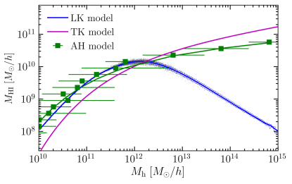
To test the model dependence of HI bias, we also assign the HI mass inside a halo by using the average HI-halo mass relation obtained from two other approaches. One approach uses the IllustrisTNG simulation (their gas data)(Villaescusa-Navarro et al., 2018) and the same star formation model(Krumholz et al., 2008, 2009a, 2009b; Krumholz, 2013). This model is dubbed “TK model” herein, which stands for “IllustrisTNG + Krumholz et al. model”. The average HI-halo mass relation in the other approach was obtained by using the updated measurements of ALFALFA survey and HOD model (Guo et al., 2017) (only available at $z=0$), and this model is dubbed “AH model”, which stands for “ALFALFA data + HOD model”. Following the fitting formula of average HI-halo mass relation in Villaescusa-Navarro et al. (2018), we use the following expression for both TK and AH models,

$$M_{\mathrm{HI}}(M_{\rm h},z)=M_{0}\left(\frac{M_{\rm h}}{M_{\min}}\right)^{\alpha}\exp\left[-\left(\frac{M_{\min}}{M_{\rm h}}\right)^{0.35}\right]\,.$$ (4)

The bestfit parameter values, as listed in Table 1, are taken from Villaescusa-Navarro et al. (2018) (their Table 1 for FoF halos) for the TK model, and obtained by $\chi^{2}$-fitting the $M_{\rm HI}$-$M_{h}$ data at $z=0$ for the AH model.

Table 1: Parameter values used for the TK and AH models.

Model	$z$	$\alpha$	$M_{0}[M_{\odot}/h]$	$M_{\min}[M_{\odot}/h]$
TK	0	0.24	$4.3\times 10^{10}$	$2.0\times 10^{12}$
	1	0.53	$1.5\times 10^{10}$	$6.0\times 10^{11}$
	2	0.60	$1.3\times 10^{10}$	$3.6\times 10^{11}$
	3	0.76	$2.9\times 10^{9}$	$6.7\times 10^{10}$
AH	0	0.12	$2.6\times 10^{10}$	$6.9\times 10^{11}$

In Figure 1, we show the HI-halo mass relation for central galaxies at $z=0$. Our results (LK model) are compared with predictions from the IllustrisTNG simulation (TK model), and the results from updated ALFALFA observations (AH model). All results agree well for low-mass halos ($M_{\rm h}<10^{11}h^{-1}\,M_{\odot}$). We checked that this agreement holds well at higher redshifts ($0<z<2$) between LK and TK models. For massive halos, nevertheless, our model underestimates the HI mass, for two possible reasons. First, the HI mass in the TK model includes the contributions from both central and satellite galaxies, while both our model and the AH model only consider those from the central galaxies. Secondly, our empirical model might underestimate the SFR for massive halos. However, the contribution of HI gas from massive halos is generally not important due to the sharp decrease of the halo mass function towards the massive end. In addition, the slope of HI-halo mass curve declines at the high mass end, which further suppresses the contribution of HI gas inside the massive halos. We will further discuss the impact of HI modelling in the high-mass end on the linear HI bias in Section 3.2 below.

2.5 HI Power spectrum

The HI mass in each halo is smoothed onto a uniform grid with $1024^{3}$ cells, and we compute the HI power spectrum from the FFT. We only keep the power spectrum for wavenumber less than a quarter of Nyquist number ($k<1.57h\,{\rm Mpc}^{-1}$) to avoid the alias effect. In Fourier space, we can define a scale-dependent effective bias, $b_{\rm HI}(k)$,

$$\delta_{\rm HI}(\bm{k})=b_{\rm HI}(k)\,\delta_{\rm m}(\bm{k})+\epsilon(\bm{k})\,,$$ (5)

where $\epsilon({\bm{k}})$ is a stochastic component which does not correlate with the density field, $\delta_{\rm m}$. On large scales, we expect $b_{\rm HI}$ is a scale-independent linear bias.

The HI bias can be estimated using the auto-power spectrum of HI gas, $b^{\rm uncorr}_{\rm HI,auto}(k)=[P_{\rm HI}(k)/P_{\rm{m}}(k)]^{1/2}$, if the shot noise is uncorrected. The leading-order mass-weighted HI shot noise is estimated by shuffling HI gas randomly, i.e. $P_{\rm SN}=V_{\rm survey}^{-1}\langle\epsilon({\bm{k}})\epsilon(-{\bm{k}})\rangle$, and then subtracted from the raw power spectrum. After correcting for shot noise, we have

$$b_{\rm HI,auto}(k)=\sqrt{\frac{P_{\rm HI}(k)-P_{\rm SN}}{P_{\rm m}(k)}}\,.$$ (6)

The assumption of HI linearity can be tested by checking if the HI bias, $b_{\rm HI,auto}(k)$, is equal to the scale-independent linear bias at large scales. Of course, the HI bias is expected to be scale-dependent at small scales due to nonlinear evolution.

The HI bias may also be estimated using the cross-power spectrum between HI density and total matter density,

$$b_{\rm HI,cross}(k)=\frac{P_{\rm HI,m}(k)}{P_{\rm m}(k)}.$$ (7)

This estimator avoids the shot noise automatically. However, in this paper, we choose to estimate the HI bias based on the auto-power spectrum of HI gas, because the 21 cm intensity mapping measures the auto-power spectrum of the 21 cm brightness temperature. As shown below in Section 3.3, the results from these two estimators are in good agreement. Thus we neglect the subscript “auto” throughout this paper except in Section 3.3.

Figure 2: The bias of halo mass density fluctuations (red) and HI mass density fluctuations derived from the LK(blue), TK(magenta), and AH(green) models at $z=0$, 1, 2, and 3, respectively, with respect to the matter density fluctuations, with shot-noised corrected (thick solid lines) and uncorrected (thin solid lines). The dashed lines indicate the constant linear bias which is estimated by averaging over $k=0.025$ — 0.075 $h\,{\rm Mpc}^{-1}$ (we neglect the smallest $k$-mode due to its relatively large cosmic variance). The dot-dashed vertical lines mark the wavenumbers of the first (black) and second (grey) BAO peaks.

3 Results and Discussion

3.1 Generic behavior

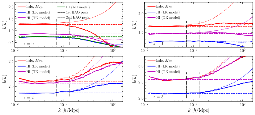
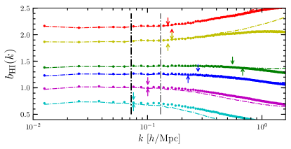
In Figure 2, we show the HI bias from different HI-halo mass relations at different redshifts (except that the AH model is only at $z=0$) as well as the halo bias. In all three models, the HI bias remains a constant at large scales for $k\lesssim 0.1\,h\,{\rm Mpc}^{-1}$, i.e. we confirm that, generically, HI gas is indeed a linear biased tracer at the first BAO peak. However, the linearity assumption begins to break down at the second BAO peak. To test whether this break-down scale relies on the halo resolution in our simulation, we vary the minimum halo mass from $10^{10}h^{-1}\,M_{\odot}$ to $10^{11}h^{-1}\,M_{\odot}$, and find that while the amplitude of HI bias depends on the halo mass cutoff similar to that of the halo bias, the linearity break-down scale is almost unchanged. Also, to test the effect of satellite galaxies, we estimate the HI masses from satellite galaxies and assign them to the centers of subhalos, using the LK model at $z=0$. We find that including satellites does not change the shape of the HI power spectrum significantly on scales $k\lesssim 1\,h\,{\rm Mpc}^{-1}$.

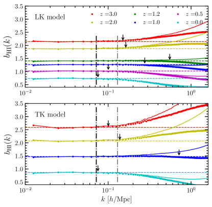
The behaviors at small scales are more interesting, as most of the HI gas resides only inside halos after cosmic reionization. Figure 2 shows that nonlinear halo clustering always enhances the halo power spectrum at small scales (before corrected for shot noise). However, Figure 1 shows that HI mass is suppressed in large halos. This suppression decreases the HI density fluctuations at small scales relative to the level of fluctuations caused by halos (see Fig.  2). The HI suppression effect is stronger at lower redshifts as more massive halos form. The competition between these two opposite effects, namely the nonlinear effects in halo clustering and those modulating the HI gas in halos, determines the evolution of the HI bias at small scales. As shown in Figure 3, for both LK and TK models, the HI bias at small scales is enhanced with respect to the linear bias at high redshifts, just like the nonlinear halo bias, while the HI bias is actually suppressed at small scales at $z=0$.

The halo bias is known to become scale-dependent at $k\gtrsim 0.1\,h\,{\rm Mpc}^{-1}$ (Jeong & Komatsu, 2009; Nishizawa et al., 2013) from N-body simulations. Naively, this sets the generic scale for the breakdown of linearity in HI bias, since most of the HI gas resides inside halos after cosmic reionization. Nevertheless, the nonlinearity of the HI content significantly affects the level of HI fluctuations with respect to halo biasing, thereby modulating the breakdown scale and making it redshift-dependent, as shown in Figure 3. In particular, these two nonlinear effects appear to balance each other at a transition time where the HI bias is linear down to small scales. In the LK model, this “sweet-spot” redshift is near $z=1.2$, with the linearity extending down to a scale $k\simeq 0.5\,h\,{\rm Mpc}^{-1}$. In the TK model, the transition takes place at $z\approx 1$, with the linearity extending down to $k\simeq 0.7\,h\,{\rm Mpc}^{-1}$. Thus, the “sweet-spot” redshift is likely to be near $z=1$, although the exact value is model-dependent.

Figure 3: The redshift evolution of the HI bias from $z=0$ to $3$, from the LK model (top) and the TK model (bottom), with shot-noised corrected (thick solid lines) and uncorrected (thin solid lines). The dashed lines indicate the constant linear bias which is estimated by averaging over $k=0.025$ — 0.075 $h\,{\rm Mpc}^{-1}$. The arrow marks the scale at which the HI bias deviates from the linear bias at the 1.5% level. The dot-dashed vertical lines mark the scales of the first (black) and second (grey) BAO peaks.

Figure 4: The redshift evolution of the HI linear bias in the LK model (blue dots) and the TK model (magenta dots). We fit the data linearly between $z=1$ and 2 (dot-dashed lines). For diagnostic purpose, we plot the prediction of linear HI bias if HI density power spectra at different redshifts would be the same as in $z=1$ but matter density fluctuations evolve according to linear theory (dashed lines). We also plot the ratio $P_{\rm HI}(k,z)/P_{\rm HI}(k,z=1)$ for both models in insets.

Figure 5: The contribution to the linear HI bias from different logarithmic halo mass bin for the LK (blue), TK (magenta), and AH (green) model at $z=0$.

3.2 Linear HI bias

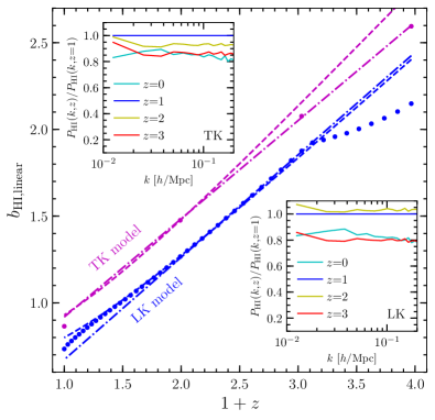
The linear HI bias (i.e. the constant HI bias averaged over large scales) increases with redshift, as shown in Figure 4. We find an interesting feature in both LK and TK models. In general, the HI bias varies approximately linearly with redshift. This linear relation is almost exact between $z=1$ and 2, with an error $<10\%$ for $z<1$ and $<15\%$ for $2<z<3$. This can be understood as follows. The linear HI bias can be written as $b_{\rm HI,linear}(z)=\big{[}D_{\rm HI}(z)/D_{\rm m}(z)\big{]}\,b_{\rm HI,linear}(1)$, where $D_{\rm HI}$ and $D_{\rm m}$ are the linear growth functions of the HI and matter density fluctuations, respectively, i.e. $D_{\rm HI}(z)=\big{[}P_{\rm HI}(z)/P_{\rm HI}(1)\big{]}^{1/2}$ and $D_{\rm m}(z)=\big{[}P_{\rm m}(z)/P_{\rm m}(1)\big{]}^{1/2}$. As shown in the insets of Figure 4, the HI density power spectrum varies only slightly with redshift, i.e. $D_{\rm HI}(z)\approx 1$. The similar result was also found in Villaescusa-Navarro et al. (2018). The reason that HI clustering only weakly varies at $0<z<3$ is an interesting open question. On the other hand, in a matter-dominated universe, the matter growth function scales as $D_{\rm m}(z)\propto(1+z)^{-1}$ (Cooray & Sheth, 2002). These two effects combined lead to the linear scaling relation, $b_{\rm HI,linear}(z)\propto(1+z)$, which we find to be generic. There are two reasons why this relation is not exactly linear. First, $D_{\rm m}(z)$ is suppressed at $z<1$ when dark energy kicks in. Secondly, the HI power spectrum has small, non-monotonous, evolution with redshift. As an illustration, consider a case in which $D_{\rm HI}(z)=1$, but $D_{\rm m}(z)$ takes the value from the linear perturbation theory (including the effect of dark energy). We find that the prediction of the linear HI bias in this case agrees with the actual results in both models, with $<15\%$ error. This is consistent with the fact that the HI power spectrum reaches its maximum at $z\simeq 1-2$, with the values at $z=0$ and $3$ about 20% lower than the maximum.

Other than the generic results presented above, however, the value of the linear HI bias can be model-dependent. Figures 2–4 show that in general the TK model predicts a higher value of linear HI bias than the LK and AH models. This difference might be attributed to the contributions of the HI gas in massive halos. We can understand this with halo model, in which the linear bias can be written as the integration of contributions from halos with different mass,

$$b_{\mathrm{HI,linear}}(z)=\frac{\int_{M_{\rm min}}^{M_{\rm max}}n(M_{\rm h},z)\,b(M_{\rm h},z)\,M_{\mathrm{HI}}(M_{\rm h},z)\,dM_{\rm h}}{\int_{M_{\rm min}}^{M_{\rm max}}n(M_{\rm h},z)\,M_{\mathrm{HI}}(M_{\rm h},z)\,dM_{\rm h}}.$$

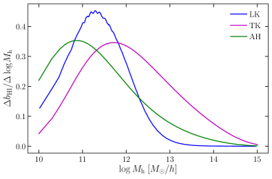
We calculate the prediction of linear HI bias in halo model using the fitting formula of the halo bias $b(M_{\rm h},z)$ and halo abundance $n(M_{\rm h},z)$ in Tinker et al. (2008, 2010), and the average HI-halo mass relation for all three models at $z=0$, and find the results agree quite well with the bias directly measured from the simulation. In Fig. 5, we show the contribution to the HI bias from each logarithmic halo mass bin of finite stepsize,

$$\frac{\Delta b_{\rm HI}(M_{\rm h})}{\Delta\log M_{\rm h}}=\frac{n(M_{\rm h},z)b(M_{\rm h},z)M_{\mathrm{HI}}(M_{\rm h},z)\left(\Delta M_{\rm h}/\Delta\log M_{\rm h}\right)}{\int_{M_{\rm min}}^{M_{\rm max}}n(M_{\rm h},z)M_{\mathrm{HI}}(M_{\rm h},z){\rm d}M_{\rm h}}.$$

(For the $n^{\rm th}$-bin, $\Delta M=M_{n+1}-M_{n}$, $\Delta\log M=\log M_{n+1}-\log M_{n}$.) For all three models, Fig. 5 shows that the peak contribution appears at $M_{\rm h}=10^{11}-10^{12}\,M_{\odot}/h$, i.e. the intermediate-mass halos contribute most to the linear HI bias. If we add up the contributions from different halo mass bins, we find that the massive halos of $M_{\rm h}=10^{14}-10^{15}\,M_{\odot}/h$ only contribute to $3.7\%$ of the linear HI bias in TK model, but contribute to about $30\%$ of the linear halo bias. This indicates that the decreasing slope of the HI-halo mass relation at the high mass end indeed further suppresses the linear HI bias. Since the HI mass is more suppressed in the massive halos in the LK and AH model than in the TK model, this explains why the linear HI bias is smaller in the former. We also point out that since the contribution at our lower mass limit $M_{\rm h}=10^{10}M_{\odot}/h$ does not vanish in Fig. 5, especially for the LK and AH model, our results of linear HI bias may be overestimated due to the neglect of unresolved smaller-mass halos which smooth out the fluctuations.

Figure 6: The HI bias defined by auto-power spectrum after correcting for shot noise, $b_{\rm HI,auto}$ (dots) (see equation 6), and cross-power spectrum, $b_{\rm HI,cross}$ (dot-dashed lines) (see equation 7), at various redshifts $z=3.0$, 2.0, 1.2, 1.0, 0.5, and 0 (for dots and lines from top to bottom, respectively) in the LK model. The upward and downward arrows mark the scale at which the HI bias $b_{\rm HI,cross}$ and $b_{\rm HI,auto}$ deviate from the linear bias at the 1.5% level, respectively.

3.3 Auto- vs. cross-power spectrum

In Figure 6, we compare the HI bias obtained from the auto-power spectrum with that obtained from the cross-power spectrum. The two results agree very well with each other down to very small scales. We note that the small difference between them does not affect any of the conclusions reached above.

3.4 Comparison with previous work

Pénin et al. (2018) performed an analytical calculation that accounts for the contribution from nonlinear matter fluctuations and nonlinear HI modulation, using the combination of a perturbation theory and a halo model. They employed six different fitting formulae for the HI-halo mass relation at $z=1$. Their results show that the HI bias is scale-independent in the range $k=0.01-0.1\,h\,{\rm Mpc}^{-1}$. However, their results indicate that the HI bias is weakly scale-dependent at $k\sim 0.001\,h\,{\rm Mpc}^{-1}$ and significantly scale-dependent at $k>0.1\,h\,{\rm Mpc}^{-1}$ (see their figure 4), which is different from our results. Because of the limitation of our simulation volume, our results are reliable only for $k>0.01\,h\,{\rm Mpc}^{-1}$, which makes it difficult to test the presence of scale-dependence on ultra-large scales. The redshift $z=1$ in our results is near the sweet-spot redshift where the HI bias is scale-independent down to scales smaller than $k\sim 0.1\,h\,{\rm Mpc}^{-1}$. The difference on small scales may be due to the different methodologies adopted in the two investigations. While perturbative calculations can provide important insights, numerical simulations can account for nonlinear effects more accurately.

Umeh et al. (2016) and Pénin et al. (2018) investigated nonlinear effects in observations, such as nonlinear redshift-space distortion and nonlinear lensing, based on perturbative calculations, and found that these nonlinearities can also produce scale-dependent bias on large scales. We will explore these effects in numerical simulations in the future.

Spinelli et al. (2020) investigated the HI content in halos using N-body simulations and semi-analytical model of galaxy evolution and gas content. This approach is similar to ours but the two differ in details. Their simulation box is the same as ours, both in a comoving volume of $500\,h^{-1}\,{\rm Mpc}$ on each side. They found that the HI bias is scale-independent on large scales, which is similar to ours, but their results are much noisier (see their Figure 12). They also found that the HI bias is enhanced at high redshifts. However, the HI bias in their results is roughly scale-independent down to $k\sim 2\,h\,{\rm Mpc}^{-1}$ up to $z=2$. In contrast, our results show that the small-scale bias evolves from being enhanced at higher redshift to being suppressed at $z<1$, and that there is a sweet-spot redshift near $z=1$. This difference is likely due to different treatments in the HI contents of halos, which can lead to different suppression of the nonlinear HI modulation.

Villaescusa-Navarro et al. (2018) made a comprehensive analysis of HI gas distribution based on the IllustrisTNG megneto-hydrodynamic simulation. They employed the similar gas model (Krumholz et al., 2008, 2009a, 2009b; Krumholz, 2013) to ours, to divide the cold hydrogen gas within each cell into atomic and molecular components. Due to the limited simulation volume ($\sim 100\,h^{-1}\,{\rm Mpc}$ on each side), Villaescusa-Navarro et al. (2018) cannot test the scale-dependence of the HI bias at the first BAO peak scale. In comparison, our work applied the average HI-halo mass relation from Villaescusa-Navarro et al. (2018), nevertheless, to halos resolved from our N-body simulation with large enough volume ($500\,h^{-1}\,{\rm Mpc}$ on each side) — i.e. our TK model — to avoid the finite box effect on the bias at the BAO scales. Therefore, we can directly confirm from simulation that the HI bias is linear at the scale corresponding to the first BAO peak. On the other hand, both Villaescusa-Navarro et al. (2018) and our work find that the HI bias linearity becomes to break down at $k\gtrsim 0.1h\,{\rm Mpc}^{-1}$ generically, the smallest wavenumber presented in Villaescusa-Navarro et al. (2018).

Modi et al. (2019) investigated the clustering of HI gas using the Hidden Valley N-body simulation which has a large comoving volume of 1 $h^{-1}\,{\rm Gpc}$ on each side at $z=2-6$, so their work is complementary to ours regarding the focused regime of redshift. The Hidden Valley simulation can resolve halos down to $10^{9}M_{\odot}/h$, so they can incorporate the HI gas inside smaller-mass halos at high redshifts than our work. They adopted fitting formulae of average HI-halo mass relation similar to Eq. (4) herein, in order to assign HI mass to halos, and explore both two-point correlation function and power spectrum. Similar to our results, they also found that the HI bias becomes scale-dependent at $k\gtrsim 0.1h\,{\rm Mpc}^{-1}$. Their results indicate a strong scale-dependence of HI bias at the large $k$ at the high redshift, which is consistent with the behavior in our results for the redshifts higher than the sweet-spot $z\approx 1$.

4 Summary

In this paper, we use a large N-body simulation to explore the HI bias for 21 cm intensity mapping experiments at low redshifts. We adopt three models, LK, TK and AH, representing empirically, numerically, and observationally oriented approaches, respectively, to assign HI mass to dark matter halos and to account for uncertainties in the HI-halo mass relation.

We confirm that the HI gas distribution is a linearly biased tracer of the total dark matter density field on the scales corresponding to the first BAO peak. However, the HI linearity assumption breaks down at $k>0.1\,h\,{\rm Mpc}^{-1}$. The exact breakdown scale is redshift-dependent, because the nonlinear effects that modulate the HI gas in halos evolve with time. This HI nonlinearity, which is caused by the nonlinear halo clustering and nonlinear HI content modulation, is intrinsic and not related to the instrumental and observational effects. This imposes a challenge to the upcoming 21 cm intensity mapping experiments in their capabilities to extract cosmological information from the broadband shape of the 21 cm power spectrum in this $k$-range where a large number of modes are located. The result is particularly important for forecasting cosmological constraints with upcoming 21 cm intensity mapping experiments. It is, therefore, necessary to better model the HI power spectrum beyond the linear regime, e.g. applying the large-scale structure perturbation theory at the quasi-linear scales. We note, however, that cosmological constraints from the BAO measurement of the 21 cm power spectrum is not affected by the nonlinear bias.

We find the existence of a characteristic redshift above and below which the small scale HI bias is enhanced and suppressed relative to the linear bias, respectively. For redshifts close to this “sweet spot”, the HI bias is linear down to small scales. For example, for the LK model, the characteristic redshift is $\simeq 1.2$, at which the linearity of the bias extends from large scales all the way down to $k\simeq 0.5\,h\,{\rm Mpc}^{-1}$. However, the exact value of this “sweet spot" redshift depends both on the HI-halo mass relation and on nonlinear clustering of halos. Determining the “sweet-spot" redshift observationally can, therefore, also provide valuable information on star formation and clustering of dark matter halos.

Finally, we also find that the linear HI bias is an approximately linear function of redshift for $z\leq 3$. This may make cross-checks between different redshifts more powerful for interpreting observational data.

References

- Ando et al. (2019) Ando, R., Nishizawa, A. J., Hasegawa, K., Shimizu, I., & Nagamine, K. 2019, MNRAS, 484, 5389
- Bagla et al. (2010) Bagla, J. S., Khandai, N., & Datta, K. K. 2010, MNRAS, 407, 567
- Bandura et al. (2014) Bandura, K., Addison, G. E., Amiri, M., et al. 2014, in Ground-based and Airborne Telescopes V, Vol. 9145, International Society for Optics and Photonics, 914522
- Battye (2013) Battye, R. 2013, MNRAS, 434, 1239
- Cai et al. (2016) Cai, Z., Fan, X., Peirani, S., et al. 2016, ApJ, 833, 135
- Cai et al. (2017) Cai, Z., Fan, X., Bian, F., et al. 2017, ApJ, 839, 131
- Chang et al. (2010) Chang, T.-C., Pen, U.-L., Bandura, K., & Peterson, J. B. 2010, Nature, 466, 463
- Chang et al. (2008) Chang, T.-C., Pen, U.-L., Peterson, J. B., & McDonald, P. 2008, Phys. Rev. Lett., 100, 091303
- Chen (2012) Chen, X. 2012, in International Journal of Modern Physics: Conference Series, Vol. 12, World Scientific, 256–263
- Chen et al. (2019) Chen, Y., Mo, H. J., Li, C., et al. 2019, ApJ, 872, 180
- Cooray & Sheth (2002) Cooray, A., & Sheth, R. 2002, Physics Reports, 372, 1
- Cui et al. (2017) Cui, W., Knebe, A., Yepes, G., et al. 2017, MNRAS, 473, 68
- d’Amico et al. (2020) d’Amico, G., Gleyzes, J., Kokron, N., et al. 2020, J. Cosmology Astropart. Phys, 2020, 005
- Desjacques et al. (2018) Desjacques, V., Jeong, D., & Schmidt, F. 2018, Phys. Rep., 733, 1
- Diemer et al. (2018) Diemer, B., Stevens, A. R., Forbes, J. C., et al. 2018, The Astrophysical Journal Supplement Series, 238, 33
- Dunkley et al. (2009) Dunkley, J., Komatsu, E., Nolta, M., et al. 2009, ApJS, 180, 306
- Dutton et al. (2011) Dutton, A. A., Bosch, F. C. v. d., Faber, S. M., et al. 2011, MNRAS, 410, 1660
- Fry (1996) Fry, J. N. 1996, The Astrophysical Journal, 461
- Guha Sarkar et al. (2012) Guha Sarkar, T., Mitra, S., Majumdar, S., & Choudhury, T. R. 2012, MNRAS, 421, 3570
- Guo et al. (2020) Guo, H., Jones, M. G., Haynes, M. P., & Fu, J. 2020, ApJ, 894, 92
- Guo et al. (2017) Guo, H., Li, C., Zheng, Z., et al. 2017, ApJ, 846, 61
- Jeong & Komatsu (2009) Jeong, D., & Komatsu, E. 2009, ApJ, 691, 569
- Khandai et al. (2011) Khandai, N., Sethi, S. K., Di Matteo, T., et al. 2011, MNRAS, 415, 2580
- Klypin & Prada (2019) Klypin, A., & Prada, F. 2019, MNRAS, 489, 1684
- Kravtsov (2013) Kravtsov, A. V. 2013, ApJ, 764, L31
- Krumholz (2013) Krumholz, M. R. 2013, MNRAS, 436, 2747
- Krumholz et al. (2008) Krumholz, M. R., McKee, C. F., & Tumlinson, J. 2008, ApJ, 689, 865
- Krumholz et al. (2009a) —. 2009a, ApJ, 693, 216
- Krumholz et al. (2009b) —. 2009b, ApJ, 699, 850
- Loeb & Wyithe (2008) Loeb, A., & Wyithe, J. S. B. 2008, Phys. Rev. Lett., 100, 161301
- Lu et al. (2015) Lu, Z., Mo, H., & Lu, Y. 2015, MNRAS, 450, 606
- Lu et al. (2014) Lu, Z., Mo, H., Lu, Y., et al. 2014, MNRAS, 439, 1294
- Ma et al. (2015) Ma, X., Hopkins, P. F., Faucher-Giguère, C.-A., et al. 2015, MNRAS, 456, 2140
- Modi et al. (2019) Modi, C., Castorina, E., Feng, Y., & White, M. 2019, J. Cosmology Astropart. Phys, 2019, 024
- Newburgh et al. (2016) Newburgh, L., Bandura, K., Bucher, M., et al. 2016, in Ground-based and Airborne Telescopes VI, Vol. 9906, International Society for Optics and Photonics, 99065X
- Nishizawa et al. (2013) Nishizawa, A. J., Takada, M., & Nishimichi, T. 2013, MNRAS, 433, 209
- Padmanabhan et al. (2016) Padmanabhan, H., Choudhury, T. R., & Refregier, A. 2016, MNRAS, 458, 781
- Padmanabhan & Refregier (2017) Padmanabhan, H., & Refregier, A. 2017, MNRAS, 464, 4008
- Padmanabhan et al. (2017) Padmanabhan, H., Refregier, A., & Amara, A. 2017, MNRAS, 469, 2323
- Pénin et al. (2018) Pénin, A., Umeh, O., & Santos, M. G. 2018, MNRAS, 473, 4297
- Pritchard et al. (2015) Pritchard, J., Ichiki, K., Mesinger, A., et al. 2015, in Advancing Astrophysics with the Square Kilometre Array (AASKA14), 12
- Sarkar & Bharadwaj (2018) Sarkar, D., & Bharadwaj, S. 2018, MNRAS, 476, 96
- Sarkar et al. (2016) Sarkar, D., Bharadwaj, S., & Anathpindika, S. 2016, MNRAS, 460, 4310
- Skibba et al. (2014) Skibba, R. A., Smith, M. S. M., Coil, A. L., et al. 2014, The Astrophysical Journal, 784, 128
- Spinelli et al. (2020) Spinelli, M., Zoldan, A., De Lucia, G., Xie, L., & Viel, M. 2020, MNRAS, 493, 5434
- Springel (2005) Springel, V. 2005, MNRAS, 364, 1105
- Springel et al. (2001) Springel, V., White, S. D., Tormen, G., & Kauffmann, G. 2001, MNRAS, 328, 726
- Tinker et al. (2008) Tinker, J., Kravtsov, A. V., Klypin, A., et al. 2008, The Astrophysical Journal, 688, 709
- Tinker et al. (2010) Tinker, J. L., Robertson, B. E., Kravtsov, A. V., et al. 2010, The Astrophysical Journal, 724, 878
- Umeh et al. (2016) Umeh, O., Maartens, R., & Santos, M. 2016, J. Cosmology Astropart. Phys, 2016, 061
- Villaescusa-Navarro et al. (2018) Villaescusa-Navarro, F., Genel, S., Castorina, E., et al. 2018, ApJ, 866, 135
- Wang et al. (2016) Wang, H., Mo, H., Yang, X., et al. 2016, ApJ, 831, 164
- Wyithe & Loeb (2009) Wyithe, J. S. B., & Loeb, A. 2009, MNRAS, 397, 1926