Nuclear level densities and gamma-ray strength functions of ^180,181,182Ta

Abstract

Particle-$\gamma$ coincidence experiments were performed at the Oslo Cyclotron Laboratory with the ¹⁸¹Ta(d,X) and ¹⁸¹Ta(³He,X) reactions, to measure the nuclear level densities (NLDs) and $\gamma$-ray strength functions ($\gamma$SFs) of ^180,181,182Ta using the Oslo method. The Back-shifted Fermi-Gas, Constant Temperature plus Fermi Gas, and Hartree-Fock-Bogoliubov plus Combinatorial models where used for the absolute normalisations of the experimental NLDs at the neutron separation energies. The NLDs and $\gamma$SFs are used to calculate the corresponding ¹⁸¹Ta(n,$\gamma$) cross sections and these are compared to results from other techniques. The energy region of the scissors resonance strength is investigated and from the data and comparison to prior work it is concluded that the scissors strength splits into two distinct parts. This splitting may allow for the determination of triaxiality and a $\gamma$ deformation of $14.9^{\circ}\pm 1.8^{\circ}$ was determined for ¹⁸¹Ta.

I Introduction

The $\gamma$-ray strength function ($\gamma$SF) and nuclear level density (NLD) describe the nuclear structure in the region of the quasi-continuum where the level spacing is too small to resolve and study individual levels. The $\gamma$SF characterises the average electromagnetic properties and is related to radiative decay and photo-absorption processes Chadwick et al. (2011); Bartholomew et al. . From the NLD the evolution of the number of levels with excitation energy can be investigated Guttormsen et al. (2015) and related to thermodynamic properties Moretto et al. (2015).

The $\gamma$SF and NLD are important input parameters into reaction cross section calculations in the Hauser-Feshbach statistical framework Hauser and Feshbach (1952). The Hauser-Feshbach formalism is implemented in the TALYS v1.9 reaction code Koning et al. (2008a) which can be used to calculate (n,$\gamma$) cross sections. Hence, NLD and $\gamma$SF are nuclear properties of significance to nucleosynthesis Arnould et al. (2007) and calculations have shown that relative small changes to the overall shape of the $\gamma$SF, such as a pygmy resonance, can have an order of magnitude effect on the rate of elemental formation Goriely (1998). It has been shown that measured statistical properties can reliably be used to reproduce capture cross sections that were measured using other techniques Guttormsen et al. (2017); Kheswa et al. (2017); Larsen et al. (2016), although further validations are needed across the nuclear chart. Additionally, NLD and $\gamma$SF can also be relevant to the design of existing and future nuclear power reactors, where simulations depend on such nuclear data Chadwick et al. (2011). Their importance is highlighted by the efforts which are currently underway to generate a reference database for $\gamma$SFs Dimitriou et al. (2018).

A key feature of the $\gamma$SF in well-deformed nuclei is the scissors resonance (SR). The SR is a collective magnetic dipole (M1) excitation usually found at excitation energies $E_{x}\approx$ 2-4 MeV. The SR was predicted several decades ago Suzuki and Rowe (1977); Iudice and Palumbo (1978, 1979); Iachello (1981) and first observed in ¹⁵⁶Gd a few years later Bohle et al. (1984a). A splitting of the SR in ¹⁶⁴Dy and ¹⁷⁴Yb was reported soon after Bohle et al. (1984b) and interpreted as a possible measure of nuclear triaxiality Iudice et al. (1985). Besides observations in well-deformed even-even nuclei (Heyde et al. (2010) and references therein), the SR has also been observed in less deformed nuclei, e.g. in vibrational even-mass ^122-130Te Schwengner et al. (1997), transitional ^190,192Os Fransen et al. (1999), and in $\gamma$-soft ¹³⁴Ba and ¹⁹⁶Pt Maser et al. (1996); von Brentano et al. (1996) nuclei. The SR has been investigated through nuclear resonance fluorescence (NRF) Kneissl et al. (1996), resonance neutron capture Baramsai (2015), and through the Oslo Method in the rare-earth Schiller et al. (2000) and actinide Guttormsen et al. (2012, 2014); Tornyi et al. (2014); Laplace et al. (2016) regions. A review of the theoretical and experimental findings can be found in Ref. Heyde et al. (2010).

In this paper we present results of the NLDs and $\gamma$SFs for ^180,181,182Ta from six reactions. Three different level density models are used and compared for the normalisation at $S_{n}$. From the (d,p)¹⁸²Ta data the ¹⁸¹Ta(n,$\gamma$) cross section is calculated using TALYS and compared to previous results. The emergence of the SR in the transitional nucleus ¹⁸¹Ta is investigated and compared to other work. The paper is structured as follows: in Sec. II the experimental setup is presented and Sec. III provides a brief overview of the Oslo method and the different level density models that were used. Sec. IV presents the ¹⁸¹Ta(n,$\gamma$) cross section and a comparison to other work, while Sec. V investigates and discusses the presence of the SR in ¹⁸¹Ta. A brief summary is given in Sec. VI.

II Experimental Setup

Three experiments were performed at the Oslo Cyclotron Laboratory (OCL) at the University of Oslo using a self-supporting 0.8 mg/cm² thick natural tantalum target. A deuteron beam of 12.5 MeV was used for the ¹⁸¹Ta(d,p)¹⁸²Ta and ¹⁸¹Ta(d,d’)¹⁸¹Ta reactions, while a deuteron beam of 15 MeV was used for the ¹⁸¹Ta(d,t)¹⁸⁰Ta reaction and a second ¹⁸¹Ta(d,d’)¹⁸¹Ta reaction. A 34 MeV ³He beam was utilised for the ¹⁸¹Ta(³He,³He’)¹⁸¹Ta and ¹⁸¹Ta(³He,$\alpha$)¹⁸⁰Ta reaction. The SiRi particle telescope Guttormsen et al. (2011) and CACTUS scintillator Guttormsen et al. (1990) array were used to detect charged particles and $\gamma$-rays in coincidence within a 2$\mu$s hardware time window.

The $\Delta$E-E SiRi particle-telescope consists of eight 130 $\mu$m thin, segmented silicon $\Delta$E detectors and eight 1550 $\mu$m thick E silicon detectors. These detectors covered a polar angular range of $\theta_{lab}=126^{\circ}-140^{\circ}$ with respect to the beam axis. The energy resolutions, as determined from the elastic peaks, are $\approx$ 125 keV for the deuteron and 350 keV for the ³He beams. The CACTUS array consists of 26 NaI(Tl) detectors with $5"\times 5"$ crystals positioned 22 cm away from the target, covering a solid angle of 16.2$\%$ of $4\pi$ sr. CACTUS has a total efficiency of 14.1(1)$\%$ and an energy resolution of 6$\%$ FWHM for a 1332 keV $\gamma$-ray transition.

The E detectors provided the start signal and the delayed NaI(Tl) detectors provided the stop signal for the time-to-digital converters, enabling event-by-event sorting for the particle-$\gamma$ coincidence data. Calibrations of SiRi was accomplished using individual reactions on ¹⁸¹Ta. CACTUS detectors was calibrated with the ²⁸Si(d,p) reaction which provided appropriate $\gamma$-ray energies. During offline analysis the prompt time gate was set to 40 ns for the data sets from ³He beams and to 30 ns for the data from deuteron beams. Equivalently wide non-prompt time gates were used to subtract and remove the uncorrelated events from the prompt particle-$\gamma$ events.

III Analysis

III.1 Oslo Method

The $\gamma$SFs and NLDs are simultaneously extracted using the Oslo Method, which has been covered in the literature Schiller et al. (2000); Larsen et al. (2011); Guttormsen et al. (1996, 1987), and only a brief overview will be presented here. In the first step the $\gamma$-ray spectra is unfolded using the detector response function. The Compton background, effects from pair production and the single- and double-escape peaks are removed from the $\gamma$-ray spectrum leaving only full-energy deposit events that are corrected for efficiency. The primary $\gamma$-rays are extracted using an iterative subtraction method that separates the primary $\gamma$-rays from the total $\gamma$-ray cascade. The primary transitions are collected in the first-generation matrix $P(E_{x},E_{\gamma})$ with the assumption that the $\gamma$-ray distribution is the same for a state populated through $\gamma$-ray decay or the nuclear reaction. This assumption is valid at high-level densities where the nucleus is in a compound state prior to $\gamma$-ray emission.

The probability for a $\gamma$-ray, with energy $E_{\gamma}$, to decay from excitation energy $E_{x}$ to a final energy $E_{f}$, with energy $E_{f}=E_{x}-E_{\gamma}$, is proportional to the level density at the final energy, $\rho(E_{f})$ and the transmission coefficient $\mathcal{T}(E_{\gamma})$. $P(E_{x},E_{\gamma})$ is proportional to the decay probability and can be factorised as:

$$P(E_{x},E_{\gamma})\propto\mathcal{T}(E_{\gamma})\rho(E_{f}).$$ (1)

Brink’s hypothesis Brink (1955) is assumed to be valid, which implies that the $\gamma$-ray transmission coefficient does not depend on the properties of the initial and final states but only on the $\gamma$-ray energy. A $\chi^{2}$ minimisation is used to extract $\mathcal{T}(E_{\gamma})$ and $\rho(E_{f})$ Schiller et al. (2000):

$$\begin{split}\chi^{2}=\frac{1}{N_{free}}\sum^{E^{max}}_{E_{x}=E^{min}}\sum^{E_{x}}_{E_{\gamma}=E^{min}_{\gamma}}\times\\ \left(\frac{P_{th}(E_{x},E_{\gamma})-P(E_{x},E_{\gamma})}{\delta P(E_{x},E_{\gamma})}\right)^{2},\end{split}$$ (2)

where $N_{free}$ is the number of degrees of freedom and $\delta P(E_{x},E_{\gamma})$ is the uncertainty in the first-generation matrix. The experimental $P(E_{x},E_{\gamma})$ and fitted $P_{th}(E_{x},E_{\gamma})$ first-generation matrices for ¹⁸²Ta are shown in Fig. 1

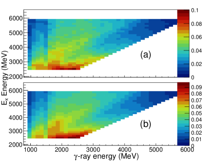
Figure 1: (Color online) The experimental (a) and fitted (b) first-generation particle-$\gamma$ matrices from the ¹⁸¹Ta(d,p)¹⁸²Ta reaction with a deuteron energy of 12.5 MeV.

. Their close similarity encourages an accurate fit. The $\chi^{2}$ minimisation was applied in the regions shown in Tab. 1.

Table 1: The regions where the $\chi^{2}$ minimisation was applied to data from the different reactions populating ^180,181,182Ta.

Reaction	Ebeam	E${}_{\gamma}^{min}$	E${}_{x}^{min}$	E${}_{x}^{max}$
	(MeV)	(MeV)	(MeV)	(MeV)
(3He,$\alpha$)180Ta	34	1.73	2.97	6.35
(3He,3He’)181Ta	34	1.63	2.57	7.38
(d,t)180Ta	15	1.21	2.49	5.18
(d,d’)181Ta	15	1.21	3.01	6.02
(d,d’)181Ta	12.5	1.59	2.54	3.84
(d,p)182Ta	12.5	1.54	2.54	5.94

Within these limits an infinite number of solutions for $P(E,E_{\gamma})$ can be found of the form:

$$\tilde{\rho}(E_{f})=Ae^{\alpha E_{f}}\rho(E_{f})$$ (3)

and

$$\widetilde{\mathcal{T}}(E_{\gamma})=Be^{\alpha E_{\gamma}}\mathcal{T}(E_{\gamma}),$$ (4)

where $A$ and $B$ are normalisation parameters and $\alpha$ is the slope of the NLD and $\gamma$-ray transmission coefficient.

III.2 Nuclear level density

A normalisation is performed to determine the parameters $A$ and $B$ and the slope $\alpha$, corresponding to the physical solutions, from other experimental data as well as systematics. The NLD is normalised at low energies to experimentally measured levels by counting the levels from the evaluated nuclear data base Brookhaven National Laboratory . At high $E_{x}$ the NLD is normalised to the total level density at the neutron separation energy $\rho(S_{n})$.

The functional form of the NLD is uniquely defined from the $\chi^{2}$ fit of the primary $\gamma$-ray matrix. It is for the absolute normalisation at the neutron separation energy that different level density models, in particular the spin distribution, play a major role. For this work three different normalisation models are considered. The Back-shifted Fermi-Gas (BSFG) Gilbert and Cameron (1965), Constant Temperature+Fermi Gas (CT+FG) Koning and Rochman (2012), and Hartree-Fock-Bogoliubov plus Combinatorial (HFB) Goriely et al. (2008).

The CT+FG normalisation is based on two different spin cut-off formulas. Firstly, using the energy-dependent spin cut-off parameter, the NLD can accurately be obtained from the widely used Constant Temperature model (CT) Gilbert and Cameron (1965), for 2$\Delta_{0}\leq E_{x}\leq$10 MeV, where $\Delta_{0}$ is the pair-gap parameter Bohr and Mottelson (1969). The total NLD $\rho(S_{n})$ is calculated according to Larsen et al. (2011):

$$\rho(S_{n})=\frac{2\sigma^{2}}{D_{0}}\times\frac{1}{(I+1)\text{exp}(-\frac{(I+1)^{2}}{2\sigma^{2}})+I\text{exp}(-\frac{I^{2}}{2\sigma^{2}})}.$$ (5)

$D_{0}$ is the $\ell=0$ neutron resonance spacing data Capote et al. (2009); Mughabghab (2006), $I$ is the initial spin of the target nucleus, and the spin cut-off parameter $\sigma$ is determined from von Egidy and Bucurescu (2009):

$$\sigma^{2}=0.391A^{0.675}(E_{x}-0.5Pa)^{0.312}$$ (6)

where $A$ is the number of nucleons and $Pa$ is the deuteron pairing energy. When using this spin distribution the model will be referred to as CT+FG1. Since the NLD can only be extracted up to $E_{x}-E_{\gamma}$ and does not reach $S_{n}$, the CT model Koning et al. (2008b) is used to interpolate between the experimental NLD and $\rho(S_{n})$. The experimentally extracted ¹⁸¹Ta NLD with CT+FG1 from all three reactions populating ¹⁸¹Ta are shown in Fig. 2

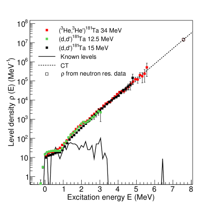
Figure 2: (Color online) The NLDs of ¹⁸¹Ta from the 12.5 MeV ¹⁸¹Ta(d,d’) (green), 15 MeV ¹⁸¹Ta(d,d’) (black) and ¹⁸¹Ta(³He,³He’) (red) reactions using the CT+FG1 model. The solid line represents the level density deduced from known levels. The dashed line from the CT model Koning et al. (2008b), interpolates between the experimental data and $\rho(S_{n})$ (black open square).

and are in good agreement. Secondly, the CT+FG normalisation uses the spin cut-off parameter as implemented in TALYS Koning et al. (2008a). The $E_{x}$ is divided into two excitation energy regions: 0 $\leq$$E_{x}$ $\leq$ $E_{M}$, where the constant temperature approximation applies and $E_{x}>E_{M}$, where the Fermi-gas model applies Ericson (1959). $E_{M}$ is the matching excitation energy between the two models. When using the spin distribution from TALYS the model will be referred to as CT+FG2.

The microscopic HFB model describes the energy-, spin- and parity-dependent NLD. This model takes into account the HFB single-particle level scheme to calculate incoherent intrinsic state densities which depends only on $E_{x}$, parity and the spin projection on the symmetry axis of the nucleus. The collective (rotational and vibrational) enhancement are accounted for, once the incoherent particle-hole states densities have been determined. The resulting microscopic approach reproduces well the experimental data at known discrete states and $S_{n}$. These NLDs are tabulated in the TALYS software package.

The BSFG model Gilbert and Cameron (1965); Dilg et al. (1973) for the NLD is based on the Fermi-gas approximation and includes pairing energies and shell correction effects in its calculations. In this model the level density parameter and energy shift are free parameters to allow for a reasonable fit to experimental data.

In the case of ¹⁸⁰Ta, neither $D_{0}$ nor the average radiative width, $\langle\mathit{\Gamma_{\gamma 0}}\rangle$ are known. The $\rho(S_{n})$ was estimated by normalising both $\rho(E_{x})$ and $\mathcal{T}(E_{\gamma})$ of ¹⁸⁰Ta on the basis of these functions having the same slope as $\rho(E_{x})$ and $\mathcal{T}(E_{\gamma})$ of ^181,182Ta using eqn. 5. It has been shown that $\rho(E_{x})$ and $\mathcal{T}(E_{\gamma})$ of neighbouring isotopes have the same slope Moretto et al. (2015), independent of the normalisation method used. The spline fit function, as implemented in TALYS Koning et al. (2008a), was used to estimate $\langle\mathit{\Gamma_{\gamma 0}}\rangle$.

The NLDs of ^180,181,182Ta using the three normalisations are shown in Fig. 3

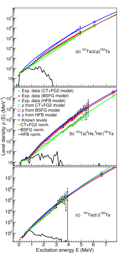
Figure 3: (Color online) The NLD of ¹⁸²Ta from the (d,p) reaction (a), ¹⁸¹Ta from the (³He,³He’) reaction (b), and ¹⁸⁰Ta from the (d,t) reaction (c) are shown with CT+FG2, BSFG and HFB normalisations (see text for details).

. The open squares are the $\rho(S_{n})$ and the solid lines are the level density calculated by the individual models. The experimental data are then normalised to these calculations and are superimposed for comparison. All the models reproduced the $D_{0}$ within experimental uncertainties. The different models will be used later to constrain the upper and lower uncertainties for the cross section calculations. The NLD of the odd-odd ^180,182Ta are higher than that of the even-odd ¹⁸¹Ta, due to one extra unpaired neutron in ^180,182Ta which increases the number of degrees of freedom.

III.3 $\gamma$-ray strength function

Assuming that the statistical $\gamma$-ray decays are dominated by dipole transitions the $\gamma$SF is given by Capote et al. (2009):

$$f(E_{\gamma})=\frac{\tilde{\mathcal{T}}(E_{\gamma})}{2\pi E_{\gamma}^{3}}.$$ (7)

The absolute normalisation parameter $B$ is obtained by constraining the data to $\langle\mathit{\Gamma_{\gamma 0}}\rangle$ for s-wave resonances by Kopecky and Uhl (1990):

$$\begin{split}&\langle\varGamma_{\gamma 0}(S_{n})\rangle=\frac{1}{2\pi\rho(S_{n},I_{T},\pi_{T})}\sum_{I_{f}}\int_{0}^{S_{n}}\times\\ &B\mathcal{T}(E_{\gamma})\rho(S_{n}-E_{\gamma},I_{f})dE_{\gamma},\\ \end{split}$$ (8)

where $\pi$ is the parity, the subscripts $f$ and $T$ indicate the final levels and target nucleus, respectively.

The photo absorption cross section, $\sigma(E_{\gamma})$, can be converted to the $\gamma$SF by Bartholomew et al. :

$$f(E_{\gamma})=\frac{\sigma(E_{\gamma})}{3E_{\gamma}(\pi\hbar c)^{2}}.$$ (9)

The extracted $\gamma$SFs for ^180,181,182Ta are shown for each reaction individually in Fig. 4

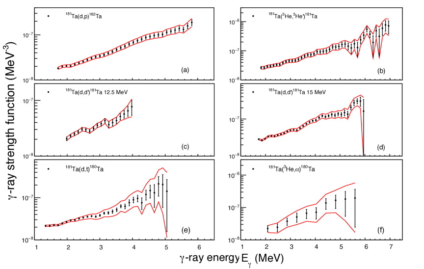
Figure 4: (Color online) The $\gamma$SFs for ^180,181,182Ta for each reaction are shown as black circles with the systematic and statistical uncertainties represented by the error bars. The red lines are the extent of the upper and lower uncertainties which include the experimental uncertainties in $D_{0}$ and $\langle\mathit{\Gamma_{\gamma 0}}\rangle$, in addition to systematic and statistical uncertainties.

. For ¹⁸²Ta (Fig. 4 (a)) the $\gamma$SF is relatively smooth in the measured range with a possible slight enhancement at $\sim$4.5 MeV which has been reported previously in Igashira et al. (1986). The $\gamma$SFs for ¹⁸¹Ta exhibit some features which will be discussed in Sec. V. The $\gamma$SF from the ¹⁸⁰Ta(³He,$\alpha$) reaction had low statistics resulting in larger binning and uncertainties. The uncertainties of the $\gamma$SF normalisation introduced by $D_{0}$ and $\langle\mathit{\Gamma_{\gamma 0}}\rangle$ from Refs. Capote et al. (2009); Mughabghab (2006) were considered by separately extracting upper and lower NLDs and $\gamma$SFs for the experimental data, using $D_{0}=D_{0}\mp\delta D_{0}$ and $\langle\mathit{\Gamma_{\gamma 0}}\rangle\;=\;\langle\mathit{\Gamma_{\gamma 0}}\rangle\pm\langle\delta\mathit{\Gamma_{\gamma 0}}\rangle$ with the CT+FG1. This produces upper and lower error bands. The parameters used to normalise the $\gamma$SFs and NLDs are listed in Tab. 2. All $\gamma$SFs for each nucleus are plotted together, with data obtained from ¹⁸¹Ta($\gamma$,n) Utsunomiya et al. (2003), ¹⁸¹Ta($\gamma$,xn) Bergère et al. (1968) and ¹⁸¹Ta$(\gamma,\gamma)$ Makinaga et al. (2014), in Fig. 5

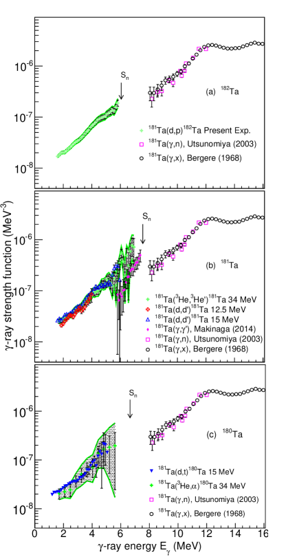
Figure 5: (Color online) The experimental $\gamma$SFs of ¹⁸²Ta (a), ¹⁸¹Ta (b) and ¹⁸⁰Ta (c) from present experiments, are compared to data obtained from ¹⁸¹Ta($\gamma$,n) Utsunomiya et al. (2003), ¹⁸¹Ta($\gamma$,xn) Bergère et al. (1968) and ¹⁸¹Ta$(\gamma,\gamma)$ Makinaga et al. (2014). The upper and lower uncertainty bands (green lines) are the combination of statistical, systematic and experimental uncertainties due to D₀ and $\langle\mathit{\Gamma_{\gamma 0}}\rangle$. Here, they are shown only for the data with the largest uncertainties.

. The $\gamma$SFs for the same nucleus obtained from different reactions are quite similar and agree within the uncertainties.

The experimental $\gamma$SF has contributions from E1 and M1 transitions, and therefore has to be disentangled. This is achieved by subtracting the $M1$ D1M-QRPA strength Goriely et al. (2016, 2018) (Quasi-Particle Random Phase Approximation based on the Gogny D1M interaction) from the experimental E1+M1 $\gamma$SF as shown in Fig. 6

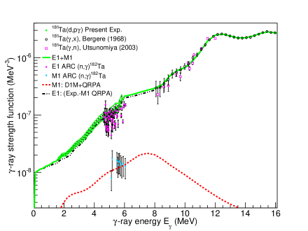
Figure 6: (Color online) The experimental $\gamma$SFs have contributions from E1 and M1 transitions and need to be disentangled. The disentangled E1 and M1 contributions for ¹⁸²Ta are compared to ARC data from Ref. Kopecky et al. (2017).

. The disentangled E1 and M1 contributions agree well with average reaction capture (ARC) data from Ref. Kopecky et al. (2017). The same procedure was applied in the analysis of ^91,92Zr isotopes Guttormsen et al. (2017). This disentanglement was performed for the experimental strengths from each data set individually.

IV ¹⁸¹Ta(n,$\gamma$) cross sections

The E1 and M1 strengths plus the ¹⁸¹Ta NLDs are used as input in TALYS. The experimental $\gamma$SF span the energy region $E_{\gamma}^{min}$ $\lesssim E_{\gamma}^{exp}\lesssim S_{n}$. The data was extrapolated for $E_{\gamma}^{min}\rightarrow 0$ and $E_{\gamma}^{exp}\rightarrow S_{n}$ to reproduce the experimental $\langle\mathit{\Gamma_{\gamma 0}}\rangle$ values within $<5\%$. Here $E_{\gamma}^{exp}$ is the present experimental data. A linear fit was used to extrapolate the data between the $\gamma$SF and the Giant Electric Dipole Resonance (GEDR) data.

Whenever possible it is prudent to benchmark existing (n,$\gamma$) cross sections to those that can be obtained using experimental NLDs and $\gamma$SFs. The ¹⁸¹Ta(n,$\gamma$) cross sections were calculated using the nuclear reactions code TALYS. The key ingredients in the calculations of these (n,$\gamma$) cross sections using the Hauser Feshbach (HF) approach are: the nuclear structure properties (i.e., masses, deformation, $E_{x}$, $J^{\pi}$, etc), NLD, $\gamma$SF and optical model potentials. The global neutron optical potential of Koning and Delaroche (2003) was used for all nuclei in discussion. The Hofmann-Richert-Tepel-Weidenmüller-model (HRTW) Hofmann et al. (1975) for width fluctuation corrections in the compound nucleus calculation was used.

Table 2: The $\gamma$SF and NLD normalisation parameters: resonance spacing $D_{0}$, average radiative width $\langle\mathit{\Gamma_{\gamma 0}}\rangle$, spin-cutoff parameter $\sigma$, level density at the neutron separation energy $\rho(S_{n})$ from the CT+FG1, level density parameter $a$, back-shifted energy $E_{1}$, and the neutron separation energy $S_{n}$.

Nucleus	$D_{0}$ (eV)	$\langle\mathit{\Gamma_{\gamma 0}}\rangle$ (meV)	$\sigma(S_{n})^{b}$	$\rho(S_{n})^{c}$ (106 MeV${}^{-1})$	$a$ (MeV-1)	$E_{1}$ (MeV)	$S_{n}$ (MeV)
180Ta	0.80 $\pm$ 0.24d	62.0 $\pm$ 5.8d	4.93 $\pm$ 0.49	10.67 $\pm$ 3.50	17.57	-1.09	6.65
181Ta	1.11 $\pm$ 0.11a	51.0 $\pm$ 1.6a	4.96 $\pm$ 0.50	14.58 $\pm$ 2.80	17.53	-0.37	7.58
182Ta	4.18 $\pm$ 0.15a	59.0 $\pm$ 1.8a	4.88 $\pm$ 0.49	2.02 $\pm$ 0.28	17.44	-1.04	6.06

^a Average value from Capote et al. (2009) and Mughabghab (2006).
^b Calculated using Eq. 6
^c See text for details.
^d No experimental values of ¹⁸⁰Ta are available. See text on how the normalisation parameters were obtained.

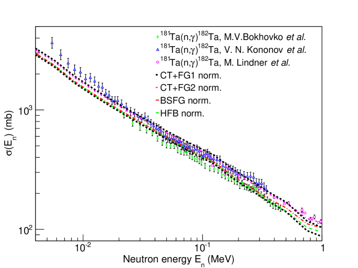
Figure 7: (Color online) The present ¹⁸¹Ta$(n,\gamma)$ cross section (bands) obtained from the ¹⁸¹Ta(d,p)¹⁸²Ta reaction, compared to previous measurements Bokhovko et al. (1991); Kononov et al. (1977); Lindner et al. (1976). The upper and lower band is indicated by the black-dotted line obtained using the CT+FG1 model.

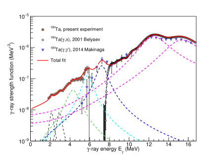
Figure 8: (Color online) ¹⁸¹Ta data from the 15 MeV ¹⁸¹Ta(d,d’)¹⁸¹Ta, ¹⁸¹Ta($\gamma$,$\gamma^{\prime}$) Makinaga et al. (2014), and ¹⁸¹Ta($\gamma,X$) Belyaev and Sinichkin (2001) reactions. Various resonances were identified (see text for details) and contribute to the total fit (red line) that best matches the experimental data.

The ¹⁸¹Ta(n,$\gamma$) cross sections have been extensively measured in time-of-flight Bokhovko et al. (1991); Kononov et al. (1977) and activation Lindner et al. (1976) measurements. It is interesting to compared these cross sections with those obtained from this work. The ¹⁸¹Ta(n,$\gamma$)¹⁸²Ta cross sections, $\sigma(E_{n})$, as a function of incident neutron energies for 0.004 keV to 1 MeV, taking into account the uncertainties affecting the $\gamma$SFs and the NLDs, have been calculated and are shown in Fig. 7. The cross sections obtained from the different normalizations yield very similar results. The ¹⁸¹Ta(n,$\gamma$)¹⁸²Ta cross sections exhibit a slight divergence below $10^{-2}$ MeV, but good agreement above $10^{-2}$ MeV with each other and with previous measurements. Similar results have been observed in Ref. Kheswa et al. (2017), where different normalisation models and spin distributions were explored in detail, yielding the same results. The agreement further validates that experimental NLDs and $\gamma$SFs can be used to obtain (n,$\gamma$) cross sections indirectly, and gives confidence in this technique to determine reliable (n,$\gamma$) cross sections for which direct measurement techniques are not currently viable e.g. Refs. Spyrou et al. (2014); Kheswa et al. (2015).

V Scissors resonance

The SR is a collective excitation mode dominated by single-particle events usually found at $E_{\gamma}=66\delta A^{-1/3}$, where $\delta$ is the quadrupole deformation parameter and $A$ is the nuclear mass Richter (1995). On a macroscopic level the SR may be described by the oscillation of the proton and neutron distributions against each other, similar to scissor blades. On a microscopic level the SR originates from transitions between Nilsson orbits of $\Delta\Omega=\pm 1$ with the same spherical $j$ component. The quantum number $\Omega$ is the projection of the total angular momentum onto the symmetry axis of the nucleus.

A splitting of the SR may be interpreted by means of $\gamma$ deformation along the three axes Iudice et al. (1985):

$$\begin{split}\omega_{1}=(\cos\gamma+\left(\frac{1}{\sqrt{3}}\right)\sin\gamma)\omega_{M1},\\ \omega_{2}=(\cos\gamma-\left(\frac{1}{\sqrt{3}}\right)\sin\gamma)\omega_{M1},\\ \omega_{3}=\omega_{M1}\frac{2}{\sqrt{3}}\sin\gamma,\end{split}$$ (10)

where $\omega_{1}$, $\omega_{2}$, and $\omega_{3}$ are the centroid energies of the individual SR components and $\omega_{M1}$ is the energy resonance centroid. Along the third axis, $\omega_{3}$ is located at low energies which is typically not within experimental reach of the Oslo Method. The splitting of the SR of the two higher-lying components can be calculated by Iudice et al. (1985):

$$\Delta\omega=\omega_{1}-\omega_{2}=\omega_{M1}\frac{2}{\sqrt{3}}\sin\gamma.$$ (11)

For axially symmetric nuclei ($\gamma$=0) the $\omega_{3}$ component is absent and the $\omega_{1}$ and $\omega_{2}$ components are degenerate.

Cross sections from ($\gamma$,$\gamma^{\prime}$) and ($\gamma,x$) reactions Makinaga et al. (2014); Belyaev and Sinichkin (2001) were converted to $\gamma$SF data with Eq. 9. The resonances of ¹⁸¹Ta for $E_{\gamma}<$ 9 MeV were fitted with standard Lorentzian functions, while for the components of the GEDR (purple dashed lines), the enhanced generalised Lorentzian functions were used, as shown in Fig. 8. The GEDR parameters were slightly modified from the average values of Refs. Capote et al. (2009); Mughabghab (2006) to better match the experimental data. From $(\gamma,\gamma^{\prime})$ data the enhanced $\gamma$SF, for 6 MeV $<E_{\gamma}<$ 8 MeV (dark-blue dashed line in Fig. 8) was suggested to be due to the E1 pygmy resonance Makinaga et al. (2014). A slight change in the gradient at around 4.5 MeV was noted for ¹⁸²Ta in Igashira et al. (1986), and this feature is also visible in our data and assumed to be a resonance at $\sim$ 4.3 MeV (green dashed line in Fig. 8). An additional unknown resonance at 5.8 MeV (light-blue dashed line in Fig. 8) was added so that the total fit matches the experimental data. The resonance parameters used for the fits in Fig. 8 are shown in table 3.

Table 3: The resonance centroid $\omega$, amplitude $\sigma$ and half width at half maximum $\Gamma$ used to fit the $\gamma$SF resonances. Enhanced generalised Lorentzian functions were used to fit the GEDR and standard Lorentzian functions were used for the other resonances.

$\omega$ (MeV)	$\sigma$ (mb)	$\Gamma$ (MeV)
2.2	0.2	0.4
2.9	0.3	0.5
4.4	2.3	1.3
5.8	8.5	1.0
7.3	21.8	1.1
12.7	340	2.8
15.6	320	3.6

The $\gamma$SF of ¹⁸¹Ta exhibits weak features at 2 MeV $<$ E_γ $<$ 3.5 MeV (black dashed lines in Fig. 8, which are found in the typical energy range for the SR Heyde et al. (2010). From this work the distinction between M1 and E1 is not possible but the assignment to the SR and its location in ¹⁸¹Ta is corroborated by previous measurements Wolpert et al. (1998); Angell et al. (2016).

The SR splits into two peaks, at $E_{\gamma}=$ 2.16 $\pm$ 0.04 MeV and $E_{\gamma}=$ 2.91 $\pm$ 0.05 MeV, which is consistent with the fragmentation observed in Ref. Wolpert et al. (1998). The average splitting of the SR peaks in ¹⁸¹Ta is $\Delta\omega=$ 0.75 $\pm$ 0.06 MeV. Using Eq. 11 a $\gamma$ deformation of 14.9^∘ $\pm$ 1.8^∘ is calculated. No additional strength is observed for ¹⁸⁰Ta or ¹⁸²Ta in the energy region of the SR.

Potential energy surface calculations for ^181,182Ta were performed with the Cranking Nilsson model plus Shell correction method Frauendorf (2000); Dimitrov et al. (2000); Xu et al. (2018) with pairing-gap values adopted from Ref. Möller et al. (1997) and are shown in Fig. 9. From these it is apparent that the ground-state configuration in ¹⁸¹Ta and ¹⁸²Ta exhibit a $\gamma$-axis minimum, between 0^∘-15^∘ and a deformation parameter of $\epsilon_{2}\approx$ 0.2. The deformation parameters $\delta$ and $\epsilon_{2}$ are the same to first order. From this, ^181,182Ta exhibit some softness towards $\gamma$ in the form of $\gamma$-vibrations and collectively prolate which is in agreement with $\gamma=14.9^{\circ}$ $\pm$ 1.8^∘ extracted from the splitting of the SR. This $\gamma$ deformation is also in agreement with those predicted in Refs. Hilaire and Girod (2007); Delaroche et al. (2003).

The neutron capture $\gamma$-ray spectra Igashira et al. (1986) of the odd-odd nuclei ¹⁴²Pr, ¹⁶⁰Tb, ¹⁶⁶Ho, ¹⁷⁶Lu, ¹⁸²Ta, and ¹⁹⁸Au are particularly interesting and can shed light on the above results. The large deformation of $\epsilon_{2}\sim$ 0.32 Hilaire and Girod (2007) in ¹⁶⁰Tb appears to produce a relatively localised strength at $E_{\gamma}$ = 2.5 MeV despite the two odd nucleons. Fragmentation increases for ¹⁶⁶Ho and ¹⁷⁶Lu as deformation is somewhat reduced to $\epsilon_{2}\sim$ 0.30 Hilaire and Girod (2007). For ¹⁴²Pr, ¹⁸²Ta, and ¹⁹⁸Au deformation is further reduced and may explain why the resonance is not identifiable. This is consistent with the proportionality of $B(M1)$ with the square of deformation Ziegler et al. (1990). While higher detection sensitivity Wolpert et al. (1998) reveals the presence, albeit fragmented, of the SR in ¹⁸¹Ta, the additional odd neutron and a slightly reduced deformation is sufficient to fragment the SR strength to a level that it is not observable in ¹⁸⁰Ta and ¹⁸²Ta.

Low-lying excitations of ¹⁸¹Ta were investigated using NRF experiments Angell et al. (2016); Wolpert et al. (1998). It was suggested that the SR was rather weak and splits into two parts. From our work, it can be concluded that a weak SR is observed with split centroids located at 2.16 MeV $\pm$ 0.04 MeV and 2.91 MeV $\pm$ 0.05 MeV, in agreement with NRF measurements Angell et al. (2016); Wolpert et al. (1998). The case of ¹⁸²Ta is similar to that of ^197,198Au Giacoppo et al. (2015) where no SR is observed.

The current results support nuclear triaxiality as the likely mechanism of SR splitting in ¹⁸¹Ta however there are alternative explanations. The SR splitting was proposed from microscopic calculations Balbutsev and Molodtsova (2013), which were able to explain the observed splitting in the actinide region Tornyi et al. (2014); Guttormsen et al. (2012, 2014); Laplace et al. (2016), where the triaxiality argument does not hold due to a mismatch of $B(M1)_{\omega 2}/B(M1)_{\omega 1}$, from the $B(M1)$ values of the individual SR components, and from the extracted $\gamma$ deformation Guttormsen et al. (2012). In these calculations the SR mode of protons oscillating against neutrons is accompanied by a lower-energy nuclear spin scissors mode where spin-up nucleons oscillate against spin-down nucleons.

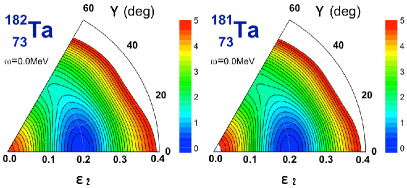
Figure 9: (Color online) Potential energy surface calculations with the Cranking Nilsson model plus Shell correction method for the ground states of ^181,182Ta, see text for details.

Despite systematic axially deformed QRPA calculations Goriely et al. (2016, 2018), the evolution of the SR across the nuclear chart is still not fully understood. For a complete understanding of the interplay of the SR with other nuclear structure properties, such as the coupling to unpaired nucleons and its dependence on nuclear shape, the persistence of the SR in transitional regions of the nuclear chart has to be investigated further.

VI Summary

The NLDs and $\gamma$SFs of ^180,181,182Ta were measured at the Oslo Cyclotron Laboratory. Six independent data sets from ¹⁸¹Ta(d,X) and ¹⁸¹Ta(³He,X) reactions were analysed with the Oslo Method. The total NLDs at the neutron separation energies and their uncertainties were calculated using three different models, the BSFG, CT+FG (1,2), and HFB plus Combinatorial models.

The comparison between the ¹⁸¹Ta(n,$\gamma$) cross-sections calculated with TALYS v1.9 using the measured NLD and $\gamma$SF and the results from direct measurements is satisfying and reinforces the appropriateness of using NLDs and $\gamma$SFs for the determination of neutron capture cross sections.

The $\gamma$ deformation of 14.9^∘ $\pm$ 1.8^∘ for ¹⁸¹Ta was calculated and this $\gamma$ softness, together with the unpaired nucleon, may be an explanation for a significant fragmentation of SR strength. Nuclear triaxiality may be considered as the likely mechanism of the observed SR splitting in ¹⁸¹Ta, but further experimental work and theoretical guidance on possible observables and specific experimental signatures for the spin-SR mode are desirable.

References

- Chadwick et al. (2011) M. B. Chadwick et al., Nucl. Data Sheets 112, 2887 (2011).
- (2) G. A. Bartholomew et al., Advances in Nuclear Physics Vol. 7 (edited by M. Baranger and E. Vogt (Plenum, New York, 1973)).
- Guttormsen et al. (2015) M. Guttormsen et al., Eur. Phys. J. A 51, 171 (2015).
- Moretto et al. (2015) L. Moretto et al., J. Phys.: Conf. Ser. 580, 012048 (2015).
- Hauser and Feshbach (1952) W. Hauser and H. Feshbach, Phys. Rev. 87, 366 (1952).
- Koning et al. (2008a) A. J. Koning et al., EDP sciences; eds O. Bersillon et. al., 211 (2008a), see also www.talys.eu.
- Arnould et al. (2007) M. Arnould, S. Goriely, and K. Takahashi, Phys. Rep. 97, 450 (2007).
- Goriely (1998) S. Goriely, Phys. Lett. B 436, 10 (1998).
- Guttormsen et al. (2017) M. Guttormsen et al., Phys. Rev. C 96, 024313 (2017).
- Kheswa et al. (2017) B. V. Kheswa et al., Phys. Rev. C 95, 045805 (2017).
- Larsen et al. (2016) A. C. Larsen et al., Phys. Rev. C 93, 045810 (2016).
- Dimitriou et al. (2018) P. Dimitriou et al., EPJ Web Conf. 178, 06005 (2018).
- Suzuki and Rowe (1977) T. Suzuki and D. Rowe, Nucl. Phys. A289, 461 (1977).
- Iudice and Palumbo (1978) N. L. Iudice and F. Palumbo, Phys. Rev. Lett. 41, 1532 (1978).
- Iudice and Palumbo (1979) N. L. Iudice and F. Palumbo, Nucl. Phys. A326, 461 (1979).
- Iachello (1981) F. Iachello, Nucl. Phys. A358, 89c (1981).
- Bohle et al. (1984a) D. Bohle et al., Phys. Lett. B 137, 27 (1984a).
- Bohle et al. (1984b) D. Bohle et al., Phys. Lett. B 148, 260 (1984b).
- Iudice et al. (1985) N. L. Iudice et al., Phys. Lett. B 161, 18 (1985).
- Heyde et al. (2010) K. Heyde, P. von Neumann-Cosel, and A. Richter, Rev. Mod. Phys. 82, 2365 (2010).
- Schwengner et al. (1997) R. Schwengner et al., Nucl. Phys. A620, 277 (1997).
- Fransen et al. (1999) C. Fransen et al., Phys. Rev. C 59, 2264 (1999).
- Maser et al. (1996) H. Maser et al., Phys. Rev. C 54, R2129 (1996).
- von Brentano et al. (1996) P. von Brentano et al., Phys. Rev. Lett. 76, 2029 (1996).
- Kneissl et al. (1996) U. Kneissl, H. H. Pitz, and A. Zilges, Prog. Part. Nucl. Phys. 37, 349 (1996).
- Baramsai (2015) B. Baramsai, EPJ Web of Conferences 93, 01037 (2015).
- Schiller et al. (2000) A. Schiller et al., Nucl. Instrum. Methods Phys. Res. A 447, 498 (2000).
- Guttormsen et al. (2012) M. Guttormsen et al., Phys. Rev. Lett. 109, 162503 (2012).
- Guttormsen et al. (2014) M. Guttormsen et al., Phys. Rev. C 89, 014302 (2014).
- Tornyi et al. (2014) T. G. Tornyi et al., Phys. Rev. C 89, 044323 (2014).
- Laplace et al. (2016) T. Laplace et al., Phys. Rev. C 93, 014323 (2016).
- Guttormsen et al. (2011) M. Guttormsen et al., Nucl. Instrum. Methods Phys. Res. A 648, 168 (2011).
- Guttormsen et al. (1990) M. Guttormsen et al., Phys. Scr. T32, 54 (1990).
- Larsen et al. (2011) A. C. Larsen et al., Phys. Rev. C 83, 034315 (2011).
- Guttormsen et al. (1996) M. Guttormsen et al., Nucl. Instrum. Methods Phys. Res. A 374, 371 (1996).
- Guttormsen et al. (1987) M. Guttormsen, T. Ramsy, and J. Rekstad, Nucl. Instrum. Methods Phys. Res. A 255, 518 (1987).
- Brink (1955) D. Brink, Ph.D. thesis (Oxford University unpublished, 1955).
- (38) Brookhaven National Laboratory, “National nuclear data center on-line data service,” http://www.nndc.bnl.gov, retrieved 2015.
- Gilbert and Cameron (1965) A. Gilbert and A. G. W. Cameron, Can. J. of Phys. 43, 1446 (1965).
- Koning and Rochman (2012) A. J. Koning and D. Rochman, Nucl. Data Sheets 113, 2841 (2012).
- Goriely et al. (2008) S. Goriely, S. Hilaire, and A. Koning, Phys. Rev. C 78, 064307 (2008).
- Bohr and Mottelson (1969) A. Bohr and B. Mottelson, Nuclear structure, 1st ed. (Benjamin, New York, 1969).
- Capote et al. (2009) R. Capote et al., Nucl. Data Sheets. 110, 3107 (2009). Available online at http://www-nds.iaea.org/RIPL-3/ (2009).
- Mughabghab (2006) S. F. Mughabghab, Atlas of Neutron Resonance, 5th ed. (Elsevier Science, Amsterdam, 2006).
- von Egidy and Bucurescu (2009) T. von Egidy and D. Bucurescu, Phys. Rev. C 80 (2009).
- Koning et al. (2008b) A. J. Koning, S. Hilaire, and S. Goriely, Nucl. Phys. A810, 13 (2008b).
- Ericson (1959) T. Ericson, Nucl. Phys. A11, 481 (1959).
- Dilg et al. (1973) W. Dilg et al., Nucl. Phys. A217, 269 (1973).
- Kopecky and Uhl (1990) J. Kopecky and M. Uhl, Phys. Rev. C 41, 1941 (1990).
- Igashira et al. (1986) M. Igashira et al., Nucl. Phys. A457, 301 (1986).
- Utsunomiya et al. (2003) H. Utsunomiya et al., Phys. Rev. C 67, 015807 (2003).
- Bergère et al. (1968) R. Bergère, H. Beil, and A. Veyssière, Nucl. Phys. A121, 463 (1968).
- Makinaga et al. (2014) A. Makinaga et al., Phys. Rev. C 90, 044301 (2014).
- Goriely et al. (2016) S. Goriely et al., Phys. Rev. C 94, 044306 (2016).
- Goriely et al. (2018) S. Goriely et al., Phys. Rev. C 98, 014237 (2018).
- Kopecky et al. (2017) J. Kopecky et al., Phys. Rev. C 95, 054317 (2017).
- Koning and Delaroche (2003) A. Koning and J. Delaroche, Nucl. Phys. A703, 231 (2003).
- Hofmann et al. (1975) H. Hofmann et al., Ann. Phys. (N.Y.) 90, 403 (1975).
- Bokhovko et al. (1991) M. V. Bokhovko et al., Conf. on Nucl. Data for Sci. and Technol. Jeulich , 62 (1991).
- Kononov et al. (1977) V. N. Kononov et al., Sov. J. Nucl. Phys. 26, 500 (1977).
- Lindner et al. (1976) M. Lindner et al., Nucl. Sci. Eng. 59, 381 (1976).
- Belyaev and Sinichkin (2001) S. N. Belyaev and V. P. Sinichkin, Workshop on beam dynamics and optimization, Saratov , 81 (2001).
- Spyrou et al. (2014) A. Spyrou et al., Phys. Rev. Lett. 113, 232502 (2014).
- Kheswa et al. (2015) B. V. Kheswa et al., Phys. Lett. B 744, 268 (2015).
- Richter (1995) A. Richter, Prog. Part. Nucl. Phys. 34, 261 (1995).
- Wolpert et al. (1998) A. Wolpert et al., Phys. Rev. C 58, 765 (1998).
- Angell et al. (2016) C. T. Angell et al., Phys. Rev. Lett. 117, 142501 (2016).
- Frauendorf (2000) S. Frauendorf, Nucl. Phys. A667, 115 (2000).
- Dimitrov et al. (2000) V. Dimitrov, S. Frauendorf, and F. Dönau, Phys. Rev. Lett. 84, 5732 (2000).
- Xu et al. (2018) Q. Xu et al., Eur. Phys. J. A 54, 83 (2018).
- Möller et al. (1997) P. Möller, J. R. Nix, and K. L. Kratz, At. Data Nucl. Data Tables 66, 131 (1997).
- Hilaire and Girod (2007) S. Hilaire and M. Girod, Eur. Phys. J A 33, 237 (2007).
- Delaroche et al. (2003) J. Delaroche et al., Phys. Rev. C 81, 014303 (2003).
- Ziegler et al. (1990) W. Ziegler et al., Phys. Rev. Lett. 65, 2515 (1990).
- Giacoppo et al. (2015) F. Giacoppo et al., Phys. Rev. C 91, 054327 (2015).
- Balbutsev and Molodtsova (2013) E. Balbutsev and I. Molodtsova, Phys. Rev. C 88, 014306 (2013).