A Deterministic Algorithm for the Capacity of Finite-State Channels  

Abstract

We propose two modified versions of the classical gradient ascent method to compute the capacity of finite-state channels with Markovian inputs. For the case that the channel mutual information is strongly concave in a parameter taking values in a compact convex subset of some Euclidean space, our first algorithm proves to achieve polynomial accuracy in polynomial time and, moreover, for some special families of finite-state channels our algorithm can achieve exponential accuracy in polynomial time under some technical conditions. For the case that the channel mutual information may not be strongly concave, our second algorithm proves to be at least locally convergent.

1 Introduction

As opposed to a discrete memoryless channel, which features a single state and thereby can be characterized by input and output random variables only, the characterization of a finite-state channel has to resort to additional state random variables. Encompassing discrete memoryless channels as special cases, finite-state channels have long been used in a wide range of communication scenarios where the current behavior of the channel may be affected by its past. Among many others, conventional examples of such channels include inter-symbol interference channels [8], partial response channels [22, 23] and Gilbert-Elliott channels [21].

While it is well-known that the Blahut-Arimoto algorithm [2, 4] can be used to efficiently compute the capacity of a discrete memoryless channel, the computation of the capacity of a general finite-state channel has long been a notoriously difficult problem, which has been open for decades. The difficulty of this problem may be justified by the widely held (yet not proven) belief that the capacity of a finite-state channel may not be achieved by any finite-order Markovian input, and an increase of the memory of the input may lead to an increase of the channel capacity.

We are mainly concerned with finite-state channels with Markov processes of a fixed order as their inputs. Possibly an unavoidable compromise we have to make in exchange for progress in computing the capacity, the extra fixed-order assumption imposed on the input processes is also necessary for the situation where the channel input has to satisfy certain constraints, notably finite-type constraints [19] that are commonly used in magnetic and optical recording. On the other hand, the focus on Markovian inputs can also be justified by the known fact that the Shannon capacity of an indecomposable finite-state channel [9] can be approximated by the Markov capacity with increasing orders (see Theorem $2.1$ of [18]). Recently, there has been some progress in computing the capacity of finite-state channels with such input constraints. Below we only list the most relevant work in the literature, and we refer the reader to [12] for a comprehensive list of references. In [15], the Blahut-Arimoto algorithm was reformulated into a stochastic expectation-maximization procedure and a similar algorithm for computing the lower bound of the capacity of finite-state channels was proposed, which led to a generalized Blahut-Arimoto algorithm [24] that proves to compute the capacity under some concavity assumptions. More recently, inspired by ideas in stochastic approximation, a randomized algorithm was proposed [12] to compute the capacity under weaker concavity assumptions, which can be verified to hold true for families of practical channels [14, 16]. Both of the above-mentioned algorithms, however, are of a randomized nature (a feasible implementation of the generalized Blahut-Arimoto algorithm will necessitate a randomization procedure). By comparison, among many other advantages, our algorithms, which are deterministic in nature, can be used to derive accurate estimates on the channel capacity, as evidenced by the tight bounds in Section 3.2.

In this paper, we first deal with the case that the mutual information of the finite-state channel is strongly concave in a parameter taking values in a compact convex subset of some Euclidean space, for which we propose our first algorithm that proves to converge to the channel capacity exponentially fast. This algorithm largely follows the spirit of the classical gradient ascent method. However, unlike the classical case, the lack of an explicit expression for our target function and the boundedness of the variable domain (without an explicit description of the boundary) pose additional challenges. To overcome the first issue, a convergent sequence of approximating functions (to the original target function) is used instead in our treatment; meanwhile, an additional check condition is also added to ensure that the iterates stay inside the given variable domain. A careful convergence analysis has been carried out to deal with the difficulties caused by such modifications. This algorithm is efficient in the sense that, for a general finite-state channel (satisfying the above-mentioned concavity condition and some additional technical conditions), it achieves polynomial accuracy in polynomial time (see Theorem 3.12), and for some special families of finite-state channels it achieves exponential accuracy in polynomial time (see Section 3.2).

It is well known that the mutual information of a finite-state channel may not be concave under the natural parametrization in several examples; see, e.g., [14, 16]. Another modification of the classical gradient ascent method is proposed to handle this challenging scenario. Similar to our first algorithm, our second one replaces the original target function with a sequence of approximating functions, which unfortunately renders conventional methods such as the Frank-Wolfe method (see, e.g., [3]) or methods using the Łojasiewicz inequality (see, e.g., [1]) inapplicable. To address this issue, among other subtle modifications, we impose an extra check in the algorithm to slow down the pace “a bit” to avoid an immature convergence to a non-stationary point but “not too much” to ensure the local convergence.

As variants of the classical gradient ascent method, our algorithms can be applied to any sequence of convergent functions, so they can be of particular interest in information theory since many information-theoretic quantities are defined as the limit of their finite-block versions. On the other hand though, we would like to add that our algorithms are actually stated in much more general settings and may have potential applications in optimization scenarios where the target functions are difficult to compute but amenable to approximations.

The remainder of this paper is organized as follows. In Section 2, we describe our channel model in great detail. Then, we present our first algorithm (Algorithm 3.3) in Section 3 and analyze its convergence behavior in Section 3.1 under some strong concavity assumptions. Applications of this algorithm for computing the capacity of finite-state channels under concavity assumptions will be discussed in Section 3.2. In particular, in this section, we show that the estimation of the channel capacity can be improved by increasing the Markov order of the input process in some examples. In Section 4, our second algorithm (Algorithm 4.2) is presented, which proves to be at least locally convergent. Finally, in Section 4.2, our second algorithm is applied to a Gilbert-Elliott channel where the concavity of the channel mutual information rate in the natural parametrization is not known, and yet fast convergence behavior is observed.

In the remainder of this paper, the base of the logarithm is assumed to be $e$.

2 Channel Model and Problem Formulation

In this section, we introduce the channel model considered in this paper, which is essentially the same as that in [12, 24].

As mentioned before, we are concerned with a discrete-time finite-state channel with a Markovian channel input. Let $X=\{X_{n}:n=1,2,\dots\}$ denote the channel input process, which is often assumed to be a first-order stationary Markov chain  over a finite alphabet $\mathcal{X}$, and let $Y=\{Y_{n}:n=1,2,\dots\}$ and $S=\{S_{n}:n=0,1,\dots\}$ denote the channel output and state processes over finite alphabets $\mathcal{Y}$ and $\mathcal{S}$, respectively.

Let $\Pi$ be the set of all the stochastic matrices of dimension $|\mathcal{X}|\times|\mathcal{X}|$. For any finite set $F\subseteq\mathcal{X}^{2}$ and any $\delta>0$, define

$$\Pi_{F,\delta}\triangleq\{A\in\Pi:A_{ij}=0,~{}~{}\mbox{for}~{}(i,j)\in F~{}~{}\mbox{and}~{}A_{ij}\geq\delta~{}~{}\mbox{otherwise}\}.$$

It can be easily verified that if one of the matrices from $\Pi_{F,\delta}$ is primitive, then all matrices from $\Pi_{F,\delta}$ will be primitive, in which case, as elaborated on in [12], $F$ gives rise to a so-called mixing finite-type constraint. Such a constraint has been widely used in data storage and magnetic recoding [20], the best known example being the so-called $(d,k)$-run length limited (RLL) constraint over the alphabet $\{0,1\}$, which forbids any sequence with fewer than $d$ or more than $k$ consecutive zeros in between two successive $1$’s.

The following conditions will be imposed on the finite-state channel described above:

1. There exist $F\subseteq\mathcal{X}^{2}$ and $\delta>0$ such that the transition probability matrix of $X$ belongs to $\Pi_{F,\delta}$, each element of which is a primitive matrix.

2. $(X,S)$ is a first-order stationary Markov chain whose transition probabilities satisfy

   $$p(x_{n},s_{n}|x_{n-1},s_{n-1})=p(x_{n}|x_{n-1})p(s_{n}|x_{n},s_{n-1}),\quad n=1,2,\dots,$$

   where $p(s_{n}|x_{n},s_{n-1})>0$ for any $s_{n-1},s_{n},x_{n}$.

3. The channel is stationary and characterized by

   $$p(y_{n}|y_{1}^{n-1},x_{1}^{n},s_{1}^{n-1})=p(y_{n}|x_{n},s_{n-1})>0,\quad n=1,2,\dots,$$

   that is, conditioned on the pair $(x_{n},s_{n-1})$, the output $Y_{n}$ is statistically independent of all inputs, outputs and states prior to $X_{n},Y_{n}$ and $S_{n-1}$, respectively.

As elaborated on in Remark 4.1 of [12], a finite-state channel specified as above is indecomposable. Therefore, assuming that the input $X$ (or, more precisely, the transition probability matrix of $X$) is analytically parameterized by a finite-dimensional parameter $\theta$ in a compact convex subset $\Theta$ of some Euclidean space (such a parameterization exists thanks to the stationarity of $X$), we can express the capacity of the above channel as

$$C=\max_{\theta\in\Theta}I(X(\theta);Y(\theta))=\max_{\theta\in\Theta}\lim_{k\to\infty}I_{k}(X(\theta);Y(\theta)),$$ (1)

where

$$I_{k}(X(\theta);Y(\theta))\triangleq\frac{H(X_{1}^{k}(\theta))+H(Y_{1}^{k}(\theta))-H(X_{1}^{k}(\theta),Y_{1}^{k}(\theta))}{k}.$$ (2)

Moreover, it has also been shown in [12] that $I_{k}(X(\theta);Y(\theta))$ (resp., its derivatives) converges to $I(X(\theta);Y(\theta))$ (resp., the corresponding derivatives) exponentially fast in $k$ under Assumptions (2.$a$), (2.$b$) and (2.$c$). Hence, although the value of the target function $I(X(\theta);Y(\theta))$ cannot be exactly computed, it can be approximated by the function $I_{k}(X(\theta);Y(\theta))$, which has an explicit expression, within an error exponentially decreasing in $k$.

Instead of merely solving (1), we will deal with the following slightly more general problem

$$\max f(\theta)=\lim_{k\rightarrow\infty}f_{k}(\theta)$$

$$\mbox{subject to}\quad\theta\in\Theta,$$ (3)

under the following assumptions:

1. $\Theta$ is a compact convex subset of $\mathbb{R}^{d}$ for some $d\in\mathbb{N}$ with nonempty interior $\Theta^{\circ}$ and boundary $\partial\Theta$;

2. $f(\theta)$ and all $f_{k}(\theta)$, $k\geq 0$, are continuous on $\Theta$ and twice continuously differentiable in $\Theta^{\circ}$;

3. there exist $M_{0}>0$, $N>0$ and $0<\rho<1$ such that for all $k\geq 1$, $\theta\in\Theta^{\circ}$ and $\ell=0,1,2$, it holds true that $||f_{0}^{(\ell)}(\theta)||_{2}\leq M_{0}$ and

   $$||f_{k}^{(\ell)}(\theta)-f_{k-1}^{(\ell)}(\theta)||_{2}\leq N\rho^{k},\quad\quad||f_{k}^{(\ell)}(\theta)-f^{(\ell)}(\theta)||_{2}\leq N\rho^{k},$$ (4)

   where the superscript ^(ℓ) denotes the $\ell$-th order derivative and $||\cdot||_{2}$ denotes the Frobenius norm of a vector/matrix.

Obviously, if we set $f_{k}(\theta)=I_{k}(X(\theta);Y(\theta))$ and assume that $X(\theta)$ analytically parameterized by some $\theta\in\Theta$, then (2) boils down to (1).

When the target function $f(\theta)$ has an explicit expression and $\Theta$ is characterized by finitely many twice continuously differentiable constraints, the optimization problem (3) can be effectively dealt with via, for example, the classical gradient ascent method [5] or the Frank-Wolfe method [3] or their numerous variants. However, feasible implementations and executions of these algorithms usually hinge on explicit descriptions of $\Theta$ and $\nabla f$, both of which can be rather intricate in our setting.

Before moving to the next two sections to present our algorithms, we make some observations about the sequence $\{f_{k}(\theta)\}_{k=0}^{\infty}$. It immediately follows from the uniform boundedness of $||f_{0}^{(\ell)}(\theta)||_{2}$ and the inequality (4) that there exists $M>0$ such that for all $k\geq 0$, $\ell=0,1,2$ and $\theta\in\Theta^{\circ}$,

$$||f_{k}^{(\ell)}(\theta)||_{2}\leq M.$$ (5)

In particular, for any $\theta\in\Theta^{\circ}$, when $\ell=2$, $f_{k}^{(\ell)}(\theta)=\nabla^{2}f_{k}(\theta)$ is a symmetric matrix whose spectral norm is given by

$$|||\nabla^{2}f_{k}(\theta)|||_{2}\triangleq\sup_{\mathbf{x}\neq 0}\frac{||\nabla^{2}f_{k}(\theta)\cdot\mathbf{x}||_{2}}{||\mathbf{x}||_{2}}=|\lambda_{1}(\theta)|,$$

where $\lambda_{1}$ denotes the largest (in modulus) eigenvalue of $\nabla^{2}f_{k}(\theta)$. Hence, the inequality (5) and the easily verifiable fact that $|||\nabla^{2}f_{k}(\theta)|||_{2}\leq||\nabla^{2}f_{k}(\theta)||_{2}$ imply

$$-M\mathbb{I}_{d}\preceq\nabla^{2}f_{k}(\theta)\preceq M\mathbb{I}_{d}$$ (6)

for any $k$ and any $\theta\in\Theta^{\circ}$, where $\mathbb{I}_{d}$ denotes the $d\times d$ identity matrix, and for two matrices $A,B$ of the same dimension, by $A\preceq B$, we mean that $B-A$ is a positive semidefinite matrix. The existence of the constant $M$ in (6) will be crucial for implementing our algorithms.

3 The First Algorithm: with Concavity

Throughout this section, we assume that $f(\theta)$ is strongly concave, i.e., there exists $m>0$ such that for all $\theta\in\Theta^{\circ},$

$$\nabla^{2}f(\theta)\preceq-m\mathbb{I}_{d},$$ (7)

and moreover

$$f\mbox{ achieves its unique maximum in }\Theta^{\circ}.$$ (8)

We will present our first algorithm to solve the optimization problem (2). As mentioned before, the algorithm is in fact a modified version of the classical gradient ascent algorithm, whereas its convergence analysis is more intricate than the classical one. To overcome the issue that the target function $f(\theta)$ may not have an explicit expression we capitalize on the fact that it can be well approximated by $\{f_{k}(\theta)\}_{k=0}^{\infty}$, which will be used instead to compute the estimates in each iteration.

Before presenting our algorithm, we need the following lemma, which, as evidenced later, is important in initializing and analyzing our first algorithm.

Lemma 3.1.

There exists a non-negative integer $k_{0}$ such that

1. $\displaystyle\frac{(N+M)M\rho^{k_{0}+1}+2N\rho^{k_{0}+1}}{1-\rho}\leq\frac{\delta}{8}$ and $N\rho^{k_{0}}\leq\displaystyle\frac{\delta}{8}$, where $\delta\triangleq\max\limits_{\theta\in\Theta}f(\theta)-\max\limits_{\theta\in\partial\Theta}f(\theta)>0$.

2. For any $k\geq k_{0}$, $f_{k}(\theta)$ is strongly concave and has a unique maximum in $\Theta^{\circ}$; and moreover, we have

   $$\sup_{k\geq k_{0}}||\theta_{k}^{*}-\theta^{*}||_{2}+\frac{d^{1/2}\rho^{k_{0}}}{1-\rho}<dist(\theta^{*},\partial\Theta),$$ (9)

   where $\theta^{*}$ denotes the unique maximum point of $f$ and $\theta^{*}_{k}$ denotes the unique maximum point of $f_{k}$.

3. There exists $y_{0}\in\mathbb{R}$ such that for all $k\geq k_{0}$,

   $$\emptyset\subsetneq B_{k}\subseteq C_{k}\subseteq\Theta^{\circ}\quad\mbox{and}\quad dist(C_{k},\partial\Theta)>0,$$

   where

   $$B_{k}\triangleq\{x\in\Theta:f_{k}(x)\geq y_{0}\}\quad\mbox{and}\quad C_{k}\triangleq\left\{x\in\Theta:f_{k}(x)\geq y_{0}-\frac{\delta}{8}\right\}.$$

Proof.

Since $(a)$ trivially holds for sufficiently large $k_{0}$, we will omit its proof and proceed to prove $(b)$. Towards this end, note that according to (4) and (7), it holds true that for sufficiently large $k$, each $f_{k}$ is strongly concave. Noting that $f(\theta^{*})-\max_{\theta\in\partial\Theta}f(\theta)=\delta$, we deduce from $(a)$ and (4) that for $k$ large enough,

$$\max_{\theta\in\Theta}f_{k}(\theta)-\max_{\theta\in\partial\Theta}f_{k}(\theta)\geq f_{k}(\theta^{*})-\max_{\theta\in\partial\Theta}f(\theta)-\frac{\delta}{8}\geq f(\theta^{*})-\max_{\theta\in\partial\Theta}f(\theta)-\frac{\delta}{4}=\frac{3\delta}{4}>0.$$ (10)

Hence, for $k$ sufficiently large, $f_{k}$ achieves its unique maximum at $\theta_{k}^{*}\in\Theta^{\circ}$.

We now prove that $\theta_{k}^{*}\rightarrow\theta^{*}$ as $k\rightarrow\infty$. To see this, observe that (4) implies the uniform convergence of $f_{k}$ to $f$, i.e., for any $\varepsilon>0$, there exists $K>0$ such that for any $k>K$ and any $\theta\in\Theta$, $f(\theta)-\varepsilon\leq f_{k}(\theta)\leq f(\theta)+\varepsilon.$ In particular, for $k>K$, we have

$$f(\theta^{*})-\varepsilon\leq f_{k}(\theta^{*})\leq f_{k}(\theta_{k}^{*})\leq f(\theta_{k}^{*})+\varepsilon\leq f(\theta^{*})+\varepsilon,$$

which further implies that $f_{k}(\theta_{k}^{*})\rightarrow f(\theta^{*})$ as $k\to\infty$. It then follows from the triangle inequality that

$$f(\theta_{k}^{*})\rightarrow f(\theta^{*}),~{}~{}\mbox{ as $k\to\infty$.}$$ (11)

Now, by the Taylor series expansion, there exists some $\tilde{\theta}\in\Theta^{\circ}$ such that

$$f(\theta_{k}^{*})-f(\theta^{*})=\nabla f(\theta^{*})^{T}(\theta_{k}^{*}-\theta^{*})+(\theta_{k}^{*}-\theta^{*})^{T}\nabla^{2}f(\tilde{\theta})(\theta_{k}^{*}-\theta^{*}).$$ (12)

Since $\nabla f(\theta^{*})=0$ and $\nabla^{2}f(\tilde{\theta})\preceq-m\mathbb{I}_{d}$ according to (7), it follows from (11) and (12) that $\theta_{k}^{*}\rightarrow\theta^{*}$ as $k\rightarrow\infty$, as desired.

It then immediately follows that $||\theta_{k}^{*}-\theta^{*}||_{2}+d^{1/2}\rho^{k}/(1-\rho)\rightarrow 0$ as $k\rightarrow\infty$. Observing that $dist(\theta^{*},\partial\Theta)>0$ (since $\theta^{*}\in\Theta^{\circ}$), we infer that (9) holds for sufficiently large $k$. Hence, $(b)$ will be satisfied as long as $k_{0}$ is sufficiently large.

We now show that $(c)$ also holds for sufficiently large $k_{0}$. From the definition of $\delta$, there exists $y_{0}$ such that $\max_{\theta\in\partial\Theta}f(\theta)+\frac{\delta}{4}<y_{0}<\max_{\theta\in\Theta}f(\theta)-\frac{\delta}{4}$. From (4), using the same logic as that used to derive (10), we infer that for sufficiently large $k$,

$$\max_{\theta\in\partial\Theta}f_{k}(\theta)<y_{0}-\frac{\delta}{8}<y_{0}<\max_{\theta\in\Theta}f_{k}(\theta).$$ (13)

According to $(b)$ and the fact that $\theta_{k}^{*}\in\Theta^{\circ}$, which follows from (13), we deduce that $\emptyset\subsetneq B_{k}\subseteq C_{k}\subseteq\Theta^{o}$ and $dist(C_{k},\partial\Theta)>0$ with

$$C_{k}\triangleq\left\{x:f_{k}(x)\geq y_{0}-\frac{\delta}{8}\right\}\quad\mbox{and}\quad B_{k}\triangleq\{x:f_{k}(x)\geq y_{0}\}.$$

Therefore, $(c)$ is valid as long as $k_{0}$ is sufficiently large. Finally, choosing a larger $k_{0}$ if necessary, we conclude that there exists $k_{0}$ such that $(a)$, $(b)$ and $(c)$ are all satisfied. ∎

Remark 3.2.

We remark that, for any $k\geq k_{0}$, each $B_{k}$ specified as above has a non-empty interior, which is due to the strict inequality (13) and the continuity of $f_{k}$.

We are now ready to present our first algorithm, which modifies the classical gradient ascent method in the following manner: Instead of using $\nabla f$ to find a feasible direction, we use $\nabla f_{k}$ as the ascending direction in the $k$-th iteration and then pose additional check conditions for a careful choice of the step size. Note that such modifications make the convergence analysis more difficult compared to the classical case, as elaborated on in the next subsection.

Algorithm 3.3.

(The first modified gradient ascent algorithm)

Step $0$. Choose $k_{0}$ such that Lemma 3.1 $(a)$-$(c)$ hold. Set $k=0$, $g_{0}=f_{k_{0}}$ and choose $\alpha\in(0,0.5)$, $\beta\in(0,1)$ and $\theta_{0}\in\Theta^{\circ}$ such that $\theta_{0}\in B_{k_{0}}$ and $\nabla g_{0}(\theta_{0})\neq 0$.

Step $1$. Increase $k$ by $1$, and set $t=1$, $g_{k}=f_{k_{0}+k}$.

Step $2$. If $\nabla g_{k-1}(\theta_{k-1})=0$, set

$$\tau=\theta_{k-1}+t\nabla g_{k-1}(\theta_{k-1}+\rho^{k+k_{0}}\mathbf{1}),$$

where $\mathbf{1}$ denotes the all-one vector in $\mathbb{R}^{d}$; otherwise, set

$$\tau=\theta_{k-1}+t\nabla g_{k-1}(\theta_{k-1}).$$

If $\tau\not\in\Theta$ or

$$g_{k}(\tau)<g_{k}(\theta_{k-1})+\alpha t||\nabla g_{k-1}(\theta_{k-1})||_{2}^{2}-(N+M)Mt\rho^{k+k_{0}},$$

set $t=\beta t$ and go to Step $2$, otherwise set $\theta_{k}=\tau$ and go to Step $1$.

Remark 3.4.

It is obvious from the definition of $g_{k}$ that as $k$ tends to infinity, $g_{k}$ (resp., its first and second order derivatives) converges to $f$ (resp., its first and second order derivatives) exponentially with the same constant as in (4).

Remark 3.5.

The existence of $\theta_{0}$ in Step $0$ can be justified by Lemma 3.1 $(c)$.

Remark 3.6.

We point out that in Step 2 of Algorithm 3.3, for any $k\geq 1$, the point $\theta_{k-1}+\rho^{k+k_{0}}\mathbf{1}$ will always lie in $\Theta^{\circ}$. To see this, note that, according to Algorithm 3.3, $\tau=\theta_{k-1}+t\nabla g_{k-1}(\theta_{k-1}+\rho^{k+k_{0}}\mathbf{1})$ only if $\theta_{k-1}$ is the maximum point of $g_{k-1}=f_{k+k_{0}-1}$, i.e., $\theta_{k-1}=\theta_{k+k_{0}-1}^{*}$. However, by Lemma 3.1 $(b)$, these points always satisfy (9), which immediately implies that $\theta_{k-1}+\rho^{k+k_{0}}\mathbf{1}\in\Theta^{\circ}$ for all $k\geq 1$.

Remark 3.7.

For technical reasons that will be made clear in the next section, $\alpha$ is chosen within $(0,0.5)$ to ensure the convergence of the algorithm. In Step $2$ of algorithm 3.3, the case that $\nabla g_{k-1}(\theta_{k-1})=0$ is singled out for special treatment to prevent the algorithm from getting trapped at the maximum point of $f_{k-1}$ for a fixed $k$, which may be still far away from the maximum point of $f$.

3.1 Convergence Analysis

As mentioned earlier, compared to the classical gradient ascent method, Algorithm 3.3 poses additional challenges for convergence analysis. The main difficulties come from the two check conditions in Step 2: the “perturbed” Armijo condition (see, e.g., Chapter 2 of [3] for more details)

$$g_{k}(\tau)\geq g_{k}(\theta_{k-1})+\alpha t||\nabla g_{k-1}(\theta_{k-1})||_{2}^{2}-(N+M)Mt\rho^{k+k_{0}}$$

may break the monotonicity of the sequence $\{g(\theta_{k})\}_{k=0}^{\infty}$ which would have been used to simplify the convergence analysis in the classical case; and the extra check condition $\tau\in\Theta$ ($\tau$ depends on $k$) forces us to seek uniform control (over all $k$) of the time used to ensure the validity of this condition in each iteration. In the remainder of this section, we deal with these problems and examine the convergence behavior of Algorithm 3.3. In a nutshell, we will prove that our algorithm converges exponentially in time under some strong concavity assumptions.

Note that the variable $k$ as in Algorithm 3.3 actually records the number of times that Step $1$ has been executed at the present moment. To facilitate the analysis of our algorithm, we will put it into an equivalent form, where an additional variable $n$ is used to record the number of times that Step $2$ has been executed.

Below is Algorithm 3.3 rewritten with the additional variable $n$.

Algorithm 3.8.

(An equivalent form of Algorithm 3.3)

Step $0$. Choose $k_{0}$ such that Lemma 3.1 $(a)$-$(c)$ hold. Set $n=0,k=0,\hat{g}_{0}=g_{0}=f_{k_{0}}$, and choose $\alpha\in(0,0.5),\beta\in(0,1)$ and $\hat{\theta}_{0}\in\Theta^{\circ}$ such that $\hat{\theta}_{0}\in B_{k_{0}}$ and $\nabla\hat{g}_{0}(\hat{\theta}_{0})\neq 0$.

Step $1$. Increase $k$ by $1$, and set $t=1$, $g_{k}=f_{k_{0}+k}$.

Step $2$. Increase $n$ by $1$. If $\nabla\hat{g}_{n-1}(\hat{\theta}_{n-1})=0$, set

$$\tau=\hat{\theta}_{n-1}+t\nabla\hat{g}_{n-1}(\hat{\theta}_{n-1}+\rho^{k+k_{0}}\mathbf{1});$$ (14)

otherwise, set

$$\tau=\hat{\theta}_{n-1}+t\nabla\hat{g}_{n-1}(\hat{\theta}_{n-1}).$$ (15)

If $\tau\not\in\Theta^{\circ}$ or

$$g_{k}(\tau)<g_{k}(\hat{\theta}_{n-1})+\alpha t||\nabla\hat{g}_{n-1}(\hat{\theta}_{n-1})||_{2}^{2}-(N+M)Mt\rho^{k+k_{0}},$$ (16)

then set $\hat{\theta}_{n}=\hat{\theta}_{n-1},\hat{g}_{n}=\hat{g}_{n-1},t=\beta t$ and go to Step $2$; otherwise, set $\hat{\theta}_{n}=\tau,\hat{g}_{n}=g_{k}$ and go to Step $1$.

Remark 3.9.

Let $n_{0}=0$, and for any $k\geq 1$, recursively define

$$n_{k}=\inf\{n>n_{k-1}:\hat{\theta}_{n}\neq\hat{\theta}_{n-1}\}.$$

Then, one verifies that for any $k\geq 0$, it holds true that $\hat{\theta}_{n_{k}}=\theta_{k}$, $\hat{g}_{n_{k}}=g_{k}=f_{k+k_{0}}$ and moreover, $\hat{\theta}_{l}=\hat{\theta}_{l+1}$, $\hat{f}_{l}=\hat{f}_{l+1}$ for any $l$ with $n_{k-1}\leq l\leq n_{k}-1$, which justify the equivalence between Algorithm 3.3 and Algorithm 3.8.

The following theorem establishes the exponential convergence of Algorithm 3.8 with respect to $n$.

Theorem 3.10.

Suppose, as in (7) and (8), that the strongly concave function $f$ achieves its unique maximum in $\Theta^{\circ}$. Then there exist $\hat{M}>0$ and $0<\hat{\xi}<1$ such that for all $n\geq 0$,

$$|\hat{g}_{n}(\hat{\theta}_{n})-f(\theta^{*})|\leq\hat{M}\hat{\xi}^{n},$$ (17)

where $\hat{g}_{n}(\hat{\theta}_{n})$ is obtained by executing Algorithm 3.8.

Proof.

For simplicity, we only deal with the case $\nabla\hat{g}_{n-1}(\hat{\theta}_{n-1})\neq 0$ in Step 2 of Algorithm 3.8 (and therefore (15) is actually executed), since the opposite case follows from a similar argument by replacing $\hat{\theta}_{n-1}$ with $\hat{\theta}_{n-1}+\rho^{k+k_{0}}\mathbf{1}$.

Let $T_{1}(k)$ denote the smallest non-negative integer $p$ such that

$$\hat{\theta}_{n_{k-1}}+\beta^{p}\nabla\hat{g}_{n_{k-1}}(\hat{\theta}_{n_{k-1}})\in\Theta^{\circ},$$ (18)

$T(k)$ denote the smallest non-negative integer $q$ such that $q\geq T_{1}(k)$ and

$$g_{k}(\hat{\theta}_{n_{k-1}}+\beta^{q}\nabla\hat{g}_{n_{k-1}}(\hat{\theta}_{n_{k-1}}))\geq g_{k}(\hat{\theta}_{n_{k-1}})+\alpha\beta^{q}||\nabla\hat{g}_{n_{k-1}}(\hat{\theta}_{n_{k-1}})||_{2}^{2}-(N+M)M\beta^{q}\rho^{k+k_{0}}.$$

Note that the well-definedness of $T_{1}(k)$ and $T_{k}$ follows from the observation that if (18) holds for some non-negative integer $p$, then it also holds for any integer $p^{\prime}>p$. Adopting these definitions, we can immediately verify that

$$T(k)=n_{k}-n_{k-1},$$

which corresponds to the number of times Step $2$ (of Algorithm 3.3) has been executed to obtain $\hat{\theta}_{n_{k}}$ from $\hat{\theta}_{n_{k-1}}$.

The remainder of the proof consists of the following three steps.

Step 1: Uniform boundedness of $T(k)$. In this step, we show that there exists $A\geq 0$ such that, for all $k$, $T(k)\leq A$.

Since $\Theta^{\circ}$ is open and $\hat{\theta}_{0}\in\Theta^{\circ}$, we have $T_{1}(k)<\infty$ for any $k\geq 0$. Note that we haven’t show that $T_{1}(k)$ is uniformly bounded as this stage.

For any $q\geq T_{1}(k)$, letting

$$\tau=\hat{\theta}_{n_{k-1}}+\beta^{q}\nabla\hat{g}_{n_{k-1}}(\hat{\theta}_{n_{k-1}}),$$

we deduce that $\tau\in\Theta^{\circ}$ and both $f_{k}(\tau)$ and $f(\tau)$ are well-defined. Recalling from (6) that

$$\nabla^{2}g_{k}(\theta)=\nabla^{2}f_{k+k_{0}}(\theta)\succeq-M\mathbb{I}_{d}$$

for any $k\geq 0$ and any $\theta\in\Theta^{\circ}$, we derive from the Taylor series expansion that

$$g_{k}(\tau) =g_{k}(\hat{\theta}_{n_{k-1}})+\beta^{q}\nabla g_{k}(\hat{\theta}_{n_{k-1}})^{T}\nabla\hat{g}_{n_{k-1}}(\hat{\theta}_{n_{k-1}})+\frac{\beta^{2q}}{2}\nabla\hat{g}_{n_{k-1}}(\hat{\theta}_{n_{k-1}})^{T}\nabla^{2}g_{k}(\tilde{\theta}_{k})\nabla\hat{g}_{n_{k-1}}(\hat{\theta}_{n_{k-1}})$$

$$\geq g_{k}(\hat{\theta}_{n_{k-1}})+\beta^{q}\nabla g_{k}(\hat{\theta}_{n_{k-1}})^{T}\nabla\hat{g}_{n_{k-1}}(\hat{\theta}_{n_{k-1}})-\frac{M\beta^{2q}}{2}||\nabla\hat{g}_{n_{k-1}}(\hat{\theta}_{n_{k-1}})||_{2}^{2},$$ (19)

​​where $\tilde{\theta}_{k}\in\Theta^{\circ}$. According to (4), we have

$$\nabla g_{k}(\hat{\theta}_{n_{k-1}})^{T}\nabla\hat{g}_{n_{k-1}}(\hat{\theta}_{n_{k-1}})$$

$$=\nabla\hat{g}_{n_{k-1}}(\hat{\theta}_{n_{k-1}})^{T}\nabla\hat{g}_{n_{k-1}}(\hat{\theta}_{n_{k-1}})+(\nabla g_{k}(\hat{\theta}_{n_{k-1}})^{T}\nabla\hat{g}_{n_{k-1}}(\hat{\theta}_{n_{k-1}})-\nabla\hat{g}_{n_{k-1}}(\hat{\theta}_{n_{k-1}})^{T}\nabla\hat{g}_{n_{k-1}}(\hat{\theta}_{n_{k-1}}))$$

$$\geq||\nabla\hat{g}_{n_{k-1}}(\hat{\theta}_{n_{k-1}})||_{2}^{2}-N\rho^{k+k_{0}}||\nabla\hat{g}_{n_{k-1}}(\hat{\theta}_{n_{k-1}})||_{2}.$$

​​This, together with (3.1), implies

$$g_{k}(\tau)\geq g_{k}(\hat{\theta}_{n_{k-1}})+\beta^{q}||\nabla\hat{g}_{n_{k-1}}(\hat{\theta}_{n_{k-1}})||_{2}^{2}-\frac{M\beta^{2q}}{2}||\nabla\hat{g}_{n_{k-1}}(\hat{\theta}_{n_{k-1}})||_{2}^{2}-N\beta^{q}\rho^{k+k_{0}}||\nabla\hat{g}_{n_{k-1}}(\hat{\theta}_{n_{k-1}})||_{2}$$

$$\geq g_{k}(\hat{\theta}_{n_{k-1}})+\beta^{q}||\nabla\hat{g}_{n_{k-1}}(\hat{\theta}_{n_{k-1}})||_{2}^{2}-\frac{M\beta^{2q}}{2}||\nabla\hat{g}_{n_{k-1}}(\hat{\theta}_{n_{k-1}})||_{2}^{2}-NM\beta^{q}\rho^{k+k_{0}},$$

​​where the last inequality follows from (5). Note that for any non-negative integer $q\geq-\log M/\log\beta$, we have

$$\beta^{q}-\frac{M\beta^{2q}}{2}\geq\frac{1}{2}\beta^{q}>\alpha\beta^{q},$$

which immediately implies that (16) fails; in other words, for any non-negative integer $q\geq T_{1}(k)$, we have

$$g_{k}(\hat{\theta}_{n_{k-1}}+\beta^{q}\nabla\hat{g}_{n_{k-1}}(\hat{\theta}_{n_{k-1}}))\geq g_{k}(\hat{\theta}_{n_{k-1}})+\alpha\beta^{q}||\nabla\hat{g}_{n_{k-1}}(\hat{\theta}_{n_{k-1}})||_{2}^{2}-(N+M)M\beta^{q}\rho^{k+k_{0}}$$

as long as $q\geq-\log M/\log\beta$. It then follows that for any integer $k\geq 1$, $T(k)$ can be bounded as

$$T(k)\leq\begin{cases}A_{2}\qquad&\mbox{if $T_{1}(k)\leq A_{2}$}\\ T_{1}(k)&\mbox{if $T_{1}(k)>A_{2}$},\end{cases}$$ (20)

where $A_{2}\triangleq\max\{0,-\log M/\log\beta+1\}$ is a constant independent of $k$. Now, to prove the uniform boundedness of $T(k)$, what remains is to show that there exists $A_{1}\geq 0$ such that for all $k$, $T_{1}(k)\leq A_{1}$.

When $T_{1}(k)\leq A_{2}$, we can simply set $A_{1}=A_{2}$ and deduce $T_{1}(k)\leq A_{1}$. When $T_{1}(k)>A_{2}$, recalling that $T_{1}(k)<\infty$ for any $k$, we can always find $\{\hat{\theta}_{n_{k}}\}_{k=0}^{\infty}$ such that for all $k\geq 0$, $\hat{\theta}_{n_{k}}\in\Theta^{\circ}$ and

$$g_{k}(\hat{\theta}_{n_{k}})\geq g_{k}(\hat{\theta}_{n_{k-1}})+\alpha\beta^{T_{1}(k)}||\nabla\hat{g}_{n_{k-1}}(\hat{\theta}_{n_{k-1}})||_{2}^{2}-(N+M)M\beta^{q}\rho^{k+k_{0}}.$$ (21)

Note that (4) and (21) together imply that

$$g_{k}(\hat{\theta}_{n_{k}}) \geq g_{k-1}(\hat{\theta}_{n_{k-1}})-(N+M)M\rho^{k+k_{0}}-N\rho^{k+k_{0}},$$

from which, by induction on $k$, we further obtain that

$$g_{k}(\hat{\theta}_{n_{k}}) \geq g_{0}(\hat{\theta}_{0})-\sum_{i={0}}^{k-1}\left[(N+M)M\rho^{i+k_{0}+1}+N\rho^{i+k_{0}+1}\right]$$

$$\geq g_{0}(\hat{\theta}_{0})-\left[\frac{(N+M)M\rho^{k_{0}+1}}{1-\rho}+\frac{N\rho^{k_{0}+1}}{1-\rho}\right].$$

It then follows that for all $k\geq 0$,

$$g_{0}(\hat{\theta}_{n_{k}}) \geq g_{0}(\hat{\theta}_{k_{0}})-\left[\frac{(N+M)M\rho^{k_{0}+1}}{1-\rho}+\frac{N\rho^{k_{0}+1}}{1-\rho}\right]-\sum_{i=1}^{k}N\rho^{i+k_{0}}$$

$$\geq g_{0}(\hat{\theta}_{k_{0}})-\left[\frac{(N+M)M\rho^{k_{0}+1}}{1-\rho}+\frac{2N\rho^{k_{0}+1}}{1-\rho}\right]$$

$$\geq g_{0}(\hat{\theta}_{k_{0}})-\frac{\delta}{8},$$ (22)

where the last inequality follows from Lemma 3.1 $(a)$. Now, letting $y_{0},B_{k_{0}}$ and $C_{k_{0}}$ be defined as in Lemma 3.1, we infer from (3.1) and Lemma 3.1 $(c)$ that $\{\hat{\theta}_{n_{k}}\}_{k=0}^{\infty}\subseteq C_{k_{0}}\subseteq\Theta^{\circ}.$ Hence, for any non-negative integer $p\geq\log(dist(C_{k_{0}},\partial\Theta)/M)/\log\beta$, we have $\hat{\theta}_{n_{k-1}}+\beta^{p}\nabla\hat{g}_{n_{k-1}}(\hat{\theta}_{n_{k-1}})\in\Theta^{\circ}$ and it then follows that $T_{1}(k)\leq A_{1}$, where $A_{1}$ is defined as

$$A_{1}\triangleq\max\left\{0,\frac{\log(dist(C_{k_{0}},\partial\Theta)/M)}{\log\beta}+1\right\}.$$ (23)

Finally, it follows from (20) and (23) that

$$T(k)\leq A\triangleq\max\{A_{1},A_{2}\},$$ (24)

as desired.

Step 2: Exponential convergence of $\{f(\hat{\theta}_{n_{k}})\}$. First of all, for any $k\geq k_{0}$, from the definition of $T(k)$, we have

$$g_{k}(\hat{\theta}_{n_{k}})\geq g_{k}(\hat{\theta}_{n_{k-1}})+\alpha\beta^{T(k)}||\nabla g_{k-1}(\hat{\theta}_{n_{k-1}})||_{2}^{2}-(N+M)M\beta^{T(k)}\rho^{k+k_{0}}.$$

Using (4), (5) and the definition of $\{\hat{g}_{n_{k}}\}_{k=0}^{\infty}$, we now write

$$f(\hat{\theta}_{n_{k}})\geq f(\hat{\theta}_{n_{k-1}})+\alpha\beta^{T(k)}||\nabla f(\hat{\theta}_{n_{k-1}})||_{2}^{2}-[(N+M)M\beta^{T(k)}+2N+2NM\rho]\rho^{k+k_{0}}.$$

According to (7), we have

$$f(\theta^{*})\leq f(\hat{\theta}_{n_{k-1}})+\nabla f(\hat{\theta}_{n_{k-1}})^{T}(\theta^{*}-\hat{\theta}_{n_{k-1}})-\frac{m}{2}||\theta^{*}-\hat{\theta}_{n_{k-1}}||_{2}^{2},$$

which, coupled with some straightforward estimates, yields

$$2m(f(\theta^{*})-f(\hat{\theta}_{n_{k-1}}))\leq||\nabla f(\hat{\theta}_{n_{k-1}})||_{2}^{2}.$$

It then follows that

$$f(\theta^{*})-f(\hat{\theta}_{n_{k}})$$

$$\leq f(\theta^{*})-f(\hat{\theta}_{n_{k-1}})-\alpha\beta^{T(k)}||\nabla f(\hat{\theta}_{n_{k-1}})||_{2}^{2}+[(N+M)M\beta^{T(k)}+2N+2NM\rho]\rho^{k+k_{0}}$$

$$\leq(1-2m\alpha\beta^{T(k)})(f(\theta^{*})-f(\hat{\theta}_{n_{k-1}}))+[(N+M)M+2N+2NM\rho]\rho^{k+k_{0}}$$

$$\overset{(d)}{\leq}\left(1-\min\left\{2m\alpha\beta^{A_{1}},2m\alpha\beta^{A_{2}}\right\}\right)(f(\theta^{*})-f(\hat{\theta}_{n_{k-1}}))+\left(\frac{NM+M^{2}+2N}{\rho}+2NM\right)\rho^{k+k_{0}+1}$$

$$=\eta(f(\theta^{*})-f(\hat{\theta}_{n_{k-1}}))+\gamma_{k},$$ (25)

​​where

$$\eta=1-\min\left\{2m\alpha,\frac{dist(C_{k_{0}},\partial\Theta)}{M}2m\alpha\beta,\frac{2m\alpha\beta}{M}\right\},\quad\gamma_{k}=\left(\frac{NM+M^{2}+2N}{\rho}+2NM\right)\rho^{k+k_{0}+1}$$

​​and $(d)$ follows from (24). Recursively applying inequality (3.1) and noting that $0<\eta<1$, we infer that there exist $0<\xi<1$ and $M^{\prime}>0$ such that

$$f(\theta^{*})-f(\hat{\theta}_{n_{k}})\leq M^{\prime}\xi^{k}.$$ (26)

Step 3: Exponential convergence of $\{\hat{g}_{n}(\hat{\theta}_{n})\}$. In this step, we establish (17) and thereby finish the proof.

First, note that for any positive integer $n\geq 0$, there exists an integer $k^{\prime}\geq 0$ such that

$$n_{k^{\prime}}\leq n\leq n_{k^{\prime}+1},\quad n\leq(k^{\prime}+1)A,\quad\hat{\theta}_{n}=\hat{\theta}_{n_{k^{\prime}}},\quad\hat{g}_{n}(\hat{\theta}_{n})=\hat{g}_{n_{k^{\prime}}}(\theta_{n_{k^{\prime}}}),$$

where $A$ is defined in (24). These four inequalities, together with (4) and (26), imply the existence of $\hat{M}>0$ and $0<\hat{\xi}<1$ such that for any $n\geq 0$,

$$|\hat{g}_{n}(\hat{\theta}_{n})-f(\theta^{*})| \leq|\hat{g}_{n_{k^{\prime}}}(\hat{\theta}_{n_{k^{\prime}}})-f(\hat{\theta}_{n_{k^{\prime}}})|+|f(\hat{\theta}_{n_{k^{\prime}}})-f(\theta^{*})|$$

$$\leq N\rho^{k^{\prime}+k_{0}}+M^{\prime}\xi^{k^{\prime}}$$

$$\leq N\rho^{k_{0}}\rho^{\lfloor n/{A}\rfloor-1}+M^{\prime}\xi^{\lfloor n/{A}\rfloor-1}$$

$$\leq\hat{M}\hat{\xi}^{n},$$

which completes the proof of the theorem. ∎

Theorem 3.10, together with the uniform boundedness of $T(k)$ established in its proof, immediately implies that Algorithm 3.3 exponentially converges in $k$. More precisely, we have the following theorem.

Theorem 3.11.

For a strongly concave function $f$ whose unique maximum is achieved in $\Theta^{\circ}$, there exist $\tilde{M}>0$ and $0<\tilde{\xi}<1$ depending on $m,M,N$ and $\rho$ such that for all $k$,

$$|g_{k}(\theta_{k})-f(\theta^{*})|\leq\tilde{M}\tilde{\xi}^{k},$$ (27)

where $g_{k}(\theta_{k})$ is defined as in Algorithm 3.8.

3.2 Applications of Algorithm 3.3

In this section, we discuss some applications of Algorithm 3.3 in information theory.

Consider a finite-state channel satisfying (2.$a$)-(2.$c$) and assume that all the matrices in $\Pi_{F,\delta}$ are analytically parameterized by $\theta\in\Theta^{\circ}$, where $\Theta$ is a compact convex subset of $\mathbb{R}^{d}$, $d\in\mathbb{N}$. Setting

$$f(\theta)=I(X(\theta);Y(\theta))$$

and

$$f_{k}(\theta)=H(X_{2}(\theta)|X_{1}(\theta))+H(Y_{k+1}(\theta)|Y_{1}^{k}(\theta))-H(X_{k+1}(\theta),Y_{k+1}(\theta)|X_{1}^{k}(\theta),Y_{1}^{k}(\theta)),$$

we derive from [11] that (4) holds. So, when $f(\theta)$ is strongly concave with respect to $\theta$ (this may hold true for some special channels, see, for example, [14] and [16]) as in (7), our algorithm applied to $\{f_{k}(\theta)\}_{k=0}^{\infty}$ converges exponentially fast in the number of steps to the maximum value of $f(\theta)$. This, together with Theorem 3.11 and the easily verifiable fact that the computational complexity of $f_{k}(\theta)$ is at most exponential in $k$, leads to the conclusion that Algorithm 3.3, when applied to $\{f_{k}(\theta)\}_{k=0}^{\infty}$ as above, achieves exponential accuracy in exponential time. We now trade exponential time for polynomial time at the expense of accuracy. For any fixed $r\in\mathbb{R}_{+}$ and any large $k$, choose the largest $l\in\mathbb{N}$ such that $k=\lceil r\log l\rceil$. Substituting this into (27), we have

$$|f_{\lceil r\log l\rceil}(\theta_{\lceil r\log l\rceil})-f(\theta^{*})|\leq\tilde{M}l^{r\log\tilde{\xi}}.$$

In other words, as summarized in the following theorem, we have shown that Algorithm 3.3, when used to compute the channel capacity as above, achieves polynomial accuracy in polynomial time.

Theorem 3.12.

For a general finite-state channel satisfying (2.a)-(2.c) and parameterized as above, if $I(X(\theta);Y(\theta))$ is strongly concave with respect to $\theta\in\Theta$ and achieves its unique maximum in $\Theta^{\circ}$, then there exists an algorithm computing its fixed order Markov capacity that achieves polynomial accuracy in polynomial time.

In the following, we show that for certain special families of finite-state channels, we do get a stronger convergence result than that in Theorem 3.12. In particular, for the following two examples, Algorithm 3.3 can be used to compute the channel capacity, achieving exponential accuracy in polynomial time.

3.2.1 A noisy channel with one state

In this section, we consider the Markov capacity of a binary erasure channel (BEC) under the $(1,\infty)$-RLL constraint. This channel can be mathematically characterized by the input-output equation

$$Y_{n}=X_{n}\cdot E_{n},$$ (28)

where $\{X_{n}\}_{n=1}^{\infty}$ is the input stationary Markov chain taking values in $\{1,2\}$ such that $\{22\}$ is a forbidden set (see, e.g., [19]), and $\{E_{n}\}_{n=1}^{\infty}$ is an i.i.d. process taking values in $\{0,1\}$ with

$$P(E_{n}=0)=\varepsilon,\quad P(E_{n}=1)=1-\varepsilon$$

for $0<\varepsilon<1$. Here we note that the BEC given above can be viewed as a degenerate finite-state channel with only one state. In the following, we will compare the channel capacity when $\{X_{n}\}_{n=1}^{\infty}$ is a first-order stationary Markov chain with the capacity when $\{X_{n}\}_{n=1}^{\infty}$ is a second-order stationary Markov chain. In particular, Algorithm 3.3 will be used to evaluate the first-order Markov capacity, which, compared to a lower bound for the second-order Markov capacity, will lead to the conclusion that higher order memory in the channel input may increase the Markov capacity.

For the first case, suppose that $\{X_{n}\}_{n=1}^{\infty}$ is a first-order stationary Markov chain with the transition probability matrix (indexed by $1$, $2$)

$$\Pi=\left[\begin{array}[]{cc}1-\theta&\theta\\ 1&0\end{array}\right]$$

for $0<\theta<1$. It has been established in [17] that the mutual information rate $I(X(\theta);Y(\theta))$ of the BEC channel (28) can be computed as

$$I(X(\theta);Y(\theta))=(1-\varepsilon)^{2}\sum_{l=0}^{\infty}H(X_{l+2}(\theta)|X_{1}(\theta))\varepsilon^{l},$$

which is strictly concave with respect to $\theta$. Now, setting $f(\theta)=I(X(\theta);Y(\theta))$, one verifies, through straightforward computation, that

$$f(\theta)=\lim_{k\rightarrow\infty}f_{k}(\theta),$$

where

$$f_{0}(\theta)= f_{1}(\theta)\triangleq(1-\varepsilon)^{2}\frac{-\theta\log\theta-(1-\theta)\log(1-\theta)}{1+\theta},$$

$$f_{k}(\theta)\triangleq (1-\varepsilon)^{2}\frac{-\theta\log\theta-(1-\theta)\log(1-\theta)}{1+\theta}$$

$$+(1-\varepsilon)^{2}\sum_{l=2}^{k}\left\{\frac{1}{1+\theta}H\left(\frac{1-(-\theta)^{l+1}}{1+\theta}\right)\right\}\varepsilon^{l-1}+(1-\varepsilon)^{2}\sum_{l=2}^{k}\left\{\frac{\theta}{1+\theta}H\left(\frac{1-(-\theta)^{l}}{1+\theta}\right)\right\}\varepsilon^{l-1}$$

​​for $k\geq 2$ and $H(p)\triangleq-p\log p-(1-p)\log(1-p)$ is the binary entropy function. In what follows, assuming $\varepsilon=0.1$, we will show that Algorithm 3.3 can be applied to compute the first-order Markov capacity of the channel (28), i.e., the maximum of $f(\theta)$ over all $\theta\in[0,1]$.

First of all, we claim that $f(\theta)$ achieves its unique maximum within the interval $[0.25,0.55]$ and therefore in the interior of $\Theta\triangleq[0.2,0.6]$. To see this, noting that $f_{k}(\theta)\leq f(\theta)$ for any $\theta$ and through evaluating the elementary function $f_{100}(\theta)$, we have

$$0.442239<\max_{\theta\in[0.25,0.55]}f_{100}(\theta)<0.442240$$

and therefore

$$\max_{\theta\in[0.25,0.55]}f(\theta)\geq 0.442239,$$ (29)

where (29) follows from the fact that $f_{k}(\theta)$ is monotonically increasing in $k$. On the other hand, using the stationarity of $\{Y_{n}\}_{n=1}^{\infty}$ and the fact that conditioning reduces entropy, we have

$$f(\theta)=I(X(\theta);Y(\theta))=H(Y)-H(\varepsilon)\leq H(Y_{3}(\theta)|Y_{1}(\theta),Y_{2}(\theta))-H(\varepsilon),$$

where $H(Y)$ is the entropy rate of $\{Y_{n}\}_{n=1}^{\infty}$. Then, by straightforward computation, we deduce that

$$\max_{\theta\in[0,0.25]\cup[0.55,1]}f(\theta)\leq\max_{\theta\in[0,0.25]\cup[0.55,1]}H(Y_{3}(\theta)|Y_{1}(\theta),Y_{2}(\theta))-H(\varepsilon)<0.414483,$$

which, together with (29), yields

$$\max_{\theta\in[0,0.25]\cup[0.55,1]}f(\theta)<\max_{\theta\in[0.25,0.55]}f(\theta),$$

as desired.

Next, we will verify that (4), (5) and (7) are satisfied for all $\theta\in[0.2,0.6]$. Note that for $k\geq 2$ we have

$$f_{k}(\theta)-f_{k-1}(\theta)=(1-\varepsilon)^{2}\left[\frac{1}{1+\theta}H\left(\frac{1-(-\theta)^{k+1}}{1+\theta}\right)+\frac{\theta}{1+\theta}H\left(\frac{1-(-\theta)^{k}}{1+\theta}\right)\right]\varepsilon^{k-1}.$$

This implies that for any $k\geq 5$ and any $\theta\in[0.2,0.6]$,

$$|f_{k}(\theta)-f_{k-1}(\theta)|\leq(1-\varepsilon)^{2}\varepsilon^{k-1}=8.1\times 0.1^{k}.$$

This, together with the easily verifiable fact that $0.378\leq f_{5}(\theta)\leq 0.443$ for $\theta\in[0.2,0.6]$, further implies that

$$|f_{k}(\theta)-f(\theta)|\leq 0.9\times 0.1^{k}\quad\mbox{and}\quad 0.37\leq f_{k}(\theta)\leq 0.45$$

for all $k\geq 5$ and $\theta\in[0.2,0.6]$.

Going through similar arguments, we obtain that, for any $k\geq 13$ and any $\theta\in[0.2,0.6]$,

$$|f_{k}^{\prime}(\theta)-f_{k-1}^{\prime}(\theta)|\leq 72.9\times 0.1^{k},\quad|f_{k}^{\prime}(\theta)-f^{\prime}(\theta)|\leq 8.1\times 0.1^{k},$$

and

$$-0.44\leq f_{k}^{\prime}(\theta)\leq 0.76,$$

and, for any $k\geq 18$ and any $\theta\in[0.2,0.6]$,

$$|f_{k}^{\prime\prime}(\theta)-f_{k-1}^{\prime\prime}(\theta)|\leq 370.575\times 0.1^{k},\quad|f_{k}^{\prime\prime}(\theta)-f^{\prime\prime}(\theta)|\leq 41.175\times 0.1^{k},$$

and

$$-5.81\leq f_{k}^{\prime\prime}(\theta)\leq-1.88.$$

To sum up, we have shown that (4) is satisfied with $N=371$ and $\rho=0.1$, (5) is satisfied with $M=5.81$ and (7) is satisfied with $m=1.88$. Under these choices of the constants, direct calculation shows that $k_{0}=18$ is sufficient for Lemma 3.1. As a result, Algorithm 3.3 is applicable to the channel (28). Observing that, by its definition, the computational complexity of $f_{k}(\theta)$ is polynomial in $k$, we conclude that Algorithm 3.3 achieves exponential accuracy in polynomial time.

Now, applying Algorithm 3.3 to the sequence $\{f_{k}(\theta):k\geq 18\}$ over $\Theta=[0.2,0.6]$ with $\alpha=0.4$, $\beta=0.9$ and the initial point $\theta_{0}=0.5$, we obtain that

$$\theta_{110}\approx 0.395485,\quad f_{110}(\theta_{110})\approx 0.442239.$$

Furthermore, under the settings given above, $\xi$ and $\eta$ can be chosen such that $\xi=\eta<0.767$. It now follows from (4), (26) and $\hat{\theta}_{n_{k}}=\theta_{k}$ (see Remark 3.9) that

$$|f_{110}(\theta_{110})-f(\theta^{*})|\leq|f_{110}(\theta_{110})-f(\theta_{110})|+|f(\theta_{110})-f(\theta^{*})|\leq 2.621\times 10^{-7},$$

​​which further implies that when the input is a first-order Markov chain, the capacity of the BEC channel (28) can be bounded as

$$0.4422382\leq f(\theta^{*})\leq 0.4422398.$$ (30)

We now consider the case when the input is a second-order stationary Markov chain, whose transition probability matrix (indexed by $11,12$ and $21$ only since $22$ is prohibited by the $(1,\infty)$-RLL constraint) is given by

$$\left[\begin{array}[]{ccc}p&1-p&0\\ 0&0&1\\ q&1-q&0\end{array}\right],$$

where $0<p,q<1$. For this case, from the Birch lower bound (see, e.g., Lemma 4.5.1 of [7]), we have

$$H(Y_{6}|Y_{5},Y_{4},Y_{3},X_{2},X_{1})-H(\varepsilon)\leq H(Y)-H(\varepsilon)=I(X;Y).$$

It can then be verified by direct computation that, when $p=0.597275$ and $q=0.614746$,

$$H(Y_{6}|Y_{5},Y_{4},Y_{3},X_{2},X_{1})-H(\varepsilon)=0.442329,$$

which is a lower bound on the second-order Markov capacity yet strictly larger than the upper bound on the first-order Markov capacity given in (30). Hence we can draw the conclusion that for the BEC channel with Markovian inputs under the $(1,\infty)$-RLL constraint, an increase of the Markov order of the input process from $1$ to $2$ does increase the channel capacity.

3.2.2 A noiseless channel with two states

In this section, we consider a noiseless finite-state channel with two channel states, for which we show that Algorithm 3.3 can be applied to show that higher order memory can yield larger Markov capacity.

More precisely, the channel input $\{X_{n}\}_{n=1}^{\infty}$ is a first-order stationary Markov chain taking values from the alphabet $\mathcal{A}=\{0,1\}$ and, except at time $0$, the channel state $\{S_{n}\}_{n=1}^{\infty}$ is determined by the channel input, that is, $S_{n}=X_{n}$, $n=1,2,\dots$. The channel is characterized by the following input-output equation:

$$Y_{n}=\phi(S_{n-1},X_{n}),\quad n=1,2,\dots,$$ (31)

where $\phi$ is a deterministic function with $\phi(0,0)=1,\phi(0,1)=0,\phi(1,0)=0$ and $\phi(1,1)=0$. Note that $\phi$ naturally induces a sliding block code that maps the full $\mathcal{A}$-shift $\mathcal{S}$ to the shift of finite type $\mathcal{S}_{\mathcal{F}}$, where the forbidden set $\mathcal{F}$ is $\{101\}$. It can be readily verified that the Shannon capacity of (31) is equal to its stationary capacity [10], which can be computed as the largest eigenvalue of the adjacency matrix of the $3$rd higher block shift of $\mathcal{S}_{\mathcal{F}}$ and is approximately equal to $0.562399$ (see Chapter $4$ and $13$ of [19] for more details). In what follows, we will focus on the Markov capacity of (31); more specifically, we will compute the Markov capacity when the input $\{X_{n}\}_{n=1}^{\infty}$ is an i.i.d. process and a first-order stationary Markov chain, which will be compared with the Shannon capacity.

It can be easily verified that the mutual information rate of (31) can be computed as

$$I(X;Y)=\lim_{k\rightarrow\infty}H(Y_{k+1}|Y_{1}^{k})-\frac{1}{k}H(Y_{1}^{k}|X_{1}^{k})=\lim_{k\rightarrow\infty}H(Y_{k+1}|Y_{1}^{k})=H(Y).$$

When $\{X_{n}\}_{n=1}^{\infty}$ is a stationary Markov chain, the output $\{Y_{n}\}_{n=1}^{\infty}$ is a hidden Markov chain with an unambiguous symbol whose entropy rate can be computed by the following formula [13]:

$$H(Y)=\sum_{n=1}^{\infty}P(Y_{1}^{n}=(1,\underbrace{0,\dots,0}_{n-1}))H(Y_{n+1}|Y_{1}^{n}=(1,\underbrace{0,\dots,0}_{n-1})).$$ (32)

This formula will play a key role in our analysis, detailed below.

We first consider the degenerated case that $\{X_{n}\}_{n=1}^{\infty}$ is an i.i.d. process. Letting $\theta$ denote $P(X_{1}=0)$, we note that the Markov chain $\{(X_{n-1},X_{n})\}_{n=2}^{\infty}$ has the following transition probability matrix (indexed by $00,01,10,11$)

$$\left[\begin{array}[]{cccc}\theta&1-\theta&0&0\\ 0&0&\theta&1-\theta\\ \theta&1-\theta&0&0\\ 0&0&\theta&1-\theta\end{array}\right],$$

whose left eigenvector corresponding to the largest eigenvalue is

$$(\pi_{1}(\theta),\pi_{2}(\theta),\pi_{3}(\theta),\pi_{4}(\theta))=(\theta^{2},\theta(1-\theta),\theta(1-\theta),(1-\theta)^{2}).$$

Using (32), we have

$$H(Y)=-\sum_{l=0}^{\infty}\pi_{1}(\theta)\mathbf{r}(B_{\theta})^{l}\mathbf{1}\log\frac{\mathbf{r}(B_{\theta})^{l}\mathbf{1}}{\mathbf{r}(B_{\theta})^{l-1}\mathbf{1}}-\sum_{l=0}^{\infty}\pi_{1}(\theta)\mathbf{r}(B_{\theta})^{l-1}\mathbf{c}\log\frac{\mathbf{r}(B_{\theta})^{l-1}\mathbf{c}}{\mathbf{r}(B_{\theta})^{l-1}\mathbf{1}},$$

where $\mathbf{r}=(1-\theta,0,0)$, $\mathbf{c}=(0,\theta,0)^{T}$, $\mathbf{1}=(1,1,1)^{T}$,

$$B_{\theta}=\left[\begin{array}[]{ccc}0&\theta&1-\theta\\ 1-\theta&0&0\\ 0&\theta&1-\theta\end{array}\right],$$

and both $\mathbf{r}(B_{\theta})^{-1}\mathbf{1},\mathbf{r}(B_{\theta})^{-1}\mathbf{c}$ should be interpreted as $1$.

Setting $f(\theta)=H(Y)$, we note that

$$f(\theta)=\lim_{k\to\infty}f_{k}(\theta),$$

where

$$f_{k}(\theta)=-\sum_{l=0}^{k}\pi_{1}(\theta)\mathbf{r}(B_{\theta})^{l}\mathbf{1}\log\frac{\mathbf{r}(B_{\theta})^{l}\mathbf{1}}{\mathbf{r}(B_{\theta})^{l-1}\mathbf{1}}-\sum_{l=0}^{k}\pi_{1}(\theta)\mathbf{r}(B_{\theta})^{l-1}\mathbf{c}\log\frac{\mathbf{r}(B_{\theta})^{l-1}\mathbf{c}}{\mathbf{r}(B_{\theta})^{l-1}\mathbf{1}},\quad k\geq 0.$$

Similarly as in the previous section, we can show that

$$\max_{\theta\in[0,0.41]\cup[0.89,1]}f(\theta)<\max_{\theta\in[0.41,0.89]}f(\theta),$$

which means that $f(\theta)$ will achieve its maximum within the interior of $[0.4,0.9]$. Moreover, through tedious but similar evaluations as in the previous example, we can choose (below, rather than a constant, $N$ is a polynomial in $k$, but the proof of Theorem 3.10 carries over almost verbatim)

$$k_{0}=120,\quad N=(374.945k^{2}+6207.73k+46587.2),\quad\rho=0.875,\quad m=1.2,\quad M=10.37.$$

Though the function $f(\theta)$ is not concave near $\theta=0$, tedious yet straightforward computation indicates that $f^{\prime\prime}(\theta)\leq f_{120}^{\prime\prime}(\theta)+N\rho^{120}<0$ for any $\theta\in[0.4,0.9]$, which immediately implies that $f(\theta)$ is strongly concave within the interior of the interval $[0.4,0.9]$. Then, similarly as in Section 3.2.1, one verifies that, when applied to the channel in (31), Algorithm 3.3 achieves exponential accuracy in polynomial time.

Letting $\alpha=0.4,\beta=0.9$, we apply our algorithm to the sequence $\{f_{k}(\theta):k\geq 120\}$ with $\Theta\triangleq[0.4,0.9]$, $\theta_{0}=0.5$, $\eta=\xi=0.901061$, and we obtain that

$$\theta_{450}\approx 0.6257911,\quad f_{450}(\theta_{450})\approx 0.4292892.$$

Now from (4), (26) and the fact that $\hat{\theta}_{n_{k}}=\theta_{k}$, we conclude

$$|f_{450}(\theta_{450})-f(\theta^{*})|\leq|f_{450}(\theta_{450})-f(\theta_{450})|+|f(\theta_{450})-f(\theta^{*})|\leq 0.0001745,$$

​​which further implies

$$0.4291146\leq f(\theta^{*})\leq 0.4294638$$ (33)

for the i.i.d. case.

Now, we consider the case that $\{X_{n}\}_{n=1}^{\infty}$ is a genuine first-order stationary Markov process, and assume the Markov chain $\{(X_{n-1},X_{n})\}_{n=2}^{\infty}$ has the following transition probability matrix (indexed by $00,01,10,11$)

$$\begin{pmatrix}p&1-p&0&0\\ 0&0&q&1-q\\ p&1-p&0&0\\ 0&0&q&1-q\end{pmatrix},$$

where $0<p,q<1$. Again, straightforward computation shows that for $p=0.674521,q=0.595176$, $H(Y_{4}|Y_{3},X_{2},X_{1})$ is approximately $0.513259$, which gives a lower bound on $H(Y)$. Comparing this lower bound with the upper bound in (33), we conclude that the capacity is increased when increasing the Markov order of the input from $0$ to $1$.

4 The Second Algorithm: without Concavity

In this section, we consider the optimization problem (3) for the case when $f$ may not be concave.

For a non-convex optimization problem with a continuously differentiable target function $f$ and a bounded domain, conventionally there are two major methods for finding its solution: the Frank-Wolfe method and the method through the Łojasiewicz inequality (see, e.g., [1]). However, both of these methods in general tend to fail in our setting: for the Frank-Wolfe method, the computation for finding the feasible ascent direction and the verification of the relevant gradient condition (which is necessary for the convergence of this method) both depend on the existence of an exact formula for $\nabla f$ and a tractable description of $\Theta$, which is however not available in our case; on the other hand, due to the fact that our target function is the limit of a sequence of approximating functions, the method through the Łojasiewicz inequality necessitates a “uniform” version of the Łojasiewicz inequality over all sequences of approximating functions, which does not seem to hold true in our setting.

Motivated by Algorithm 3.3, we propose in the following our second algorithm to efficiently solve the optimization problem (3) whose target function may not be concave. Except for using the sequence $\{\nabla f_{k}\}_{k=0}^{\infty}$ as the ascent direction in each iteration, an additional check condition is proposed for the choice of the step size. This check condition is chosen carefully to ensure an appropriate pace for the decay of $\nabla f_{k}$, which turns out to be crucial for the convergence of this algorithm.

Similarly as in Section 3, we need the following lemma before presenting our second algorithm.

Lemma 4.1.

Assume the function $f$ has $s$ stationary points $\{\theta_{i}^{*}\}_{i=1}^{s}$ which are all contained in $\Theta^{\circ}$, and that $f$ achieves its maximum in $\Theta^{\circ}$. If, for each $k$, $f_{k}$ also has finitely many stationary points which are all contained in $\Theta^{\circ}$, then there exists a non-negative integer $k_{0}$ such that

1. $\rho^{1/3}+\rho^{2k_{0}/3}<1$ and $\displaystyle\frac{2N\rho^{k_{0}}}{1-\rho}\leq\frac{\delta}{8}$, where $\delta\triangleq\max\limits_{\theta^{*}_{i}:1\leq i\leq s}f(\theta_{i}^{*})-\max\limits_{\theta\in\partial\Theta}f(\theta)>0$;

2. There exists $y_{0}\in\mathbb{R}$ such that for any fixed $b$ with $0<b<1$, we have

   $$\emptyset\subsetneq B_{k_{0}}\subseteq C_{k_{0}}\subseteq\Theta^{\circ},\quad A_{k_{0}}\cap B_{k_{0}}\neq\emptyset\quad\mbox{and}\quad dist(C_{k_{0}},\partial\Theta)>0,$$

   where

   $$A_{k_{0}} \triangleq\left\{x\in\Theta^{\circ}:||\nabla f_{k_{0}}(x)||_{2}\geq\frac{2N\rho^{k_{0}/3}}{1-b}\right\},$$

   $$B_{k_{0}} \triangleq\{x\in\Theta:f_{k_{0}}(x)\geq y_{0}\},$$

   $$C_{k_{0}} \triangleq\left\{x\in\Theta:f_{k_{0}}(x)\geq y_{0}-\frac{\delta}{8}\right\}.$$

Proof.

By replacing what was assumed to be the unique maximum of $f$ with $\max_{\theta^{*}_{i}:1\leq i\leq s}f(\theta_{i}^{*})$, a similar argument as in the proof of Lemma 3.1($a$) yields that there exists $y_{0}<y^{*}-\frac{\delta}{4}$ such that for all sufficiently large $k$, $\emptyset\subsetneq B_{k}\subseteq C_{k}\subseteq\Theta^{\circ}$ and $dist(C_{k},\Theta^{c})>0$, where

$$y^{*}=\max_{\theta^{*}_{i}:1\leq i\leq s}f(\theta_{i}^{*}),\quad B_{k}\triangleq\{x\in\Theta:f_{k}(x)\geq y_{0}\}\quad\mbox{and}\quad C_{k}\triangleq\left\{x\in\Theta:f_{k}(x)\geq y_{0}-\frac{\delta}{8}\right\}.$$

Now, for any $k$ and any fixed $0<b<1$, let

$$A_{k}\triangleq\left\{x\in\Theta^{\circ}:||\nabla f_{k}(x)||_{2}\geq\frac{2N\rho^{k/3}}{1-b}\right\}.$$

We claim that for large enough $k$, $A_{k}\cap B_{k}\neq\emptyset$. To see this, define

$$D_{k}\triangleq\left\{x\in\Theta^{\circ}:||\nabla f(x)||_{2}\geq\frac{2N\rho^{k/3}}{1-b}+N\rho^{k}\right\}\quad\mbox{and}\quad B^{\prime}\triangleq\left\{x\in\Theta:f(x)\geq y_{0}+\frac{\delta}{8}\right\}.$$

It then follows from (4), the continuity of $f$ and the fact $y_{0}+\delta/8<y^{*}$ that $D_{k}\subseteq A_{k},B^{\prime}\subseteq B_{k}$ for all large enough $k$ and $B^{\prime}$ has a non-empty interior. Observing that $D^{c}_{k}$ converges to the finite set consisting of all stationary points of $f$, we deduce that $D_{k}\cap B^{\prime}\neq\emptyset$ and therefore $A_{k}\cap B_{k}\neq\emptyset$ for sufficiently large $k$ and therefore establish the claim. Finally, it immediately follows from this claim and the observation that $(a)$ trivially holds for $k_{0}$ sufficiently large that there exists $k_{0}$ such that $(a)$ and $(b)$ are both satisfied. ∎

Recalling that $f$ and each $f_{k}$ are assumed to have finitely many stationary points in $\Theta^{\circ}$, we now present our second algorithm.

Algorithm 4.2.

(The second modified gradient ascent algorithm)

Step $0$. Choose $k_{0}$, $y_{0}$ and $0<b<1$ such that Lemma 4.1 is satisfied. Set $k=0$, $g_{0}=f_{k_{0}}$ and choose $\alpha\in(0,0.5)$, $\beta\in(0,1)$, $\theta_{0}\in A_{k_{0}}\cap B_{k_{0}}$ where $A_{k_{0}}$ and $B_{k_{0}}$ are defined as in Lemma 4.1.

Step $1$. Increase $k$ by $1$. Set $t=1$ and $g_{k}=f_{k+k_{0}}$.

Step $2$. Set

$$\tau=\theta_{k-1}+t\nabla g_{k-1}(\theta_{k-1}).$$

If $\tau\not\in\Theta^{\circ}$ or

$$||\nabla g_{k}(\tau)||_{2}<\displaystyle\frac{2N\rho^{k/3}}{1-b}$$

or

$$g_{k}(\tau)<g_{k}(\theta_{k-1})+\alpha t||\nabla g_{k-1}(\theta_{k-1})||_{2}^{2},$$

set $t=\beta t$ and go to Step $2$, otherwise set $\theta_{k}=\tau$ and go to Step $1$.

Remark 4.3.

The constants in Step 0 are chosen to ensure the convergence of the algorithm. And the existence of $\theta_{0}$ follows from Lemma 4.1 $(b)$.

Remark 4.4.

In Step 2, for any feasible $k$, one of the necessary conditions for updating the value of $\theta_{k}$ is

$$\|\nabla g_{k}(\tau)\|_{2}\geq\displaystyle\frac{2N\rho^{k/3}}{1-b}.$$

This is a key condition imposed to make sure that $\|\nabla g_{k}(\tau)\|$ is not too small and thereby the algorithm will not prematurely converge to a non-stationary point.

4.1 Convergence Analysis

To conduct the convergence analysis of Algorithm 4.2, we need to reformulate the algorithm via possible relabelling of the functions $\{g_{k}\}_{k=0}^{\infty}$ and iterates $\{\theta_{k}\}_{k=0}^{\infty}$ similarly as in Section 3.1. For ease of presentation only, we assume in the reminder of this section that such a relabelling is not needed and thereby $k$ actually records the number of times that Step $2$ has been executed.

The following theorem asserts the convergence of Algorithm 4.2 under some regularity conditions.

Theorem 4.5.

Under the same assumptions as in Lemma 4.1,

$$\lim_{k\rightarrow\infty}g_{k}(\theta_{k})\mbox{ exists and }\|\nabla g_{k}(\theta_{k})\|_{2}\rightarrow 0,$$

where $g_{k}(\theta_{k})$ is defined in Algorithm 4.2.

Proof.

Similarly as in Section 3.1, define

$$T_{1}(k) \triangleq\inf\{p\in\mathbb{Z}:\theta_{k-1}+\beta^{p}\nabla g_{k-1}(\theta_{k-1})\in\Theta^{\circ}\},$$

$$\hat{T}(k) \triangleq\inf\left\{q\in\mathbb{Z}:q\geq T_{1}(k),\mbox{ }||\nabla g_{k}(\theta_{k-1}+\beta^{q}\nabla g_{k-1}(\theta_{k-1}))||_{2}\geq\frac{2N\rho^{(k+k_{0})/3}}{1-b}\right\},$$

$$T(k) \triangleq\inf\{r\in\mathbb{Z}:r\geq\hat{T}(k),\mbox{ }g_{k}(\theta_{k-1}+\beta^{r}\nabla g_{k-1}(\theta_{k-1}))\geq g_{k}(\theta_{k-1})+\alpha\beta^{r}||\nabla g_{k-1}(\theta_{k-1})||_{2}^{2}\},$$

and

$$T_{2}(k):=\hat{T}(k)-T_{1}(k),\quad T_{3}(k):=T(k)-\hat{T}(k).$$

In other words, for each $k$, $T_{1}(k)$ can be regarded as the number of times that Step 2 of Algorithm 4.2 has been executed before the condition $\tau\in\Theta^{\circ}$ is met; $T_{2}(k)$ can be regarded as the number of additional times that Step 2 of Algorithm 4.2 has been executed before the condition

$$||\nabla g_{k}(\theta_{k-1}+\beta^{q}\nabla g_{k-1}(\theta_{k-1}))||_{2}\geq\frac{2N\rho^{(k+k_{0})/3}}{1-b}$$

is also met while $T_{3}(k)$ can be regarded as the number of additional times that Step 2 Algorithm 4.2 has been executed before the Armijo condition

$$g_{k}(\theta_{k-1}+\beta^{r}\nabla g_{k-1}(\theta_{k-1}))\geq g_{k}(\theta_{k-1})+\alpha\beta^{r}||\nabla g_{k-1}(\theta_{k-1})||_{2}^{2}$$

is also met. The well-definedness of $\hat{T}(k)$ is based on the fact that if $\theta_{k-1}+\beta^{p}\nabla g_{k-1}(\theta_{k-1})\in\Theta^{\circ}$ for some non-negative integer $p$, then the same inequality also holds for any integer $p^{\prime}>p$; and the well-definedness of ${T}(k)$ will be postponed to Step 2 of the proof detailed below.

The remainder of the proof consists of $5$ steps, with the first three ones devoted to establish the uniform boundedness of $T_{1}(k)$, $T_{2}(k)$ and $T_{3}(k)$ and thus that of $T(k)$.

Step 1: Uniform boundedness of $T_{2}(k)$. As in the proof of Theorem 3.10, it can be readily verified that $T_{1}(k)<\infty$ for all $k\geq 0$. Hence, when considering $T_{2}(k)$, we assume that $\tau=\theta_{k-1}+\beta^{q}\nabla g_{k-1}(\theta_{k-1})$ is already in $\Theta^{\circ}$.

In order to prove the uniform boundedness of $T_{2}(k)$, we proceed by way of induction. First of all, by the definition of $g_{k}$ and the choice of $\theta_{0}$, we have $||\nabla g_{0}(\theta_{0})||_{2}\geq 2N\rho^{k_{0}/{3}}/({1-b}).$ Now, assuming that for some $k=1,2,\dots,$

$$||\nabla g_{k-1}(\theta_{k-1})||_{2}\geq\frac{2N\rho^{(k_{0}+k-1)/{3}}}{1-b},$$ (34)

we will derive a sufficient condition on $\beta^{q}$ such that $||\nabla g_{k}(\tau)||_{2}\geq 2N\rho^{(k_{0}+k)/{3}}/({1-b})$, where we recall that $\tau$ is defined as

$$\tau=\theta_{k-1}+\beta^{q}\nabla g_{k-1}(\theta_{k-1}).$$ (35)

To this end, we first note that by the Taylor series expansion, there exist $\xi$ and $\hat{\xi}$ in $\Theta^{\circ}$ such that

$$g_{k}(\tau)-g_{k}(\theta_{k-1})=\nabla g_{k}(\tau)^{T}(\tau-\theta_{k-1})-(\theta_{k-1}-\tau)^{T}\frac{\nabla^{2}g_{k}(\xi)}{2}(\theta_{k-1}-\tau)$$

and

$$g_{k}(\tau)-g_{k}(\theta_{k-1})=\nabla g_{k}(\theta_{k-1})^{T}(\tau-\theta_{k-1})+(\tau-\theta_{k-1})^{T}\frac{\nabla^{2}g_{k}(\hat{\xi})}{2}(\tau-\theta_{k-1}),$$

which immediately imply that

$$\nabla g_{k}(\tau)^{T}(\tau-\theta_{k-1})-(\theta_{k-1}-\tau)^{T}\frac{\nabla^{2}g_{k}(\xi)}{2}(\theta_{k-1}-\tau)$$

$$=\nabla g_{k}(\theta_{k-1})^{T}(\tau-\theta_{k-1})+(\tau-\theta_{k-1})^{T}\frac{\nabla^{2}g_{k}(\hat{\xi})}{2}(\tau-\theta_{k-1}).$$ (36)

Noting that $||\nabla^{2}g_{k}(\xi)||_{2}\leq M$ for all $\xi\in\Theta^{\circ}$ and

$$||\nabla g_{k}(\theta)-\nabla g_{k-1}(\theta)||_{2}=||\nabla f_{k+k_{0}}(\theta)-\nabla f_{k+k_{0}-1}(\theta)||_{2}\leq N\rho^{k+k_{0}}$$ (37)

for all $\theta\in\Theta^{\circ}$, we deduce from (36) that

$$||\nabla g_{k}(\tau)||_{2}\cdot||\tau-\theta_{k-1}||_{2} \geq\nabla g_{k}(\theta_{k-1})^{T}(\tau-\theta_{k-1})-M||\tau-\theta_{k-1}||_{2}^{2}$$

$$\geq\nabla g_{k-1}(\theta_{k-1})^{T}(\tau-\theta_{k-1})-N\rho^{k+k_{0}}||\tau-\theta_{k-1}||_{2}-M||\tau-\theta_{k-1}||_{2}^{2}.$$ (38)

​​Clearly, it follows from (35) that the vectors $\nabla g_{k-1}(\theta_{k-1})$ and $\tau-\theta_{k-1}$ have the same direction, which means that (38) can be rewritten as

$$||\nabla g_{k}(\tau)||_{2}\cdot||\tau-\theta_{k-1}||_{2}\geq||\nabla g_{k-1}(\theta_{k-1})||_{2}\cdot||\tau-\theta_{k-1}||_{2}-N\rho^{k+k_{0}}||\tau-\theta_{k-1}||_{2}-M||\tau-\theta_{k-1}||_{2}^{2}.$$

​​Simplifying this inequality, we have

$$||\nabla g_{k}(\tau)||_{2} \geq(1-M\beta^{q})||\nabla g_{k-1}(\theta_{k-1})||_{2}-N\rho^{k+k_{0}}$$

$$\geq(1-M\beta^{q})\frac{2N\rho^{(k_{0}+k-1)/{3}}}{1-b}-N\rho^{k+k_{0}}.$$ (39)

Now, using the fact $1-\rho^{1/3}-\rho^{2k_{0}/3}>0$ (see Lemma 4.1 $(a)$), (34) and (4.1), we conclude that the condition

$$\beta^{q}\leq\frac{1-\rho^{1/3}-\rho^{2k_{0}/3}}{M}$$ (40)

is sufficient for $||\nabla g_{k}(\tau)||_{2}\geq 2N\rho^{(k+k_{0})/3}/(1-b).$ In other words, the induction argument successfully proceeds as long as (40) holds, and therefore $T_{2}(k)$ can be uniformly bounded as below: for all feasible $k$,

$$T_{2}(k)\leq\max\left\{0,\frac{\log\left(\left(1-\rho^{1/3}-\rho^{2k_{0}/3}\right)\Big{/}M\right)}{\log\beta}+1\right\}.$$ (41)

Step 2: Uniform boundedness of $T_{3}(k)$. First note that from (40), if the inequality

$$||\nabla g_{k}(\theta_{k-1}+\beta^{q}\nabla g_{k-1}(\theta_{k-1}))||_{2}\geq\frac{2N\rho^{(k+k_{0})/3}}{1-b}$$

holds for some non-negative integer $q$, then it remains true for all integers $q^{\prime}>q$. This observation justifies the well-definedness of $T_{3}(k)$. Moreover, due to the boundedness of $T_{2}(k)$ for each $k$ (in fact, it is uniformly bounded), we can assume without loss of generality that $||\nabla g_{k}(\tau)||_{2}\geq 2N\rho^{(k+k_{0})/3}/(1-b)$ is already satisfied before we proceed to establish the uniform boundedness of $T_{3}(k)$.

By the Taylor series expansion formula and (37), we have

$$g_{k}(\tau) \geq g_{k}(\theta_{k-1})+\beta^{r}\nabla g_{k}(\theta_{k-1})^{T}\nabla g_{k-1}(\theta_{k-1})-\frac{M\beta^{2r}}{2}||\nabla g_{k-1}(\theta_{k-1})||_{2}^{2}$$

$$\geq g_{k}(\theta_{k-1})+\beta^{r}||\nabla g_{k-1}(\theta_{k-1})||_{2}^{2}-\frac{M\beta^{2r}}{2}||\nabla g_{k-1}(\theta_{k-1})||_{2}^{2}-N\rho^{k+k_{0}}\beta^{r}||\nabla g_{k-1}(\theta_{k-1})||_{2},$$

where $\tau=\theta_{k-1}+\beta^{r}\nabla g_{k-1}(\theta_{k-1}).$ It then follows that the condition

$$\beta^{r}\leq\frac{1}{M}-\displaystyle\frac{2N\rho^{k+k_{0}-1}}{M||\nabla g_{k-1}(\theta_{k-1})||_{2}}$$

is sufficient to ensure

$$g_{k}(\tau)\geq g_{k}(\theta_{k-1})+\alpha\beta^{r}||\nabla g_{k-1}(\theta_{k-1})||_{2}^{2}.$$ (42)

Recalling that

$$||\nabla g_{k-1}(\theta_{k-1})||_{2}\geq\frac{2N\rho^{(k+k_{0}-1)/3}}{1-b}\geq\frac{2N\rho^{k+k_{0}-1}}{1-b}$$

with $0<b<1$, we deduce that the condition $\beta^{r}\leq b/M$ is sufficient for (42). In other words, we have

$$T_{3}(k)\leq\max\left\{0,\frac{\log b-\log M}{\log\beta}+1\right\}.$$ (43)

Step 3: Uniform boundedness of $T_{1}(k)$ and $T(k)$. In this step, we will show that $T_{1}(k)$ is uniformly bounded over all $k$. This, together with the established fact that $T_{2}(k)$ and $T_{3}(k)$ are both uniformly bounded, immediately implies the uniform boundedness of $T(k)$ over all $k$.

From Algorithm 4.2, $g_{k}(\theta_{k})\geq g_{k}(\theta_{k-1})+\alpha t||\nabla g_{k-1}(\theta_{k-1})||_{2}^{2}$ for all $k\geq 0$, where $\theta_{k}=\theta_{k-1}+t\nabla g_{k-1}(\theta_{k-1})$. Using (4), we have

$$g_{0}(\theta_{k}) \geq g_{k}(\theta_{k})-\frac{N\rho^{k_{0}+1}}{1-\rho}$$

$$\geq g_{k}(\theta_{k-1})-\frac{N\rho^{k_{0}+1}}{1-\rho}$$

$$\geq g_{k-1}(\theta_{k-1})-N\rho^{k+k_{0}}-\frac{N\rho^{k_{0}+1}}{1-\rho},$$

from which, by induction on $k$, we arrive at

$$g_{0}(\theta_{k}) \geq g_{0}(\theta_{0})-\sum_{k=1}^{\infty}N\rho^{k+k_{0}}-\frac{N\rho^{k_{0}+1}}{1-\rho}$$

$$\geq g_{0}(\theta_{0})-\frac{2N\rho^{k_{0}}}{1-\rho},$$ (44)

for all $k\geq 0$. Recalling from Lemma 4.1 and Step 0 of Algorithm 4.2 that

$$\theta_{0}\in B_{k_{0}}=\{x\in\Theta:f_{k_{0}}(x)\geq y_{0}\}=\{x\in\Theta:g_{0}(x)\geq y_{0}\},$$

we deduce from (4.1) and Lemma 4.1 that for all $k\geq 0$,

$$\theta_{k}\in\left\{x:g_{0}(x)\geq y_{0}-\frac{2N\rho^{k_{0}}}{1-\rho}\right\}\subseteq C_{k_{0}}\subseteq\Theta^{\circ}\quad\mbox{and}\quad dist(C_{k_{0}},\partial\Theta)>0,$$

where $C_{k_{0}}$ is defined in Lemma 4.1 $(b)$. Hence, for any non-negative integer $p$ such that $p\geq\displaystyle\log(dist(C_{k_{0}},\partial\Theta)/M)/\log\beta$, we have $\theta_{k-1}+\beta^{p}\nabla g_{k}(\theta_{k-1})\in\Theta^{\circ},$ establishing the following uniform bound

$$T_{1}(k)\leq\max\left\{0,\frac{\log(dist(C_{k_{0}},\Theta^{c})/M)}{\log\beta}+1\right\}.$$ (45)

Finally, it is clear from (41), (43), (45) and the definition of $T(k)$ that there exists a non-negative integer $B$ such that, for all $k$,

$$T(k)\leq B.$$ (46)

Step 4: Convergence of $g_{k}(\theta_{k})$.

It follows from (4), (46) and the fact $||\nabla g_{k-1}(\theta_{k-1})||_{2}\geq 2N\rho^{(k+k_{0}-1)/3}/(1-b)$ that

$$g_{k}(\theta_{k}) \geq g_{k}(\theta_{k-1})+\alpha\beta^{B+1}||\nabla g_{k-1}(\theta_{k-1})||_{2}^{2}$$

$$\geq g_{k-1}(\theta_{k-1})+\alpha\beta^{B+1}||\nabla g_{k-1}(\theta_{k-1})||_{2}^{2}-N\rho^{k+k_{0}}$$

$$\geq g_{k-1}(\theta_{k-1})+\frac{4\alpha\beta^{B+1}N^{2}\rho^{2(k+k_{0}-1)/3}}{(1-b)^{2}}-N\rho^{k+k_{0}}.$$

Observing that if $k$ is large enough,

$$\frac{4\alpha\beta^{B+1}N^{2}\rho^{2(k+k_{0}-1)/3}}{(1-b)^{2}}\geq N\rho^{k+k_{0}},$$

we deduce that $g_{k}(\theta_{k})\geq g_{k-1}(\theta_{k-1})$ for sufficiently large $k$. Noting that (4) and the definition of $g_{k}$ imply that there exists $C>0$ such that $g_{k}(\theta_{k})\leq C$ for all $k$, we conclude that $\lim_{k\to\infty}g_{k}(\theta_{k})$ exists.

Step 5: $\|\nabla g_{k}(\theta_{k})\|_{2}\rightarrow 0$.

Since $g_{k}(\theta_{k})\geq g_{k-1}(\theta_{k-1})+\alpha\beta^{B+1}||\nabla g_{k-1}(\theta_{k-1})||_{2}^{2}-N\rho^{k+k_{0}},$ we have

$$\sum_{k=1}^{n-1}\alpha\beta^{B+1}||\nabla g_{k-1}(\theta_{k-1})||_{2}^{2}\leq g_{n}(\theta_{n})-g_{0}(\theta_{0})+\sum_{k=1}^{n-1}N\rho^{k+k_{0}},$$

which, together with the uniform boundedness of $\{g_{k}(\theta_{k})\}_{k=0}^{\infty}$, yields

$$\sum_{k=1}^{\infty}\alpha\beta^{B+1}||\nabla g_{k-1}(\theta_{k-1})||_{2}^{2}<\infty.$$

Hence, $\lim_{n\rightarrow\infty}||\nabla g_{k-1}(\theta_{k-1})||_{2}=0$. The proof of the theorem is then complete. ∎

4.2 A noisy channel with two states: Gilbert-Elliott Channel

In this section, we consider a Gilbert-Elliott channel with a first-order Markovian input under the $(1,\infty)$-RLL constraint. To be more specific, let $\oplus$ denote binary addition and $\{S_{n}\}_{n=0}^{\infty}$ be the state process which is a binary stationary Markov chain with the transition probability matrix

$$\left[\begin{array}[]{cc}0.7&0.3\\ 0.3&0.7\end{array}\right].$$

We focus on the Gilbert-Elliott channel characterized by the input-output equation

$$Y_{n}=X_{n}\oplus E_{n},$$ (47)

where $\{X_{n}\}_{n=1}^{\infty}$ is a binary first-order stationary Markov chain independent of $\{S_{n}\}_{n=1}^{\infty}$ with the transition probability matrix

$$\left[\begin{array}[]{cc}1-\theta&\theta\\ 1&0\end{array}\right],$$

and $\{E_{n}\}_{n=1}^{\infty}$ is the noise process given by

$$E_{n}=\begin{cases}0,\quad\mbox{with probability }0.99,\\ 1,\quad\mbox{with probability }0.01,\end{cases}$$

when $S_{n-1}=0$ and

$$E_{n}=\begin{cases}0,\quad\mbox{with probability }0.9,\\ 1,\quad\mbox{with probability }0.1,\end{cases}$$

when $S_{n-1}=1$. In other words, at time $n$, if the channel state takes the value $0$, the channel is a binary symmetric channel (BSC) with crossover probability $0.01$, and if the channel state takes the value $1$, it is a BSC with crossover probability $0.1$. It is worth noting that $E_{n}$ and $E_{n-1}$ are not statistically independent for this channel.

It can be readily checked that the aforementioned channel is a finite-state channel characterized by

$$p(y_{n},s_{n}|x_{n},s_{n-1})=p(y_{n}|x_{n},s_{n-1})p(s_{n}|s_{n-1})$$

and the mutual information rate can be computed as

$$I(X(\theta);Y(\theta))=\lim_{k\rightarrow\infty}H(Y_{k}(\theta)|Y_{1}^{k-1}(\theta))-H(E_{k}(\theta)|E_{1}^{k-1}(\theta)).$$

The concavity of $I(X(\theta);Y(\theta))$ with respect to $\theta$ is not known, yet it seems that Algorithm 4.2 can be applied to effectively maximize it. More specifically, setting

$$f_{k}(\theta)=H(Y_{k}(\theta)|Y_{1}^{k-1}(\theta))-H(E_{k}(\theta)|E_{1}^{k-1}(\theta)),$$

we have applied Algorithm 4.2 with the initial point $\theta_{0}=0.2$ and we have obtained the following simulation results, from which one can observe fast convergence of the algorithm:

$k$	$\theta_{k}$	$\nabla f_{k}(\theta_{k})$	$f_{k}(\theta_{k})$
7	0.28824	0.360645	0.327527
8	0.378401	0.104901	0.347958
9	0.404626	0.0427187	0.349884
10	0.415306	0.0186297	0.350211
11	0.417635	0.0134652	0.350248
12	0.421001	0.00605356	0.350281
13	0.422514	0.00274205	0.350288
14	0.4232	0.0012462	0.350289
15	0.423511	0.000567221	0.350289
16	0.423653	0.000258353	0.350289

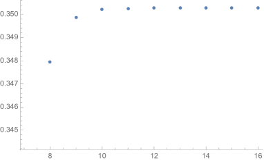
Figure 1: $f_{k}(\theta_{k})$

References

- [1] P.-A. Absil, R. Mahony and B. Andrews. Convergence of iterates of descent methods for analytic cost functions. SIAM J. Optim., vol. 16, no. 2, pp. 531-547, 2006.
- [2] S. Arimoto. An algorithm for computing the capacity of arbitrary memoryless channels. IEEE Trans. Info. Theory, vol. 18, no. 1, pp. 14-20, 1972.
- [3] D. P. Bertsekas. Nonlinear Programming, 2nd ed., Athena Scientific, Belmont, Massachusetts, 1999.
- [4] R. E. Blahut. Computation of channel capacity and rate distortion functions. IEEE Trans. Info. Theory, vol. 18, no. 4, pp. 460-473, 1972.
- [5] S. Boyd and L. Vandenberghe. Convex Optimization, Cambridge University Press, New York, 2004.
- [6] J. Chen and P. H. Siegel. Markov processes asymptotically achieve the capacity of finite-state intersymbol interference channels. IEEE Trans. Info. Theory, vol. 54, no. 3, pp. 1295-1303, 2008.
- [7] T. Cover and J. Thomas, Elements of Information Theory, 2nd ed., New York, NY: John Wiley & Sons, Jul. 2006.
- [8] G. D. Forney. Maximum likelihood sequence estimation of digital sequences in the presence of inter-symbol interference. IEEE Trans. Info. Theory, vol. 18, no. 3, pp. 363-378, 1972.
- [9] R. Gallager. Information Theory and Reliable Communication, Wiley, New York, 1968.
- [10] R. M. Gray. Entropy and Information Theory, Springer US, 2011.
- [11] G. Han. Limit theorems in hidden Markov models. IEEE Trans. Info. Theory, vol. 59, no. 3, pp. 1311-1328, 2013.
- [12] G. Han. A randomized algorithm for the capacity of finite-state channels. IEEE Trans. Info. Theory, vol. 61, no. 7, pp. 3651-3669, 2015.
- [13] G. Han and B. Marcus. Analyticity of entropy rate of hidden Markov chains. IEEE Trans. Info. Theory, vol. 52, no. 12, pp. 5251-5266, 2006.
- [14] G. Han and B. Marcus. Concavity of the mutual information rate for input-restricted memoryless channels at high SNR. IEEE Trans. Info. Theory, vol. 58, no. 3, pp. 1534-1548, 2012.
- [15] A. Kavčić. On the capacity of Markov sources over noisy channels. In Proc. IEEE Global Telecom. Conf., pp. 2997-3001, San Antonio, Texas, USA, Nov. 2001.
- [16] Y. Li and G. Han. Concavity of mutual information rate of finite-state channels. IEEE ISIT, pp. 2114-2118, 2013.
- [17] Y. Li and G. Han. Asymptotics of input-constrained erasure channel capacity. IEEE Trans. Info. Theory, vol. 64, no. 1, pp. 148-162, 2018.
- [18] Y. Li, G. Han and P. H. Siegel. On NAND flash memory channels with intercell interference. Work in progress.
- [19] D. Lind and B. Marcus. An Introduction to Symbolic Dynamics and Coding, Cambridge University Press, 1995.
- [20] B. Marcus, R. Roth and P. H. Siegel. Constrained systems and coding for recording channels. Handbook of Coding Theory, Elsevier Science, 1998.
- [21] M. Mushkin and I. Bar-David. Capacity and coding for the Gilbert-Elliott channel. IEEE Trans. Info. Theory, vol. 5, no. 6, pp. 1277-1290, 1989.
- [22] J. Proakis. Digital Communications, 4th ed., McGraw-Hill, New York, 2000.
- [23] H. Thapar and A. Patel. A class of partial response systems for increasing storage density in magnetic recording. IEEE Trans. Magn., vol. 23, no. 5, pp. 3666-3668, 1987.
- [24] P. O. Vontobel, A. Kavcic, D. Arnold and H.-A. Loeliger. A generalization of the Blahut-Arimoto algorithm to finite-state channels. IEEE Trans. Info. Theory, vol. 54, no. 5, pp. 1887-1918, 2008.
- [25] Chengyu Wu, Guangyue Han and Brian Marcus. A Deterministic Algorithm for the Capacity of Finite-State Channels, the 2019 IEEE International Symposium on Information Theory (ISIT), Paris, France, 2019.07.07-07.12