Is it Time to Swish?
Comparing Deep Learning Activation Functions Across NLP tasks
Abstract
Activation functions play a crucial role in neural networks because they are the non-linearities which have been attributed to the success story of deep learning. One of the currently most popular activation functions is ReLU, but several competitors have recently been proposed or ‘discovered’, including LReLU functions and swish. While most works compare newly proposed activation functions on few tasks (usually from image classification) and against few competitors (usually ReLU), we perform the first large-scale comparison of 21 activation functions across eight different NLP tasks. We find that a largely unknown activation function performs most stably across all tasks, the so-called penalized tanh function. We also show that it can successfully replace the sigmoid and tanh gates in LSTM cells, leading to a 2 percentage point (pp) improvement over the standard choices on a challenging NLP task.
1 Introduction
Activation functions are a crucial component of neural networks because they turn an otherwise linear classifier into a non-linear one, which has proven key to the high performances witnessed across a wide range of tasks in recent years. While different activation functions such as sigmoid or tanh are often equivalent on a theoretical level, in the sense that they can all approximate arbitrary continuous functions Hornik (1991), different activation functions often show very diverse behavior in practice.
For example, sigmoid, one of the activation functions dominating in neural network practice for several decades eventually turned out less suitable for learning because (according to accepted wisdom) of its small derivative which may lead to vanishing gradients. In this respect, the so-called ReLU function Glorot et al. (2011) has proven much more suitable. It has an identity derivative in the positive region and is thus claimed to be less susceptible to vanishing gradients. It has therefore (arguably) become the most popular activation function. The recognition of ReLU’s success has led to various extensions proposed Maas et al. (2013); He et al. (2015); Klambauer et al. (2017), but none has reached the same popularity, most likely because of ReLU’s simplicity and because the gains reported tended to be inconsistent or marginal across datasets and models Ramachandran et al. (2017).
Activation functions have been characterized by a variety of properties deemed important for successful learning, such as ones relating to their derivatives, monotonicity, and whether their range is finite or not. However, in recent work, Ramachandran et al. (2017) employed automatic search to find high-performing novel activation functions, where their search space contained compositions of elementary unary and binary functions such as , , , , or . They found many functions violating properties deemed as useful, such as non-monotonic activation functions or functions violating the gradient-preserving property of ReLU. Indeed, their most successful function, which they call swish, violates both of these conditions. However, as with previous works, they also only evaluated their newly discovered as well as their (rectifier) baseline activation functions on few different datasets, usually taken from the image classification community such as CIFAR Krizhevsky (2009) and ImageNet Russakovsky et al. (2015), and using few types of different networks, such as the deep convolutional networks abounding in the image classification community Szegedy et al. (2016).
To our best knowledge, there exists no large-scale empirical comparison of different activations across a variety of tasks and network architectures, and even less so within natural language processing (NLP).111An exception may be considered Xu et al. (2015), who, however, only contrast the rectifier functions on image classification datasets. Thus, the question which activation function really performs best and most stably across different NLP tasks and popular NLP models remains unanswered to this date.
In this work, we fill this gap. We compare (i) 21 different activation functions, including the 6 top performers found from automatic search in Ramachandran et al. (2017), across (ii) three popular NLP task types (sentence classification, document classification, sequence tagging) comprising 8 individual tasks, (iii) using three different popular NLP architectures, namely, MLPs, CNNs, and RNNs. We also (iv) compare all functions across two different dimensions, namely: top vs. average performance.
We find that a largely unknown activation function, penalized tanh Xu et al. (2016), performs most stably across our different tasks. We also find that it can successfully replace tanh and sigmoid activations in LSTM cells. We further find that the majority of top performing functions found in Ramachandran et al. (2017) do not perform well for our tasks. An exception is swish, which performed well across several tasks, but less stably than penalized tanh and other functions.222Accompanying code to reproduce our experiments is available from https://github.com/UKPLab/emnlp2018-activation-functions.
2 Theory
Activation functions
We consider 21 activation functions, 6 of which are “novel” and proposed in Ramachandran et al. (2017). The functional form of these 6 is given in Table 1, together with the sigmoid function.
| sigmoid | |
|---|---|
| swish | |
| maxsig | |
| cosid | |
| minsin | |
| arctid | |
| maxtanh | |
| lrelu-0.01 | |
| lrelu-0.30 | |
| penalized tanh |
The remaining 14 are: tanh, sin, relu, lrelu-0.01, lrelu-0.30, maxout-2, maxout-3, maxout-4, prelu, linear, elu, cube, penalized tanh, selu. We briefly describe them: lrelu-0.01 and lrelu-0.30 are the so-called leaky relu (LReLU) functions Maas et al. (2013); the idea behind them is to avoid zero activations/derivatives in the negative region of relu. Their functional form is given in Table 1. prelu He et al. (2015) generalizes the LReLU functions by allowing the slope in the negative region to be a learnable parameter. The maxout functions Goodfellow et al. (2013) are different in that they introduce additional parameters and do not operate on a single scalar input. For example, maxout-2 is the operation that takes the maximum of two inputs: , so the number of learnable parameters is doubled. maxout-3 is the analogous function that takes the maximum of three inputs. As shown in Goodfellow et al. (2013), maxout can approximate any convex function. sin is the standard sine function, proposed in neural network learning, e.g., in Parascandolo et al. (2016), where it was shown to enable faster learning on certain tasks than more established functions. penalized tanh Xu et al. (2016) has been defined in analogy to the LReLU functions, which can be thought of as “penalizing” the identity function in the negative region. The reported good performance of penalized tanh on CIFAR-100 Krizhevsky (2009) lets the authors speculate that the slope of activation functions near the origin may be crucial for learning. linear is the identity function, . cube is the function , proposed in Chen and Manning (2014) for an MLP used in dependency parsing. elu Clevert et al. (2015) has been proposed as (yet another) variant of relu that assumes negative values, making the mean activations more zero-centered. selu is a scaled variant of elu used in Klambauer et al. (2017) in the context of so-called self-normalizing neural nets.
Properties of activation functions
| Property | Description | Problems | Examples |
|---|---|---|---|
| derivative | exploding gradient (e) | sigmoid (v), tanh (v), cube (e) | |
| vanishing (v) | |||
| zero-centered | range centered around zero? | if not, slower learning | tanh (), relu () |
| saturating | finite limits | vanishing gradient in the limit | tanh, penalized tanh, sigmoid |
| monotonicity | unclear | exceptions: sin, swish, minsin |
.
Many properties of activation functions have been speculated to be crucial for successful learning. Some of these are listed in Table 2, together with brief descriptions and illustrations.
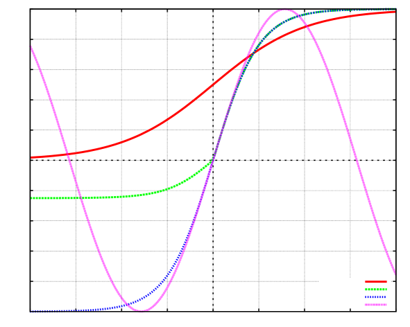
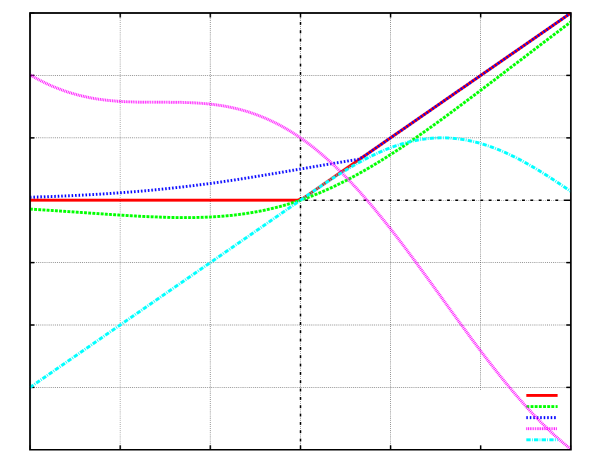
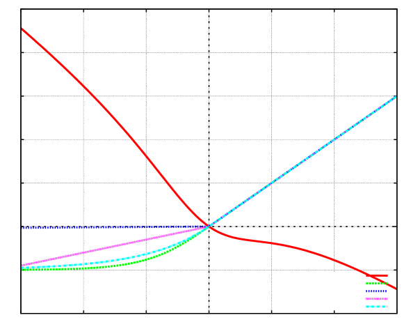
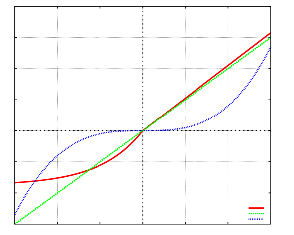
Graphs of all activation functions can be found in the appendix.
3 Experiments
We conduct experiments using three neural network types and three types of NLP tasks, described in §3.1, §3.2, and §3.3 below.
3.1 MLP & Sentence Classification
Model
We experiment with a multi-layer perceptron (MLP) applied to sentence-level classification tasks. That is, input to the MLP is a sentence or short text, represented as a fixed-size vector embedding. The output of the MLP is a label which classifies the sentence or short text. We use two sentence representation techniques, namely, Sent2Vec Pagliardini et al. (2018), of dimensionality 600, and InferSent Conneau et al. (2017), of dimensionality 4096. Our MLP has the form:
where is the input representation, are hidden layer representations, and is the output, a probability distribution over the classes in the classification task. Vectors and matrices are the learnable parameters of our network. The activation function is given by and ranges over the choices described in §2.
Data
We use four sentence classification tasks, namely: movie review classification (MR), subjectivitiy classification (SUBJ), question type classification (TREC), and classifying whether a sentence contains an argumentation structure of a certain type (claim, premise, major claim) or else is non-argumentative (AM). The first three datasets are standard sentence classification datasets and contained in the SentEval framework.333https://github.com/facebookresearch/SentEval We choose the AM dataset for task diversity, and derive it by projecting token-level annotations in the dataset from Stab and Gurevych (2017) to the sentence level. In the rare case (5% of the cases) when a sentence contains multiple argument types, we choose one based on the ordering Major Claim (MC) Claim (C) Premise (P). Datasets and examples are listed in Table 3.
| Task | Type | Size | C | Example |
| AM | Argumentation | 7k | 4 | Not cooking fresh food will lead to lack of nutrition. (claim) |
| MR | Sentiment | 11k | 2 | Too slow for a younger crowd , too shallow for an older one. (neg) |
| SUBJ | Subjectivity | 10k | 2 | A movie that doesn’t aim too high , but doesn’t need to. (subj) |
| TREC | Question-types | 6k | 6 | What’s the Olympic Motto? (description) |
| NG | Doc classification | 18k | 20 | […] You can add ”dark matter” and quarks […] (sci.space) |
| R8 | Doc classification | 7k | 8 | bowater industries profit exceed […] (earn) |
| POS | POS tagging | 204k | 17 | What/PRON to/PART feed/VERB my/PRON dog/NOUN […] |
| TL-AM | Token-level AM | 148k | 7 | […] I/O firmly/O believe/O that/O we/B-MC should/I-MC […] |
Approach
We consider 7 “mini-experiments”:
-
•
(1): MR dataset with Sent2Vec-unigram embeddings as input and 1% of the full data as training data; (2): the same mini-experiment with 50% of the full data as training data. In both cases, the dev set comprises 10% of the full data and the rest is for testing.
-
•
(3,4): SUBJ with InferSent embeddings and likewise 1% and 50% of the full data as train data, respectively.
-
•
(5): The TREC dataset with original split in train and test; 50% of the train split is used as dev data.
-
•
(6): The AM dataset with original split in train, dev, and test Eger et al. (2017), and with InferSent input embeddings. (7): the same mini-experiment with Sent2Vec-unigram embeddings.
We report accuracy for mini-experiments (1-5) and macro-F1 for (6-7). We report macro-F1 for (6-7) because the AM dataset is imbalanced.
The motivation behind choosing different input embeddings for different tasks was to investigate a wider variety of conditions. Choosing subsets of the full data had the same intention.
For all 7 mini-experiments, we draw the same 200 randomly chosen hyperparameters from the ranges indicated in Table 4. All experiments are conducted in keras.444https://keras.io/
For each of the 21 different activation functions detailed in §2, we conduct each mini-experiment with the 200 randomly chosen hyperparameters. All activation functions use the same hyperparameters and the same train, dev, and test splits.
We store two results for each mini-experiment, namely: (i) the test result corresponding to the best (best) dev performance; (ii) the average (mean) test result across all hyperparameters. The best result scenario mirrors standard optimization in machine learning: it indicates the score one can obtain with an activation function when the MLP is well-optimized. The mean result scenario is an indicator for what one can expect when hyperparameter optimization is ‘shallow’ (e.g., because computing times are prohibitive): it gives the average performance for randomly chosen hyperparameters. We note that we run each hyperparameter combination with 5 different random weight initializations and all the reported scores (best dev score, best best, best mean) are averages over these 5 random initializations.
Finally, we set the following hyperparameters for all MLP experiments: patience of 10 for early stopping, batch size 16, 100 epochs for training.
| Model | Hyperparameter | Range |
| (a) MLP | (1) optimizer | Adam,RMSprop,Adagrad,Adadelta,Adamax,Nadam,sgd |
| (2) #hidden layers | ||
| (3) dropout value | ||
| (4) hidden units | ||
| (5) learning rate | ||
| (6) weight initializer | random-n, random-u, varscaling, orthogonal, | |
| lecun-u, glorot-n, glorot-u, he-n, he-u | ||
| (b) CNN | (a) (1,3,5,6) | same as MLP |
| embedding dimension | ||
| number of filters | ||
| #hidden layers | ||
| filter size | ||
| (c) RNN/LSTM | (a) (1-5) | same as MLP |
| recurrent initializer | same as (a) (6) plus identity matrix |
Results
Figure 1 shows best and mean results, averaged over all 7 mini-experiments, for each activation function. To make individual scores comparable across mini-experiments, we perform max normalization and divide each score by the maximum score achieved in any given mini-experiment (for best and mean, respectively) before averaging.555We chose max normalization so that certain tasks/mini-experiments would not unduly dominate our averaged scores. Overall, our averaged scores are not (much) affected by this decision, however: the Spearman correlation of rankings of activation functions under max normalization and under no max normalization are above 0.98 in all our three classification scenarios considered in §3.1,§3.2,§3.3.
For best, the top performers are the rectifier functions (relu, lrelu-0.01, prelu) as well as maxout and penalized tanh. The newly discovered activation functions lag behind, with the best of them being minsin and swish. linear is worst, together with elu and cube. Overall, the difference between the best activation function, relu, and the worst, linear, is only roughly 2pp, however. This means that if hyperparameter search is done carefully, the choice of activation function is less important for these sentence classification tasks. Particularly the (binary) tasks MR and SUBJ appear robust against the choice of activation function, with the difference between the best and worst function being always less than 1pp, in all settings. For TREC and AM, the situation is slightly different: for TREC, the difference is 2pp (swish vs. maxsig) and for AM, it is 3pp using InferSent embeddings (swish vs. cube) and 12pp using Sent2Vec embeddings (relu vs. linear). It is noteworthy that swish wins 2 out of 3 cases in which the choice of activation function really matters.
mean results are very different from best results. Here, somewhat surprisingly, the oscillating sin function wins, followed by penalized tanh, maxout and swish. The difference between the best mean function, sin, and the worst, cube, is more than 30pp. This means that using cube is much riskier and requires more careful hyperparameter search compared to sin and the other top performers.
3.2 CNN & Document Classification
Model
Our second paradigm is document classification using a CNN. This approach has been popularized in NLP by the ground-breaking work of Kim (2014). Even though shallow CNNs do not reach state-of-the-art results on large datasets anymore Johnson and Zhang (2017), simple approaches like (shallow) CNNs are still very competitive for smaller datasets Joulin et al. (2016).
Our model operates on token-level and first embeds a sequence of tokens , represented as 1-hot vectors, into learnable embeddings . The model then applies 1D-convolution on top of these embeddings. That is, a filter of size takes successive embeddings , performs a scalar product and obtains a feature :
Here, is the activation function and is a bias term. We take the number of different filters as a hyperparameter. When our network has multiple layers, we stack another convolutional layer on top of the first (in total we have outputs at each time step), and so on. Our penultimate layer is a global max pooling layers that selects the maximum from each feature map. A final softmax layer terminates the network.
Data
We use two document classification tasks, namely: 20 Newsgroup (NG) and Reuters-21578 R8 (R8). Both datasets are standard document classification datasets. In NG, the goal is to classify each document into one of 20 newsgroup classes (alt.atheism, sci.med, sci.space, etc.). In R8, the goal is to classify Reuters news text into one of eight classes (crude, earn, grain, interest, etc.). We used the preprocessed files from https://www.cs.umb.edu/~smimarog/textmining/datasets/ (in particular, stopwords are removed and the text is stemmed).
Approach
We consider 4 mini-experiments:
-
•
(1,2) NG dataset with 5% and 50%, respectively of the full data as train data. In both cases, 10% of the full data is used as dev data, and the rest as test data.
-
•
(3,4) Same as (1,2) for R8.
We report accuracy for all experiments. We use a batch size of 64, 50 epochs for training, and a patience of 10. For all mini-experiments, we again draw 200 randomly chosen hyperparameters from the ranges indicated in Table 4. The hyperparameters and train/dev/test splits are the same for all activation functions.
Results
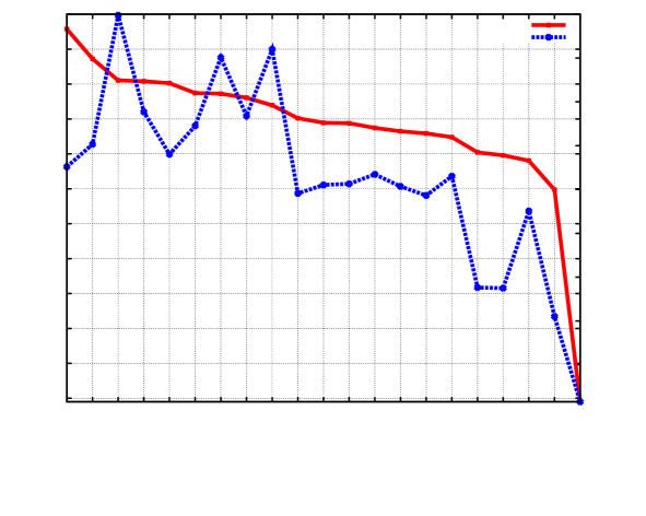
Figure 2 shows best and mean results, averaged over all mini-experiments. This time, the winners for best are elu, selu (again two members from the rectifier family), and maxout-3, but the difference between maxout-3 and several lower ranked functions is minimal. The cube function is again worst and sigmoid and cosid have similarly bad performance. Except for minsin, the newly proposed activation functions from Ramachandran et al. (2017) again considerably lag behind. The most stable activation functions are the maxout functions as well as penalized tanh, tanh and sin.
3.3 RNN & Sequence Tagging
Model
Our third paradigm is sequence tagging, a ubiquitous model type in NLP. In sequence tagging, a sequence of input tokens is mapped to a sequence of labels . Classical sequence tagging tasks include POS tagging, chunking, NER, discourse parsing Braud et al. (2017), and argumentation mining Eger et al. (2017); Schulz et al. (2018). We use a standard recurrent net for sequence tagging, whose form is:
Here, are (pre-trained) word embeddings of words . Vectors and matrices are parameters to be learned during training. The above describes an RNN with only one hidden layer, , at each time step, but we consider the generalized form with hidden layers; we also choose a bidirectional RNN in which the hidden outputs of a forward RNN and a backward RNN are combined. RNNs are particularly deep networks—indeed, the depth of the network corresponds to the length of the input sequence—which makes them particularly susceptible to the vanishing gradient problem Pascanu et al. (2012).
Initially, we do not consider the more popular LSTMs here for reasons indicated below. However, we include a comparison after discussing the RNN performance.
Data
We use two sequence tagging tasks, namely: English POS tagging (POS), and token-level argumentation mining (TL-AM) using the same dataset (consisting of student essays) as for the sentence level experiments. In token-level AM, we tag each token with a BIO-label plus the component type, i.e., the label space is , where ‘O” is a label for non-argumentative tokens. The motivation for using TL-AM is that, putatively, AM has more long-range dependencies than POS or similar sequence tagging tasks such as NER, because argument components are much longer than named entities and component labels also depend less on the current token.
Approach
We consider 6 mini-experiments:
-
•
(1): TL-AM with Glove-100d word embeddings and 5% of the original training data as train data; (2) the same with 30% of the original training data as train data. In both cases, dev and test follow the original train splits Eger et al. (2017).
-
•
(3,4) Same as (1) and (2) but with 300d Levy word embeddings Levy and Goldberg (2014).
-
•
(5,6): POS with Glove-100d word embeddings and 5% and 30%, respectively, of the train data of a pre-determined train/dev/test split (13k/13k/178k tokens). Dev and test are fixed in both cases.
We report macro-F1 for mini-experiments (1-4) and accuracy for (5-6). For our RNN implementations, we use the accompanying code of (the state-of-the-art model of) Reimers and Gurevych (2017), which is implemented in keras. The network uses a CRF layer as an output layer. We use a batch size of 32, train for 50 epochs and use a patience of 5 for early stopping.
Results
Figure 3 shows best and mean results, averaged over all 6 mini-experiments, for each activation function. We exclude prelu and the maxout functions because the keras implementation does not natively support these activation functions for RNNs. We also exclude the cube function because it performed very badly.
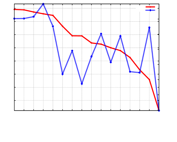
Unlike for sentence classification, there are much larger differences between the activation functions. For example, there is almost 20pp difference between the best best activation functions: relu, lrelu-0.01, swish, penalized tanh, and the worst ones: linear, cosid, and sigmoid (the differences were larger had we included cube). Interestingly, this difference is mostly due to the TL-AM task: for POS, there is only 3pp difference between the best function (sigmoid (sic!), though with almost zero margin to the next best ones) and the worst one (linear), while this difference is almost 40pp for TL-AM. This appears to confirm our concerns regarding the POS tagging task as not being challenging enough due to lack of, e.g., long-range dependencies.
The four best best activation functions in Figure 3 are also the functions with the best mean results, i.e., they are most stable over different hyperparameters. The clear winner in this category is penalized tanh with 100% mean score, followed by swish with 91%. Worst is cosid with 30%. It is remarkable how large the difference between tanh and penalized tanh is both for best and mean—7pp and 20pp, respectively, which is much larger than the differences between the analogous pair of LReLU and relu. This appears to make a strong case for the importance of the slope around the origin, as suggested in Xu et al. (2016).
LSTM vs. RNN
Besides an RNN, we also implemented a more popular RNN model with (bidirectional) LSTM blocks in place of standard hidden layers. Standard LSTM units follow the equations (simplified):
where and are perceived of as gates that control information flow, is the input at time and is the hidden layer activation. In keras (and most standard references), is the (hard) sigmoid function, and is the tanh function.
We ran an LSTM on the TL-AM dataset with Levy word embeddings and 5% and 30% data size setup. We varied and independently, keeping the respective other function at its default.
We find that the top two choices for are penalized tanh and tanh (margin of 10pp), given that is sigmoid. For tanh, the best choices are penalized tanh, sigmoid, and tanh. All other functions perform considerably worse. Thus, the top-performers are all saturating functions, indicating the different roles activation functions play in LSTMs—those of gates—compared to standard layers. It is worth mentioning that choosing or as penalized tanh is on average better than the standard choices for and . Indeed, choosing penalized tanh is on average 2pp better than the default choices of .
It is further worth mentioning that the best best results for the LSTM are roughly 5pp better (absolute) than the best corresponding choices for the simple RNN.
4 Analysis & Discussion
Winner statistics
Each of the three meta-tasks sentence classification, document classification, and sequence tagging was won, on average, by a member from the rectifier family, namely, relu (2) and elu, for best. Also, in each case, cube and cosid were among the worst performing activation functions. The majority of newly proposed functions from Ramachandran et al. (2017) ranked somewhere in the mid-field, with swish and minsin performing best in the best category. For the mean category, we particulary had the maxout functions as well as penalized tanh and sin regularly as top performers.
To get further insights, we computed a winner statistic across all 17 mini-experiments, counting how often each activation function was among the top 3. Table 5 shows the results, excluding prelu and the maxout functions because they were not considered in all mini-experiments.
| best | penalized tanh (6), swish (6), |
|---|---|
| elu (4), relu (4), lrelu-0.01 (4) | |
| mean | penalized tanh (16), tanh (13) |
| sin (10) |
We see that penalized tanh and swish win here for best, followed by further rectifier functions. The mean category is clearly won by saturating activation functions with finite range. If this comparison were restricted to sentence and document classification, where we also included the maxout functions, then penalized tanh would have been outperformed by maxout for mean.
This appears to yield the conclusion that functions with limited range behave more stably across hyperparameter settings while non-saturating functions tend to yield better top-performances. The noteworthy exception to this rule is penalized tanh which excels in both categories (the more expensive maxout functions would be further exceptions). If the slope around the origin of penalized tanh is responsible for its good performance, then this could also explain why cube is so bad, since it is very flat close to the origin.
Influence of hyperparameters
To get some intuition about how hyperparameters affect our different activation functions, we regressed the score of the functions on the test set on all the employed hyperparameters. For example, we estimated:
| (1) |
where is the score on the test set, is the number of layers in the network, is the dropout value, etc. The coefficients for each regressor is what we want to estimate (in particular, their size and their sign). We logarithmized certain variables whose scale was substantially larger than those of others (e.g., number of units, number of filters). For discrete regressors such as the optimizer we used binary dummy variables. We estimated Eq. (1) independently for each activation function and for each mini-experiment. Overall, there was a very diverse pattern of outcomes, preventing us from making too strong conclusions. Still, we observed that while all models performed on average better with fewer hidden layers, particularly swish was robust to more hidden layers (small negative coefficient ), but also, to a lesser degree, penalized tanh. In the sentence classification tasks, sin and the maxout functions were particulary robust to an increase of hidden layers. Since penalized tanh is a saturating function and sin even an oscillating one, we therefore conclude that preserving the gradient (derivative close to one) is not a necessary prerequisite to successful learning in deeper neural networks.
5 Concluding remarks
We have conducted the first large scale comparison of activation functions across several different NLP tasks (and task types) and using different popular neural network types. Our main focus was on so-called scalar activation functions, but we also partly included the more costly ‘many-to-one’ maxout functions.
Our findings suggest that the rectifier functions (and the similarly shaped swish) can be top performers for each task, but their performance is unstable and cannot be predicted a priori. One of our major findings is that, in contrast, the saturating penalized tanh function performs much more stably in this respect and can with high probability be expected to perform well across tasks as well as different choices of hyperparameters. This appears to make it the method of choice particularly when hyperparameter optimization is costly. When hyperparameter optimization is cheap, we recommend to consider the activation function as another hyperparameter and choose it, e.g., from the range of functions listed in Table 5 along with maxout.
Another major advantage of the penalized tanh function is that it may also take the role of a gate (because of its finite range) and thus be employed in more sophisticated neural network units such as LSTMs, where the rectifiers fail completely. In this context, we noticed that replacing sigmoid and tanh in an LSTM cell with penalized tanh leads to a 2pp increase on a challenging NLP sequence tagging task. Exploring whether this holds across more NLP tasks should be scope for future work. Additionally, our research suggests it is worthwhile to further explore penalized tanh, an arguably marginally known activation function. For instance, other scaling factors than (default value from Xu et al. (2016)) should be explored. Similarly as for prelu, the scaling factor can also be made part of the optimization problem.
Finally, we found that except for swish none of the newly discovered activation functions found in Ramachandran et al. (2017) made it in our top categories, suggesting that automatic search of activation functions should be made across multiple tasks in the future.
Acknowledgments
We thank Teresa Bötschen, Nils Reimers and the anonymous reviewers for helpful comments. This work has been supported by the German Federal Ministry of Education and Research (BMBF) under the promotional reference 01UG1816B (CEDIFOR).
References
- Braud et al. (2017) Chloé Braud, Ophélie Lacroix, and Anders Søgaard. 2017. Cross-lingual and cross-domain discourse segmentation of entire documents. In Proceedings of the 55th Annual Meeting of the Association for Computational Linguistics, volume 2, pages 237–243.
- Chen and Manning (2014) Danqi Chen and Christopher Manning. 2014. A fast and accurate dependency parser using neural networks. In Proceedings of the 2014 Conference on Empirical Methods in Natural Language Processing (EMNLP), pages 740–750, Doha, Qatar. Association for Computational Linguistics.
- Clevert et al. (2015) Djork-Arné Clevert, Thomas Unterthiner, and Sepp Hochreiter. 2015. Fast and accurate deep network learning by exponential linear units (elus). CoRR, abs/1511.07289.
- Conneau et al. (2017) Alexis Conneau, Douwe Kiela, Holger Schwenk, Loic Barrault, and Antoine Bordes. 2017. Supervised Learning of Universal Sentence Representations from Natural Language Inference Data. In Proceedings of the 2017 Conference on Empirical Methods in Natural Language Processing (EMNLP 2017), pages 681–691. Association for Computational Linguistics.
- Eger et al. (2017) Steffen Eger, Johannes Daxenberger, and Iryna Gurevych. 2017. Neural end-to-end learning for computational argumentation mining. In Proceedings of the 55th Annual Meeting of the Association for Computational Linguistics (Volume 1: Long Papers), pages 11–22, Vancouver, Canada. Association for Computational Linguistics.
- Glorot et al. (2011) Xavier Glorot, Antoine Bordes, and Yoshua Bengio. 2011. Deep sparse rectifier neural networks. In Proceedings of the Fourteenth International Conference on Artificial Intelligence and Statistics, volume 15 of Proceedings of Machine Learning Research, pages 315–323, Fort Lauderdale, FL, USA. PMLR.
- Goodfellow et al. (2013) Ian J. Goodfellow, David Warde-Farley, Mehdi Mirza, Aaron Courville, and Yoshua Bengio. 2013. Maxout networks. In Proceedings of the 30th International Conference on International Conference on Machine Learning - Volume 28, ICML’13, pages III–1319–III–1327. JMLR.org.
- He et al. (2015) Kaiming He, Xiangyu Zhang, Shaoqing Ren, and Jian Sun. 2015. Delving deep into rectifiers: Surpassing human-level performance on imagenet classification. In Proceedings of the 2015 IEEE International Conference on Computer Vision (ICCV), ICCV ’15, pages 1026–1034, Washington, DC, USA. IEEE Computer Society.
- Hornik (1991) Kurt Hornik. 1991. Approximation capabilities of multilayer feedforward networks. Neural Netw., 4(2):251–257.
- Johnson and Zhang (2017) Rie Johnson and Tong Zhang. 2017. Deep pyramid convolutional neural networks for text categorization. In Proceedings of the 55th Annual Meeting of the Association for Computational Linguistics (Volume 1: Long Papers), volume 1, pages 562–570.
- Joulin et al. (2016) Armand Joulin, Edouard Grave, Piotr Bojanowski, and Tomas Mikolov. 2016. Bag of tricks for efficient text classification. CoRR, abs/1607.01759.
- Kim (2014) Yoon Kim. 2014. Convolutional neural networks for sentence classification. In Proceedings of the 2014 Conference on Empirical Methods in Natural Language Processing (EMNLP), pages 1746–1751. Association for Computational Linguistics.
- Klambauer et al. (2017) Günter Klambauer, Thomas Unterthiner, Andreas Mayr, and Sepp Hochreiter. 2017. Self-normalizing neural networks. In I. Guyon, U. V. Luxburg, S. Bengio, H. Wallach, R. Fergus, S. Vishwanathan, and R. Garnett, editors, Advances in Neural Information Processing Systems 30, pages 971–980. Curran Associates, Inc.
- Krizhevsky (2009) A. Krizhevsky. 2009. Learning multiple layers of features from tiny images. Master’s thesis, Computer Science Department, University of Toronto.
- Levy and Goldberg (2014) Omer Levy and Yoav Goldberg. 2014. Dependency-based word embeddings. In Proceedings of the 52nd Annual Meeting of the Association for Computational Linguistics (Volume 2: Short Papers), pages 302–308. Association for Computational Linguistics.
- Maas et al. (2013) Andrew L. Maas, Awni Y. Hannun, and Andrew Y. Ng. 2013. Rectifier nonlinearities improve neural network acoustic models. In International Conference on Machine Learning (ICML).
- Pagliardini et al. (2018) Matteo Pagliardini, Prakhar Gupta, and Martin Jaggi. 2018. Unsupervised Learning of Sentence Embeddings using Compositional n-Gram Features. In NAACL 2018 - Conference of the North American Chapter of the Association for Computational Linguistics.
- Parascandolo et al. (2016) Giambattista Parascandolo, Heikki Huttunen, and Tuomas Virtanen. 2016. Taming the waves: sine as activation function in deep neural networks.
- Pascanu et al. (2012) Razvan Pascanu, Tomas Mikolov, and Yoshua Bengio. 2012. Understanding the exploding gradient problem. CoRR, abs/1211.5063.
- Ramachandran et al. (2017) Prajit Ramachandran, Barret Zoph, and Quoc V. Le. 2017. Searching for activation functions. CoRR, abs/1710.05941.
- Reimers and Gurevych (2017) Nils Reimers and Iryna Gurevych. 2017. Reporting Score Distributions Makes a Difference: Performance Study of LSTM-networks for Sequence Tagging. In Proceedings of the 2017 Conference on Empirical Methods in Natural Language Processing (EMNLP), pages 338–348, Copenhagen, Denmark.
- Russakovsky et al. (2015) Olga Russakovsky, Jia Deng, Hao Su, Jonathan Krause, Sanjeev Satheesh, Sean Ma, Zhiheng Huang, Andrej Karpathy, Aditya Khosla, Michael Bernstein, Alexander C. Berg, and Li Fei-Fei. 2015. Imagenet large scale visual recognition challenge. Int. J. Comput. Vision, 115(3):211–252.
- Schulz et al. (2018) Claudia Schulz, Steffen Eger, Johannes Daxenberger, Tobias Kahse, and Iryna Gurevych. 2018. Multi-task learning for argumentation mining in low-resource settings. In Proceedings of the 16th Annual Conference of the North American Chapter of the Association for Computational Linguistics: Human Language Technologies, page to appear. Association for Computational Linguistics.
- Stab and Gurevych (2017) Christian Stab and Iryna Gurevych. 2017. Parsing argumentation structures in persuasive essays. Computational Linguistics, 43(3):619–659.
- Szegedy et al. (2016) Christian Szegedy, Sergey Ioffe, and Vincent Vanhoucke. 2016. Inception-v4, inception-resnet and the impact of residual connections on learning. CoRR, abs/1602.07261.
- Xu et al. (2016) Bing Xu, Ruitong Huang, and Mu Li. 2016. Revise saturated activation functions. CoRR, abs/1602.05980.
- Xu et al. (2015) Bing Xu, Naiyan Wang, Tianqi Chen, and Mu Li. 2015. Empirical evaluation of rectified activations in convolutional network. CoRR, abs/1505.00853.
Appendix A Supplemental Material
