Discovery, observations and modelling of a new eclipsing polar: MASTER OT J061451.70–272535.5

Abstract

We report the discovery of a new eclipsing polar, MASTER OT J061451.70–272535.5, detected as an optical transient by MASTER auto-detection software at the recently commissioned MASTER-SAAO telescope. Time resolved (10–20 s) photometry with the SAAO 1.9-m, and 1.0-m telescopes, utilizing the SHOC EM-CCD cameras, revealed that the source eclipses, with a period of 2.08 hours (7482.9$\pm$3.5 s). The eclipse light curve has a peculiar morphology, comprising an initial dip, where the source brightness drops to $\sim$50% of the pre-eclipse level before gradually increasing again in brightness. A second rapid ingress follows, where the brightness drops by $\sim$60–80%, followed by a more gradual decrease to zero flux. We interpret the eclipse profile as the result of an initial obscuration of the accretion hot-spot on the magnetic white dwarf by the accretion stream, followed by an eclipse of both the hot-spot and the partially illuminated stream by the red dwarf donor star. This is similar to what has been observed in other eclipsing polars such as HU Aqr, but here the stream absorption is more pronounced. The object was subsequently observed with South African Large Telescope (SALT) using the Robert Stobie Spectrograph (RSS). This revealed a spectrum with all of the Balmer lines in emission, a strong He ii 4686 Å line with a peak flux greater than that of H$\beta$, as well as weaker He i lines. The spectral features, along with the structure of the light curve, suggest MASTER OT J061451.70–272535.5 is a new magnetic cataclysmic variable, most likely of the synchronised Polar subclass.

1 Introduction

Magnetic cataclysmic variables (mCVs) are close binary stars consisting of a magnetic white dwarf (WD) accreting from a low mass M or K dwarf companion (Warner, 2003; Hellier, 2001). The sub-class of mCVs known as polars (Cropper, 1990), or sometimes AM Herculis stars, have white dwarfs whose rotation is synchronised (or nearly synchronised), to the orbital period. MCVs are significant accretion-driven X-ray sources, with luminosities in the range of $L_{X}\sim 10^{31}-10^{32}$ erg s^-1, a fact which has lead to many of them being discovered by X-ray surveys (see for example Rojas et al. (2017), Masetti et al. (2013) and associated articles). In polars, the strength of the white dwarf’s magnetic field, coupled with the short orbital period – and therefore close proximity of the two stars – leads to accreted material from the inner Lagrangian point, L1, being injected near the magnetosphere of the primary. At some distance from the white dwarf, the magnetic force dominates over the ram pressure of the accreting material, preventing the formation of an accretion disk. Material then accretes along magnetic field lines, which funnel the plasma into an accretion column near the white dwarf’s magnetic pole. As material impacts the surface of the WD at supersonic velocities, a deceleration shock is produced in the flow at ${\sim}10^{4}$ m above the WD surface. In passing through the shock, the bulk kinetic motion of the gas becomes thermalised, producing a hot (${\sim}10^{8}$ K) settling flow in the post-shock region. Some polars accrete onto both poles (e.g. Beardmore et al., 1995; Schwope et al., 1995; Schmidt et al., 1999; O’Donoghue et al., 2006), while others are single pole accretors (e.g. Schwope et al., 1993; Salvi et al., 2002; Bridge et al., 2003), and some switch between single and multiple pole accretion as the mass transfer rate or the magnetic field geometry changes (e.g. Rosen et al., 1996; Mason et al., 1998; Denisenko & Martinelli, 2016).

The X-ray spectra of mCVs are typically characterised by two components, namely a hard ($kT>10$ keV) bremsstrahlung component and a soft ($kT\sim 20-50$ eV) pseudo-blackbody component. The former arises from bremsstrahlung emission in the post-shock accretion flow, just above the white dwarf surface. The latter is typically attributed to the result of reprocessing and/or direct bombardment due to a fragmented stream from which diamagnetic accretion “blobs” bury themselves in the photosphere of the white dwarf and re-radiate their kinetic energy (Beuermann, 2004). A resulting hot-spot is therefore produced near the magnetic poles which can often be seen in high time resolution eclipse light curves of polars (e.g. O’Donoghue et al. (2006)). These hot-spots are typically very small, ${\sim}10^{-4}$ of the surface area of the white dwarf, but can produce a significant fraction of the total luminosity of the system. See Mukai (2017) for a review of the X-ray properties of accreting WDs.

A defining characteristic of polars – as their name suggests – is the high level of optical polarization arising from cyclotron emission in the post-shock accretion flow, which can reach levels of ${\sim}50\%$ for circular polarization (Hakala et al., 1994). Magnetic field strengths in polars, which range from 7–230 MG (Ferrario et al., 2015b), have, for the most part, been determined by fitting models to spectro-polarimetric observations. In some cases, particularly when the accretion rate is low, magnetic field estimates can be made from measuring the Zeeman splitting of photospheric spectral lines (Beuermann et al., 2007). Another observational feature of polars is that their spectra typically show strong Balmer, He i and He ii emission lines, with the latter generally much stronger ($F_{H\beta}<F_{\text{He\,{ii}}}$) in polars and mCVs compared to non-magnetic cataclysmic variables (Szkody, 1998).

MCVs constitute a small fraction of the total number of known CVs (${\sim}15-25$%) – about half of these being polars, and the other half the lower field asynchronous Intermediate polars (IPs) (for a review of IPs, see Patterson (1994)). Of the 141 polars in the latest edition of the Ritter & Kolb catalogue of cataclysmic variables and related objects (v7.24, December 2015: Ritter & Kolb (2003)), 92% have periods $\leq$3.8 h, with the shortest period system at 48.6 minutes. The median period is 1.93 h, which means that slightly more than half of the known polars have periods below the ${\sim}2-3$ hour period gap. Figure 1 compares the orbital period distribution of polars and IPs. The surplus of the number of polars at shorter periods, as compared to that of the IPs, can readily be seen. Whether or not the reason for this is due to an evolutionary transition or selection effects, remains a matter of debate (Mason, 2004; Hong et al., 2012).

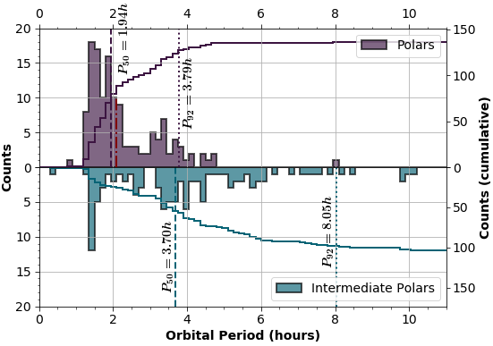
Figure 1: The orbital period distribution of the known mCVs at the time of publication using data from Ritter & Kolb (2003). The figure shows back-to-back histograms of the two classes of mCVs over the orbital period range of 0–11 hours. Also shown for each class are the cumulative histograms (solid, stepped lines), the median period $P_{50}$ (dashed vertical lines), and the 92 percentile period $P_{92}$ (dotted vertical lines). The surplus of polars at short periods is clearly seen – approximately 90% of polars have periods shorter than the median period for the IPs. For reference, the orbital period of J0614–27 (see subsection 4.1) is also indicated as the red dash-dotted vertical line at $P=2.078$ h in the upper panel.

At the time of writing there are 33 polars that have been positively identified as eclipsing systems, which makes the discovery of a new example an important addition. Eclipsing systems allow indirect mapping of the gas flow and accretion on to the white dwarf, since the positions and dimensions of the accretion regions (the “hot-spots”), the accretion stream and the interaction/threading region in the magnetosphere, can be determined by virtue of the secondary’s occulting limb (Hakala, 1995; Harrop-Allin et al., 1999; O’Donoghue et al., 2006). In a wider context, eclipsing polars are ideal cosmic laboratories for studying magnetic accretion, which occurs in many other astrophysical objects, including protostellar objects (e.g. T Tau stars), pulsars and active galactic nuclei.

Here we report on the discovery of a new eclipsing cataclysmic variable from the MASTER-SAAO optical transient survey, MASTER OT J061451.70–272535.5 (hereafter J0614–27). Follow-up time resolved photometry shows the system exhibits a deep, sharp eclipse, and a pre-eclipse “dip”, likely due to obscuration of the accretion spot(s) by the accretion stream. Spectroscopy from SALT reveals a spectrum characteristic of a polar, with the high-excitation emission line of He ii at 4686 Å, exceeding in flux that of H$\beta$ at 4861 Å, a standard hallmark of an mCV (Szkody, 1998).

2 The MASTER–SAAO facility and the discovery of J0614–27

2.1 MASTER–SAAO

Table 1: MASTER and CTRS survey parameter comparisons.

Parameter	CRTS	CRTS	MASTER	MASTER
	all nodes	SSS node	all nodes	SAAO node
Collecting area (m2)	2.35	0.20	1.50	0.25
Field of View (deg2)	13.3	4.0	64.0	8.0
Maximum area/night (deg2)	$\sim$2500:	unknown	$\sim$4000	$\sim$500–1000
Cadence (days)	7–10	7–10	10–15	10–20
Exposures (sec)	4 $\times$ 30	4 $\times$ 30	3 $\times$ (60–180)	3 $\times$ (60–180)∗
Limiting magnitude	19–20; 22#	19–20	18–20	19–20
Alert threshold (mags)	0.65	0.65	2.2	2.2
* depending on Moon phase
# limit for CSS node in USA

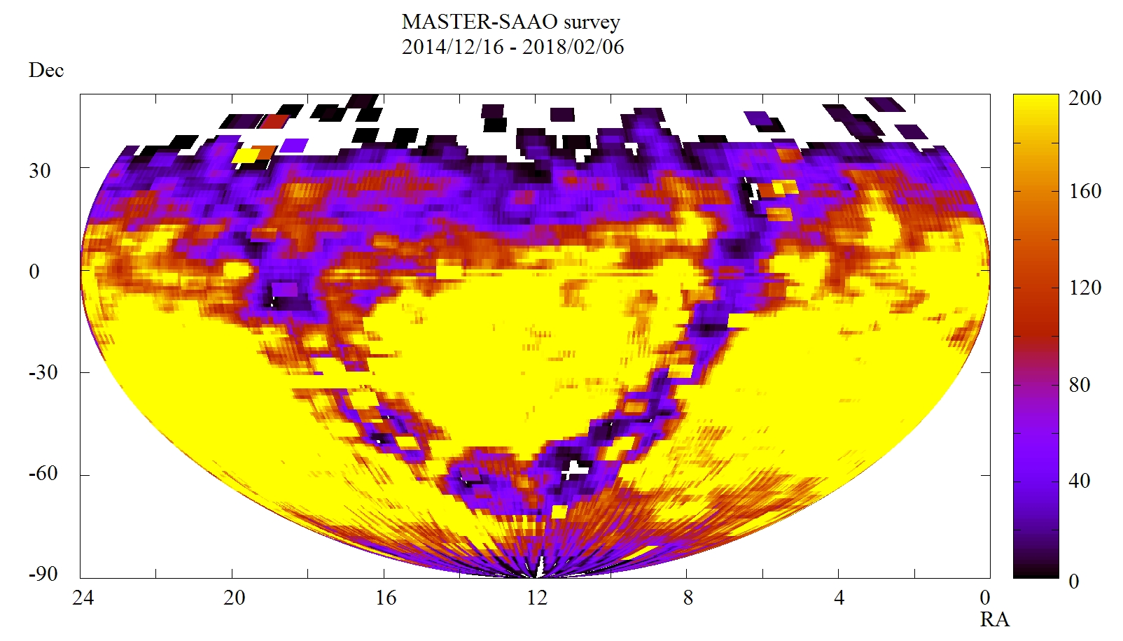
Figure 2: The MASTER–SAAO survey area, colour coded to indicate the number of visits per field for the period 2014 December to 2018 February.

The Mobile Astronomical System of Telescope-Robots (MASTER) (Lipunov et al., 2010; Kornilov et al., 2012) is a network of optical transient detection systems, the initial five situated in Russia, with three more recent nodes established elsewhere: MASTER-SAAO at the South African Astronomical Observatory (SAAO), MASTER-IAC in Spain at Instituto de Astrofísica de Canarias (IAC, Tenerife) and MASTER-OAFA at the Observatorio Astronomico Felix Aguilar of San Juan National University in Argentina (Lipunov et al., 2016).

The MASTER survey detects a range of transient types, including Galactic sources (CVs, flare stars, novae, deeply eclipsing binaries), AGN (blazars), supernovae and Solar System objects. All the MASTER nodes can also undertake follow-up on transient alerts from other facilities, for example detecting the optical emission from GRBs or optical counterpart searches of gravitational wave or neutrino events. Each telescope can observe with one of four filters ($\it{B,V,R}$ or $\it{I}$) or with polarizing filters. As well as the twin 0.4-m telescopes, each mount also has 2 Very Wide Field (VWF) cameras, covering $\sim$1000 deg², but with a shallow limit of unfiltered ${\sim}12\,$mag in a 1 s exposure, and $15\,$mag for a 10 min exposure.

The MASTER-SAAO node was installed and commissioned over a $\sim$3 week period, becoming operational in late December 2014. A clam shell dome allows rapid slewing over the entire sky, with declination limit of $-90{\,{}^{\circ}}$ to $+40{\,{}^{\circ}}$. There is no limit on the Galactic latitude, although the Galactic plane is a lower priority region for MASTER–SAAO, so the cadence is considerably less (by 10–20 times) than for higher Galactic latitudes. In Figure 2 we show the survey area of MASTER-SAAO, which also indicates the number of visits for each position in the survey region.

In Table 1 we compare some of the MASTER survey parameters with those of the Catalina Real-time Transient Survey (CRTS) (Drake et al., 2009), which until recently has been the only other transient detection system for which a study of CVs has been reported in some detail by Drake et al. (2014). We attempt to make a comparison between the entire MASTER and CRTS networks, as well as with the two systems specific to the southern hemisphere, namely the MASTER-SAAO node in South Africa and the Siding Spring Survey (SSS) of CRTS in Australia (which ceased operations in 2013). While we have attempted to present the best estimates of the survey parameters, there are some inevitable uncertainties due to lack of published information and the fact that some of the parameters are dependent upon season, Moon phase and observing conditions.

Figure 3: The on-sky instrument field-of-view in equatorial J2000 coordinates for the photometric data collected on J0614–27 from the SAAO. See Table 2 for details. The slight offset between images is due to manual telescope pointing.

2.2 The discovery of J0614–27

The MASTER-SAAO auto-detection system (Lipunov et al., 2010) discovered the transient source J0614–27 on 2015 February 19 (Shumkov et al., 2015) at 23h 17m U.T at the position:

$$\alpha_{2000} ={\ 06}^{\mathrm{h}}{14}^{\mathrm{m}}{51.70}^{\mathrm{s}}$$

$$\delta_{2000} ={-27}{\,{}^{\circ}}{25}^{\mathrm{{}^{\prime}}}{35.5}^{\mathrm{{}^{\prime\prime}}}$$

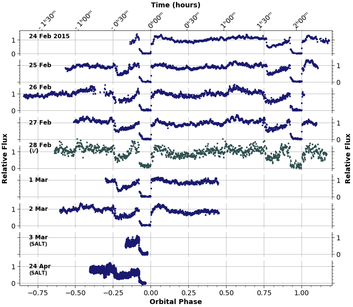
Figure 4: Light curves of J0614–27 obtained in period 24 Feb – 24 Apr 2015 using the SHOC high speed camera on the SAAO 1.9-m and 1.0-m telescopes (upper 7 light curves), as well as SALTICAM on SALT (lower 2 light curves). The eclipse and pre-eclipse dip, due to the obscuring accretion stream, are clearly seen. All light curves are unfiltered (or clear filtered for SALT), save that of 28 Feb, which is $V$-band filtered. Each light curve is displayed on the same scale in units of relative flux.

The unfiltered magnitude was ${\sim}18.3$ from the three consecutive images and the limiting magnitude of the reference image, taken on 2015 February 6.92896, was 19.4. There is one previous image of J0614–27 in the MASTER-SAAO database, taken on 2015 January 10.996, where it was just detected at the 18.8 magnitude limit of the exposure. Further interrogation of this region with Aladin has revealed a faint blue object, just above the limit, in the DSS UKSTU-blue survey image while there is also a weak GALEX source coincident with the J0614–27 position. This source is catalogued as GALEX J061451.7-272534.

Table 2: Photometry observation log for J0614–27.

Date	Time Start	Duration	Exposure	Filter	Telescope	Accretion	Figure
	(UTC)		Time (s)			State
2015-02-24	18:15:36	${3}^{\mathrm{h}}{26}^{\mathrm{m}}{20}^{\mathrm{s}}$	15	–	SAAO 1.9m	high	4
2015-02-25	18:19:05	${3}^{\mathrm{h}}{28}^{\mathrm{m}}{38}^{\mathrm{s}}$	10	–	SAAO 1.9m	high	4
2015-02-26	18:41:14	${3}^{\mathrm{h}}{51}^{\mathrm{m}}{59}^{\mathrm{s}}$	10	–	SAAO 1.9m	high	4
2015-02-27	18:14:32	${3}^{\mathrm{h}}{20}^{\mathrm{m}}{48}^{\mathrm{s}}$	10	–	SAAO 1.9m	high	4
2015-02-28	18:55:15	${3}^{\mathrm{h}}{45}^{\mathrm{m}}{06}^{\mathrm{s}}$	15	V	SAAO 1.9m	high	4
2015-02-28	18:40:16	${4}^{\mathrm{h}}{00}^{\mathrm{m}}{02}^{\mathrm{s}}$	45	R	SAAO 1.0m	high
2015-03-01	18:29:20	${1}^{\mathrm{h}}{33}^{\mathrm{m}}{23}^{\mathrm{s}}$	10	–	SAAO 1.9m	high	4
2015-03-02	19:16:22	${1}^{\mathrm{h}}{33}^{\mathrm{m}}{23}^{\mathrm{s}}$	10	–	SAAO 1.9m	high	4
2015-03-03	20:37:31	${0}^{\mathrm{h}}{18}^{\mathrm{m}}{58}^{\mathrm{s}}$	0.5	clear	SALT	high	4
2015-04-24	17:16:26	${0}^{\mathrm{h}}{45}^{\mathrm{m}}{41}^{\mathrm{s}}$	0.5	clear	SALT	high	4
2017-02-08	19:16:22	${2}^{\mathrm{h}}{30}^{\mathrm{m}}{01}^{\mathrm{s}}$	45	–	SAAO 1.0m	low	7
2017-02-09	18:45:48	${2}^{\mathrm{h}}{30}^{\mathrm{m}}{01}^{\mathrm{s}}$	45	–	SAAO 1.0m	low	7
2017-03-24	02:36:58	${0}^{\mathrm{h}}{24}^{\mathrm{m}}{40}^{\mathrm{s}}$	12	GG420	MDM 1.3m	low
2017-10-20	11:39:47	${0}^{\mathrm{h}}{18}^{\mathrm{m}}{26}^{\mathrm{s}}$	20	GG420	MDM 1.3m	low
		${29}^{\mathrm{h}}{17}^{\mathrm{m}}{25}^{\mathrm{s}}$

3 High speed optical photometry

3.1 Data acquisition and light curve extraction

J0614–27 was observed at the SAAO Sutherland station as part of a wider follow-up programme on new CV and transient discoveries resulting from the MASTER–SAAO survey (amongst others). Time resolved (10–45 s resolution) photometry of J0614–27 was obtained with both the SAAO 1.9-m and 1.0-m telescopes during a two week campaign in 2015 February, with less extensive observations following up in 2017 February (see Table 2 for a detailed observing log). Observations were undertaken with the Sutherland High-speed Optical Camera (SHOC) instruments, which utilise Andor iXon888 CCD cameras with 1024 $\times$ 1024 pixel CCDs (Coppejans et al., 2013). Light curves spanning 1.5–4.0 h were obtained on 7 different nights, mostly with a clear filter. The field of view was ${\sim}1.3^{\prime}\times 1.3^{\prime}$ for the 1.9-m observations and ${\sim}2.8^{\prime}\times 2.8^{\prime}$ for the 1.0-m (see Figure 3). In addition, short time series were obtained in 2017 March and October using the 1.3m McGraw-Hill telescope at MDM observatory, the former with a SiTE 1024 $\times$ 1024 CCD detector and the latter with an Andor Ikon camera similar to SHOC. The MDM observations served to confirm the cycle count.

In addition to the SAAO and MDM data, photometry was done at a higher time resolution of 0.5 s, using SALTICAM in ‘slot mode’ on SALT during the nights of 3 March and 24 April 2015. Reduction of the SAAO SHOC CCD data was performed using the pySHOC library; an open-source, object-oriented python library built off the standard SHOC reduction pipeline. Calibration of the raw CCD frames, included subtraction of median bias and dark frames, as well as flat-field correction with median frames constructed from exposures of the uniformly illuminated evening twilight sky. Aperture photometry was used to extract the light curves of all stars in the calibrated science images. pySHOC uses the photutils library (Bradley et al., 2016) as a backend for performing aperture photometry. The aperture positions were chosen by tracking the average centroid positions of the brightest stars in the frame, while the aperture sizes were chosen based on the dispersion (standard deviation / FWHM) of a Gaussian point source function (PSF) fitted simultaneously to all stars using a least-squares optimization. In this way, the aperture size adjusts to any changes in seeing that occur during the run to ensure optimal signal-to-noise extraction. Sky annuli for background subtraction were similarly scaled. Differential photometry was done on the background subtracted light curves by co-adding the signals of all non-variable stars in the field into a single time series which was used to compute the differential flux of J0614–27. Finally, points in the light curves with large uncertainty (due to inferior atmospheric conditions or too-bright background) were removed from the final product light curve shown in Figure 4.

Extraction of the SALTICAM light curves required a number of additional steps. In particular, the SALTICAM images are affected by vignetting from the slit mask, as well as by PSF degradation due to drift in the primary mirror alignment on SALT (active, closed-loop alignment of mirror segments was not operational at the time of the observation). Since our target star was positioned near the edge of the frame for at least one of the SALTICAM runs, we modelled the background vignetting pattern with a smooth, piecewise polynomial in order to remove its effect and produce a more accurate flux measurement. Additionally, the comparison star was (unintentionally) positioned on a region of the CCD containing a number of bad pixels which have a lower response than their neighbours. If uncompensated for, the small frame-to-frame dither during the observation leads to spurious variation that is purely instrumental in origin being introduced by these pixels. Since no calibration flats are available for SALTICAM, an artificial flat field image was constructed from the last ${\sim}120$ frames of the observation (off-target sky images) by comparing the value of each pixel in the array with the median value of its 8 nearest neighbour pixels, and averaging this ratio across all available frames. The flat field image produced in this way effectively normalised the pixel response and improved the quality of the photometry. To compensate for the PSF degradation, an optimization step was performed at each image in order to select the highest SNR aperture for the stars. This step involves maximizing the totalled SNR for elliptical apertures across 3 parameters (height, width and rotation) given the data. The aperture fluxes obtained from the optimal apertures were then processed as above to obtain the final SALTICAM light curves.

4 Light curve characteristics

In Figure 4 we show all the differential light curves we obtained during our 2015 campaign on J0614–27. The most prominent feature in the light curve is a deep eclipse during which the source brightness decreases to the level of the background sky. In addition, there is a shallower eclipse-like feature, or dip, preceding the primary eclipse and lasting ${\sim}4$ min. This pre-eclipse dip comprises an initial sharp drop in brightness to ${\sim}50$% of the out-of-eclipse level, followed by a slower recovery back to nominal brightness. The rapid ingress of the primary eclipse then occurs, followed by an approximately linear decline of intensity over ${\sim}3$ min into a total eclipse. A rapid egress occurs some ${\sim}6.5$ min later. The features immediately following the primary egress remain highly variable from night to night. Sometimes a stepped feature can be seen $20--30\,$s after the start of primary egress. This is most clearly visible in the light curves on 2015 February 24 (both eclipses: E0, E1) and February 25 (second eclipse: E13) (see Figures 4 and 6). In general, the post-egress light curve tends to gradually increase in brightness towards a level comparable to that of pre-eclipse. The exceptions being that of 2015 February 25 (E12) and March 1 (E70) where the gradual brightening phase is much less pronounced, and the egress step brings the source almost directly back to the pre-eclipse level.

We identify the components of the light curve as follows: The pre-eclipse dip is most likely due to an accretion stream obscuring a bright accretion spot(s) on the white dwarf, while the deep eclipse evidently arises from the secondary star passing in front of this bright spot. The residual brightness remaining after the primary eclipse can be attributed to the illuminated portion of the accretion stream which still remains visible beyond the limb of the secondary star. Similarly, the post-egress recovery, is most likely due to the egress of the illuminated accretion stream. Superficially, the light curve of J0614–27 appears very similar to that of HU Aqr presented in (Harrop-Allin et al., 1999), the most distinct difference being the prominence of the pre-eclipse dip in J0614–27.

There is some variability in the phase of the pre-eclipse dip: A nightly shift is typically around 0.03 in phase, corresponding to an angular variation of ${\sim}10{\,{}^{\circ}}$ of the obscuring portion of the stream with respect to the bright spot. Comparing the light curves in Figure 7: The 2017 data were acquired while the source was in a lower accretion state and therefore appeared significantly fainter for most of the orbit. There are a number of interesting differences between the low- and high-state light curves, most notably the phasing of the pre-eclipse dip. The differences between the low- and high-state light curves are discussed in section 8 below.

Stochastic flickering, with an amplitude as much as ${\sim}20$% of the peak intensity, is seen in the light curves, with a characteristic timescale of ${\sim}200\,$s. This is particularly evident at $0.5\lesssim\phi\lesssim 0.8$ (e.g. on February 26 & 27), prior to the dip. In contrast to the high-frequency flickering often observed in polars with timescales of seconds (e.g. VV Pup), the flickering in J0614–27 occurs on a time-scale of minutes. Our data lack the time resolution to search for signatures of other rapid variability such as Quasi-periodic oscillations (QPOs) that occur in some mCVs during their bright phases (e.g. V834 Cen (Mouchet et al., 2017)).

4.1 Period analysis

The most precise phase fiducial in the light curve (detailed in the next section) appears to be the sharp egress from eclipse. Since the SALTICAM light curves do not cover the eclipse egress, they were excluded for the ephemeris calculation. The remaining observations define a unique ephemeris,

$$\mathrm{BJD\,(egress)}=2457078.2747(1)+0.08660831(2)\,E$$ (1)

where $E$ is the integer cycle count. Table 3 gives timings of the sharp egress; the predicted times are computed using the ephemeris above. The cadence of our data is insufficient to resolve the egress, so we are not able to estimate meaningful uncertainties for the egress times from the data alone, save to say that we are confident we can interpolate the half-egress point to an accuracy significantly better than our sampling interval. The uncertainty in the measured egress timings is estimated from the residuals of the linear ephemeris. We have 12 egress timings, spanning two years, with an rms scatter of $5.4$ sec, which is half of our typical cadence.

Table 3: Ephemeris of eclipse egress times for J0614–27. Observed/predicted times given are full Julian days minus 2450000. The second-to-last columns gives the O$-$C error in units of seconds, while the last column gives that in units of $\sigma_{E}$ - the estimated standard deviation uncertainty of the ephemeris.

$E$	Observed	Predicted	O$-$C
			s	$\sigma_{E}$
0	7078.2748	7078.2747	4	0.5
1	7078.3614	7078.3613	5	0.6
12	7079.3140	7079.3140	$-$1	0.1
13	7079.4005	7079.4006	$-$12	1.4
35	7081.3060	7081.3060	$-$3	0.4
36	7081.3927	7081.3926	3	0.4
58	7083.2981	7083.2980	3	0.4
8256	7793.3129	7793.3128	9	1.0
8257	7793.3994	7793.3994	0	0.0
8268	7794.3521	7794.3521	$-$1	0.1
8756	7836.6173	7836.6171	1	0.1
11185	8046.9884	8046.9885	$-$7	0.8

Since the eclipse egress provides a well constrained marker for timing analysis, we do not need to rely on a frequency analysis to determine the orbital period. Nonetheless, we performed a frequency-spectral estimation using the Lomb-Scargle technique (Lomb, 1976; Scargle, 1982; VanderPlas & Ivezić, 2015) in order to search for hidden periodicities, and possible quasi-periodic variability at higher frequencies. Figure 5 shows the periodogram computed using the gatspy python package (Vanderplas, 2015). We see no indication of significant periodic variability not associated with the orbital variation and its harmonics.

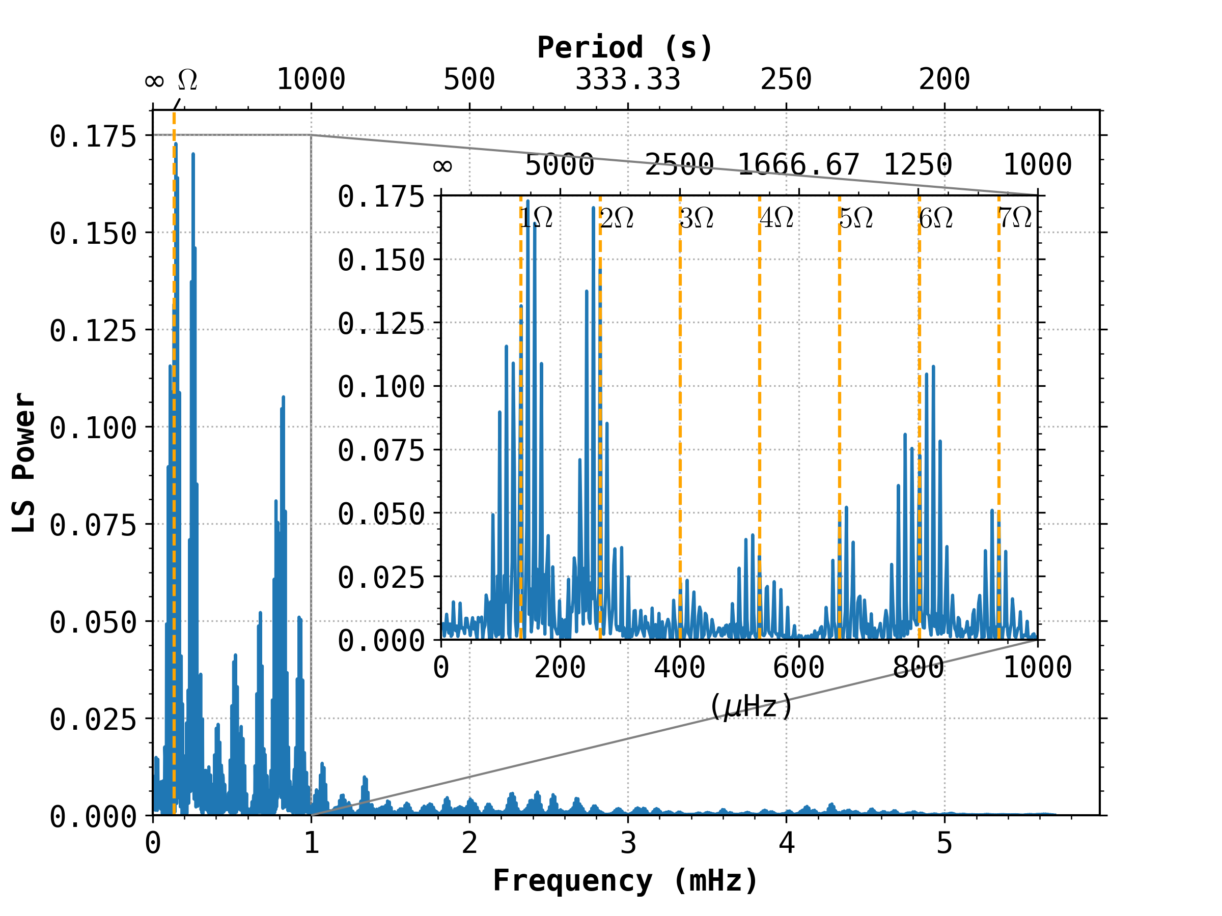
Figure 5: The Lomb-Scargle periodogram of the combined light curve data of J0614–27. The most prominent peak in the periodogram is due to the orbital variation and its harmonics (the orbital period is indicated by the dashed orange line). The inter-day alias structure due to the observing cadence is also clearly seen in the inset panel as the separation between adjacent peaks.

4.2 Measuring the eclipse profiles

Figure 6 shows the succession of the eclipse light curves for the 2015 data for a phase range of $0.7<\phi<1.1$. The steep initial decline of the first dip, followed by a steady recovery in intensity, followed by the eclipse are clearly seen. We present the measured phase duration of various parts of the eclipse (labelled in the bottom panel of Figure 6) in Table 4. The values presented here were, in each case, obtained by measuring the durations of each component in the individual light curves (using only the 2015 data). The values in Table 4 are the means of the individual measurements, while the uncertainties are their $1\sigma$ standard deviations.
The width of the primary eclipse was measured as the full width at half depth (FWHD). The out-of-eclipse brightness used as a reference point to measure the depth of the eclipse is taken as the averaged brightness in phase bins of width 0.025 immediately preceding/following the primary eclipse. It was found that the resulting FWHD measurement is relatively insensitive to the choice of bin size for measuring the out-of-eclipse brightness.
To measure the duration of the ingress / egress, we refer to the point-to-point difference estimate for the light curve derivative. Due to the presence of flickering noise from the accretion process, it is not possible to distinguish the ingress/egress of the WD as distinct from that of the accretion column / bright spot given our data. We therefore refer to the combined observation of both these features as the primary ingress. The start of the primary ingress/egress is taken as the point preceding that at which there is a significant change in the derivative estimate. Here it proved sufficient to use the Generalized Extreme Studentized Deviate (GESD) Test (Rosner, 1983) to identify the outlying points marking the start of the ingress and egress. The end of the ingress/egress is taken as the point preceding that at which the point-to-point derivative again returns to nominal (inlying) values. Using this method to measure the ingress and egress duration from the data implies that the uncertainty on our measurements is at least as large as the time resolution (exposure time) of each light curve. We note furthermore that the size, shape, and position of the accretion column, as well as any brightness variability within it (which we know occurs on timescales shorter than the orbital period) will also affect these measurements. The time (phase) resolution of the light curves from the smaller telescopes (SAAO 1.0-m and 1.9-m) is insufficient to resolve the primary ingress/egress. The two SALT light curves (2015 March 3 and April 24), however, do resolve the primary ingress, but where terminated mid-eclipse, and therefore do not resolve the egress. The egress duration presented in Table 4 should therefore be interpreted as an upper limit only.
The ingress of the lower portion of the stream starts immediately after the primary ingress and ends at the start of totality. The start of totality is taken as the time corresponding to the first data point which falls below $1\sigma$ of the in-totality noise level. To measure the duration of the pre-eclipse dip, and the ingress duration of the upper portion of the stream, the point-to-point numerical derivative proved inefficient, due to the high variability in this part of the light curve. Instead, we use a smooth estimate of the derivative obtained by a total variation regularization procedure. A detailed implementation of this procedure is presented in Stickel (2010). This method is similar to the edge-preserving derivative estimator used by Spark & O’Donoghue (2015) to investigate the variability of the boundary layer in the eclipsing non-magnetic CV, OY Car. We find that the start and end of the dip ingress can reliably be detected by selecting the phase regions in which the optimally smooth derivative remains negative and has magnitude greater than the local outlier (GESD) threshold as described above.
Finally, we note that, in terms of measuring the eclipse parameters, the influence of noise from short timescale variability may be mitigated by incorporating effect of flickering in the modelling procedure, as done in e.g. McAllister et al. (2017), although doing so is beyond the scope of this work.

Table 4: Measured duration of various parts of the eclipse light curve of J0614–27. The segments listed here are illustrated graphically in the bottom panel of Figure 6.

	$\Delta\phi$		$\Delta\phi$ (${\,{}^{\circ}}$)		$\Delta t$ (s)
Upper stream ingress ($\Delta\phi_{S1}$)	0.029 $\pm$	0.007	10.0 $\pm$	2.5	216 $\pm$	50
Primary ingress ($\Delta\phi_{\mathrm{I}}$)	0.0007 $\pm$	0.0001	0.24 $\pm$	0.05	5 $\pm$	1
Lower stream ingress ($\Delta\phi_{S2}$)	0.0233 $\pm$	0.0012	8.4 $\pm$	0.4	174 $\pm$	9
Totality ($\Delta\phi_{T}$)	0.0548 $\pm$	0.0014	19.7 $\pm$	0.5	410 $\pm$	10
Primary Egress ($\Delta\phi_{E}$)	0.0025 $\pm$	0.0008	0.9 $\pm$	0.3	$19\ ^{*}$
Eclipse FWHD ($\Delta\phi_{F}$)	0.0780 $\pm$	0.0004	28.08 $\pm$	0.14	583.8 $\pm$	2.7
* upper limits

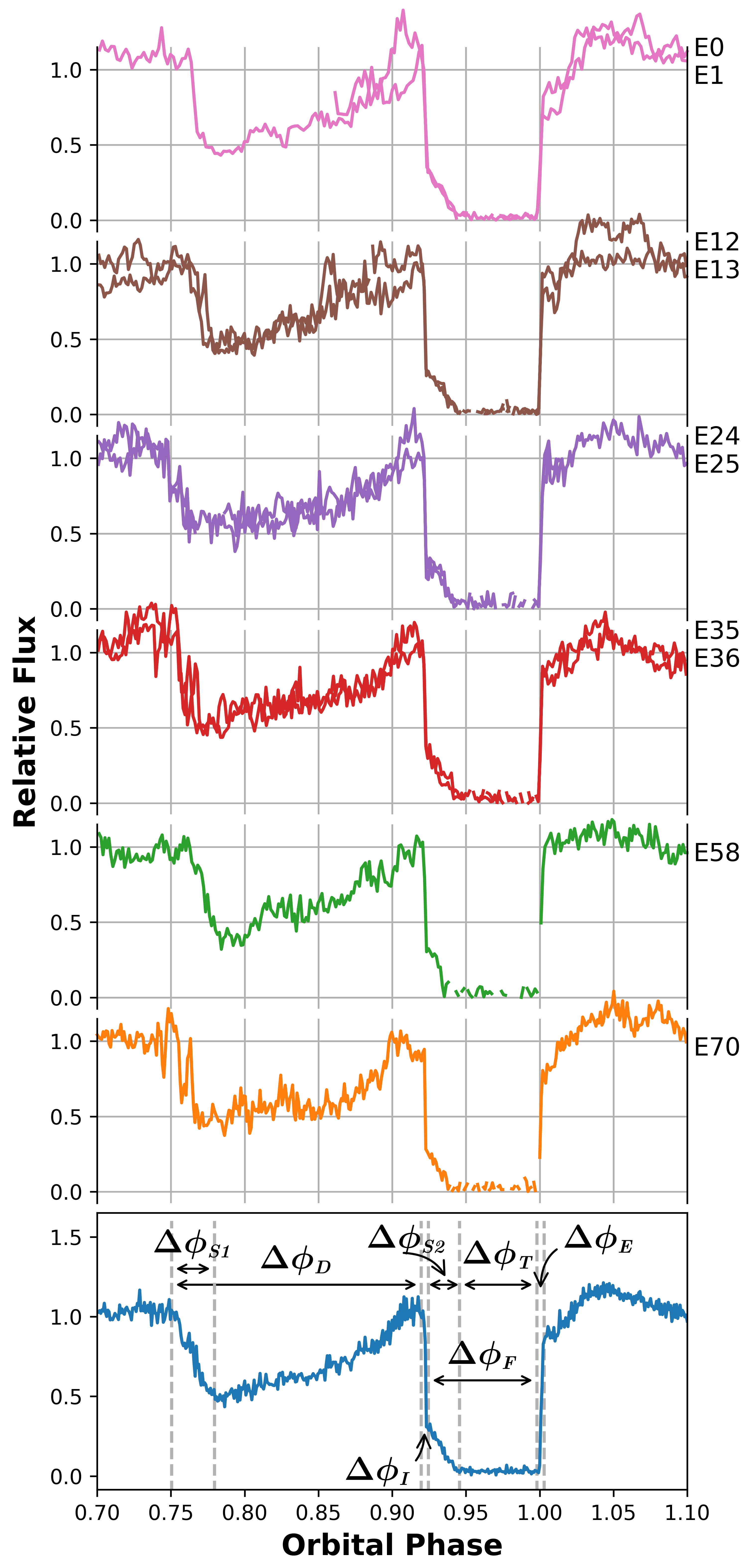
Figure 6: The 10 eclipses of J0614–27 observed over 6 nights of observing during our 2015 campaign. The cycle counts from the ephemeris in Equation 1 are indicated next to the light curves on the right of the figure. The bottom panel shows the average light curve with the various phases of the eclipse marked and labelled (see also Table 4).

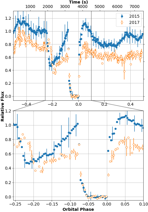
Figure 7: Average phase folded light curves of J0614–27 comparing the high-state (filled blue circles) and low-state (open orange circles) runs. Uncertainties on the data points are indicated by vertical bars. The source was significantly fainter in 2017. The most prominent change in the eclipse profile between the two runs is the phase of the pre-eclipse dip, most likely due to changes in the location and/or radius of the threading region. The upper panel compares the light curve across the full orbital cycle, while the bottom panel shows a zoom-in of the eclipse. The differences between the low-state and high-state light curves are discussed in the text of section 8.

5 Spectroscopy

J0614–27 was observed with the SALT (Buckley et al., 2006) during our photometry campaign using the RSS (Burgh et al., 2003; Buckley et al., 2008) on 2015 February 28 at 21:10 U.T., with the mid-time of the observation at HJD = 2457082.3881. The PG900 grating and slit 1.25 arcsec width were used for observations. The spectrum covers spectral region 4060$-$7120 Å, with a final reciprocal dispersion of $0.97$ Å$\cdot$pixel^-1. The spectral resolution full width at half-maximum (FWHM) is $4.40\pm$0.15 Å. The total exposure time was 800 s. An Ar arc lamp spectrum was taken immediately after science frame. Spectrophotometric standard stars were observed during twilight time for relative flux calibration. Absolute flux calibration is not feasible with SALT since the size of the unfilled entrance pupil changes during the observations as the telescope tracks. Primary reductions of the data was done in the standard way with the SALT science pipeline (Crawford et al., 2010). We reduced the long-slit spectroscopic data using procedures described by Kniazev et al. (2008). The resulting normalized spectra are presented in Figure 8. Equivalent widths (EWs), FWHMs and heliocentric radial velocities (RVs) of some lines in the spectra were measured applying the midas programs (see Kniazev et al. (2004) for details) and are given in Table 5. The spectrum shows all of the Balmer lines in emission, a strong He ii 4686 Å line, at a peak flux greater than H$\beta$, and weaker He i lines, all superimposed on a continuum rising to the blue. The lines appear asymmetric and structured, with wings extending to shorter wavelengths. We note that the average radial velocity of the lines is -230 km s^-1, consistent with the observation being at orbital phase $\phi=0.49$, when the white dwarf is closest to us and the accretion stream from the secondary is expected to have a net blue-shifted velocity as it is approaching us.

Table 5: Emission line parameters for J0614–27.

$\lambda_{0}$ (Å)	Line	E.W. (Å)	FWHM (Å)	R.V. (km s-1)	Relative Flux
4101	H$\delta$ + He ii	$18.67\pm 0.66$	$14.52\pm 0.55$	-$242\pm 17$	$26.3\pm 0.9$
4340	H$\gamma$ + He ii	$28.68\pm 0.83$	$21.67\pm 0.66$	-$209\pm 19$	$34.6\pm 1.0$
4471	He i	$6.06\pm 0.46$	$20.67\pm 1.44$	-$200\pm 40$	$7.1\pm 0.5$
4686	He ii	$23.10\pm 0.71$	$15.81\pm 0.50$	-$234\pm 13$	$27.0\pm 0.8$
4861	H$\beta$ + He ii	$28.83\pm 0.84$	$22.84\pm 0.68$	-$239\pm 18$	$33.6\pm 1.0$
4922	He i	$2.77\pm 0.36$	$10.21\pm 1.12$	-$214\pm 29$	$3.2\pm 0.4$
5016	He i	$1.73\pm 0.27$	$9.17\pm 0.96$	-$225\pm 24$	$2.0\pm 0.3$
5412	He ii	$3.92\pm 0.45$	$13.95\pm 1.37$	-$189\pm 32$	$4.2\pm 0.5$
5876	He i	$6.84\pm 0.53$	$18.24\pm 1.06$	-$263\pm 23$	$6.2\pm 0.5$
6563	H$\alpha$ + He ii	$26.56\pm 1.03$	$24.00\pm 0.85$	-$201\pm 17$	$20.4\pm 0.8$
6678	He i	$5.32\pm 0.53$	$19.24\pm 1.44$	-$245\pm 27$	$3.8\pm 0.4$

The spectrum of J0614–27 is typical of an mCV, particularly with the strong He ii 4686 Å line. Therefore, considering the spectral features together with the features in the light curve – the rapid and deep eclipses as well as the pre-eclipse “dip” and the absence of other periodicities – the evidence points to J0614–27 being new eclipsing polar.

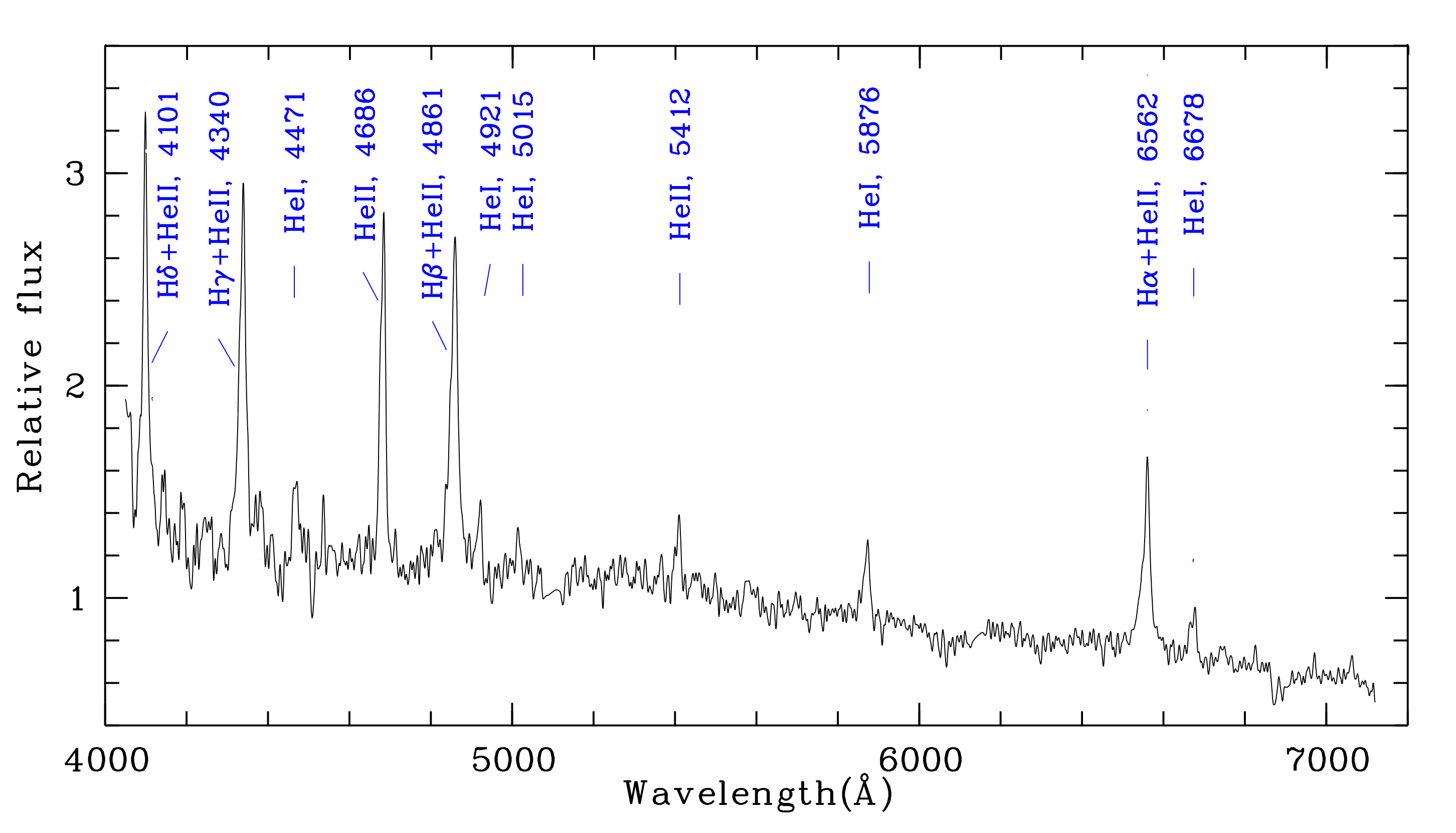
Figure 8: A SALT RSS spectrum of the eclipsing polar, J0614–27.

6 Modelling the eclipse and pre-eclipse dip

The light curve of J0614–27 is characterised by a typical polar-like eclipse profile, where the eclipse is dominated by the rapid ingress and egress of the accreting pole on the WD surface. This is preceded by a deep and very wide absorption feature or dip. This feature is much more prominent than usually seen in polars, as it is both much deeper and more extended in orbital phase. The eclipse of the accretion stream is characterised by the slow and linear transitions after the pole ingress and egress. The depth and substantial phase extent of the absorption dip implies somewhat unusual accretion geometry. In order to investigate the physical origin of the eclipse light curve, we have employed the eclipse mapping approach of Hakala et al. (2002), which aims to provide three-dimensional mapping of the accretion stream and has previously been used to model the light curves of a number of other polars (Bridge et al., 2004).

Hakala et al. (2002) constructed a gridless 3D model for the accretion stream, where the stream was modelled by a swarm of “fireflies” i.e. emission points of equal brightness, that were free to move within the Roche lobe of the primary. As such the model has far too much freedom when compared to the information content of the data, and some regularisation is required. The model was regularised by preferentially selecting firefly distributions that follow a smooth trajectory from the L1 point to the WD surface. This was achieved by first solving the smoothest possible line through any swarm of fireflies using a self-organizing map (SOM) algorithm (Kohonen, 1990). The deviations of fireflies from this trajectory were then minimised, together with the $\chi^{2}$ for the fit (see the original paper of Hakala et al. (2002) for more details).

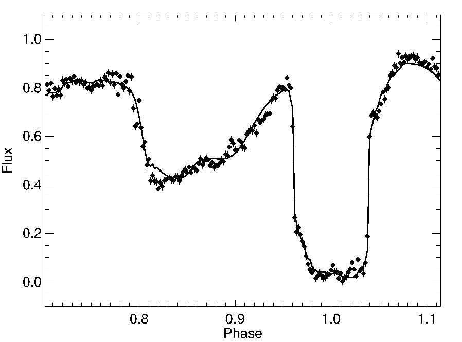
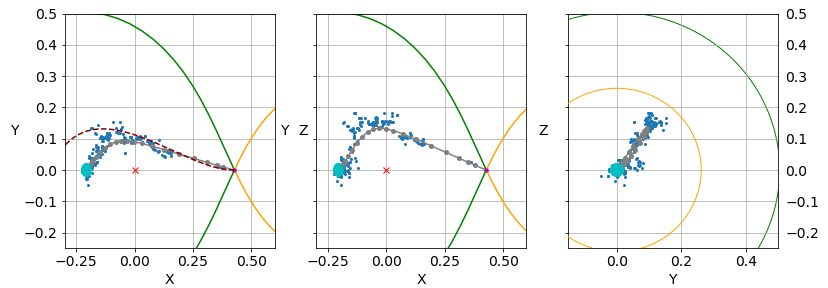
Figure 9: Upper panel: The accretion stream model fit to the average 2015 light curve of J0614–27. Lower panel: A view into the accretion geometry. Each panel provides a two-dimensional projected view of the system in units of the binary separation $a$. Shown in grey is the trajectory of the accretion stream derived from the “firefly” model. The best fitting model shows the stream trajectory that moves above the orbital plane by up to $10R_{\mathrm{WD}}$. The scattered blue dots around the final stream solution are the positions of the individual fireflies used to derive the fit. The position and radius of the WD are indicated by the cyan dot. The centre of mass of the system (red cross), as well as the Roche lobes of both stars are also partially shown. The leftmost panel (view from above the orbital plane) also shows a typical single particle ballistic trajectory for a hydrogen particle entering the system at the L1 point with thermal velocity typical of a late M–type dwarf at 3000 K. The system parameters used to construct these plots are derived in section 7.

Hakala et al. (2002) did not model any dips and therefore the original model did not include any absorption. Clearly absorption is required here, so the model was updated. As the distribution of fireflies mimics the mass distribution of the stream, we implemented the first order model for the absorption by simply associating a 3D Gaussian optical thickness profile for each firefly and integrated the optical depth from the WD along the line of sight. The self-absorption of the stream emission was not considered. We experimented with various Gaussian widths, but the results were not strongly dependent on the exact choice thereof.

The orbital inclination, $i$, is not known, but since the system is eclipsing, we may constrain it to be greater than $75{\,{}^{\circ}}$. To further constrain the inclination, we used our code to compute the eclipse widths for a range of $(q,i)$ pairs. For each value of inclination we examined a grid of q values to reproduce the observed eclipse width for the pole. The results are tabulated in Table 6. The $(q,i)$ values remain fixed during each eclipse profile modelling run.

Table 6: Possible combinations of inclination ($i$) and mass ratio ($q$) pairs based on the observed eclipse width.

$i$	$76{\,{}^{\circ}}$	$78{\,{}^{\circ}}$	$80{\,{}^{\circ}}$	$82{\,{}^{\circ}}$	$84{\,{}^{\circ}}$	$86{\,{}^{\circ}}$	$88{\,{}^{\circ}}$
$q$	0.713	0.543	0.420	0.332	0.272	0.233	0.211

We find that best fits are obtained with intermediate inclination values around 80 degrees, even if our modelling cannot be used to constrain the inclination properly. This is because the $\chi^{2}$ values of different fits cannot be formally compared due to the regularisation of the model. The resulting light curve, together with the best fitting model is shown in Figure 9. The underlying 3D model of the accretion stream (distribution of fireflies) with its associated regularisation reference (20 nodes calculated using SOM) is shown in Figure 9. Our modelling suggests that the wide dip preceding the eclipse is likely to be produced by a relatively wide accretion stream/curtain in the magnetically controlled part of the stream near the WD. The stream appears to be following a trajectory, where it is taken well above the orbital plane (up to ${\sim}10R_{WD}$) soon after leaving the L1 point. The stream impacts the WD at a ${\sim}45{\,{}^{\circ}}$ angle with respect to the orbital axis, and a ${\sim}40{\,{}^{\circ}}$ azimuthal angle, with respect to the line of centres. The horizontal and vertical extents of the stream are very similar. Most of the stream emission arises within $0.3\,a$ of the WD, where $a$ is the binary orbital separation.

The results of the modelling are presented in Figure 9 where we show in the upper panel, our model fit to the eclipse and the stream absorption feature. The model stream trajectory, as well as the firefly distribution from which it was derived, is show in the bottom panel of Figure 9.

7 Binary system parameters

Using the semi-empirical evolutionary models of (Knigge et al., 2011, supplementary Table 6), we estimate the donor mass and radius from the orbital period as $M_{2}=0.163\,M_{\odot}$ and $R_{2}=0.202\,R_{\odot}$. Since we are able to measure the orbital period of J0614–27 very accurately (see subsection 4.1), the uncertainties in $M_{2}$ and $R_{2}$ can be considered to be purely due to the evolutionary model (the propagated uncertainty due to the period measurement is less than 0.05%). We note that the Knigge $M_{2}-R_{2}$ relation assumes a non-magnetic primary with a mass of $0.75\,M_{\odot}$. Any effects on the evolution of the system that are produced by magnetic activity (and/or rotation of the secondary) are therefore unaccounted for here. Since the model uncertainties are not made available in Knigge et al. (2011), it is difficult to assign uncertainties on the parameters $M_{2}$ and $R_{2}$. Based on the scatter of data points in the $M_{2}-R_{2}$ relation (Figure 4 in Knigge et al. (2011)), we expect a ${\sim}15\%$ uncertainty in these parameters.

Having measured the phase width ($\Delta\phi$) of the primary eclipse, we may place constraints on the inclination, $i$, and mass ratio, $q$, that are independent of the firefly model using the method of Chanan et al. (1976) (see also: Zdziarski et al. (2016)). For a given eclipse width, there is a degeneracy between the size of the secondary (which varies with q) and the inclination, since a larger secondary can eclipse the WD for the same duration of time as a smaller would at a higher inclination. Figure 10 illustrates the constraints graphically. The measured eclipse width and its $1\sigma$ uncertainty is shown spanning a narrow range of possibilities on the y-axis. Also shown are the level contours of the $q(i,\Delta\phi_{\nicefrac{{1}}{{2}}})$ relation corresponding to the values in Table 6. We can see from this figure that the $3\sigma$ constraints provided by the Roche geometry are consistent with those provided by the firefly model for $i>82{\,{}^{\circ}}$. The minimum allowed mass ratio (smallest secondary) corresponding to an inclination of $i=90{\,{}^{\circ}}$ is $q_{min}=0.192$ (the lowest contour in Figure 10).

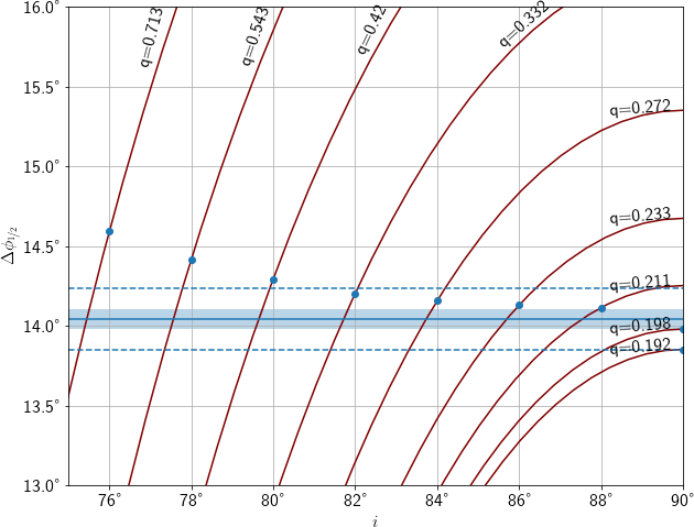
Figure 10: Constraints on the inclination of the system based on the eclipse phase width $\Delta\phi_{\nicefrac{{1}}{{2}}}$. Nine level contours of the $q(i,\Delta\phi_{\nicefrac{{1}}{{2}}})$ relation are shown as red curves crossing the axes diagonally. For each contour, a circular marker indicates the inclination value estimated from the firefly model. The measured eclipse half width (solid horizontal blue line), as well as its 1$\sigma$ (shaded horizontal region) and 3$\sigma$ uncertainties (dashed horizontal blue lines) are also shown.

With an inclination of $i>82{\,{}^{\circ}}$, we obtain a range of possible mass ratio values ${0.19\lesssim q\lesssim 0.33}$. With the secondary mass estimated from the evolutionary state, the corresponding range of possible values for the WD mass is ${0.5\,M_{\odot}\lesssim M_{1}\lesssim 0.86\,M_{\odot}}$. We note that this range is consistent with the distribution of WD masses in polars (see Zorotovic et al. (2011); Ferrario et al. (2015a)).

Using the Nauenberg (1972) WD mass-radius relation, we obtain the radius of the WD: ${R_{1}=0.014\pm 0.002\,R_{\odot}}$. The binary separation is calculated as ${a=3.25\pm 0.02\times 10^{-3}\,}$AU from Kepler’s third law. LABEL:tbl:params lists the derived system parameters and their uncertainties.

Table 7: Binary system parameters for J0614–27.

$P_{orb}$	$2.0786\pm 0.0009$ h	$7482.9\pm 3.5$ s
$M_{1}$	$0.5\,M_{\odot}\lesssim M_{1}\lesssim 0.86\,M_{\odot}$
$M_{2}$	$0.16\pm 0.03\ \,M_{\odot}$	$3.6\pm 0.6\times 10^{29}$ kg
$R_{1}$	$0.012\pm 0.002\ \,M_{\odot}$	$1.05\pm 0.07\times 10^{7}$ m	0.021 $a$
$R_{2}$	$0.20\pm 0.03\ \,R_{\odot}$	$1.4\pm 0.2\times 10^{8}$ m	0.286 $a$
$a$	$3.25\pm 0.02\ \times 10^{-3}$ AU	$4.86\pm 0.02\times 10^{8}$ m	1 $a$
$i$	$>82{\,{}^{\circ}}$

8 Discussion

Polars have been known for some time to show absorption dips in their X-ray light curves. Absorption dips were first noticed in soft X-ray light of EF Eri (Patterson et al., 1981), and have subsequently been observed in the light curves of a number of polars, most notably in V834 Cen, QQ Vul, AN UMa (King & Williams, 1985), QS Tel (Rosen et al., 1996), MN Hya (Buckley et al., 1998), CE Gru (Ramsay & Cropper, 2002), EV Uma, GG Leo (Ramsay et al., 2004) and AI Tri (Traulsen et al., 2010). Recently, (Wang et al., 2017) also detected absorption dips in the soft and medium X-ray light curve of the long period, low accretion rate polar J215544.4+380116. A number of IPs also display features in their soft X-ray and extreme-UV light curves characteristic of stream fed accretion near the WD: V709 Cas (de Martino et al., 2001; de Martino et al., 2004) and EX Hya (Belle et al., 2002).

Models that successfully explain the features of X-ray light curves were initially developed in King & Williams (1985) and Watson et al. (1989) and have subsequently been adapted to explain many features of the EUV light curves as well (Sirk & Howell, 1998). The most consistent idea is that the absorption dips are caused by (partial) occultations of the hot spot and post-shock region by magnetically threaded material at the magnetospheric boundary, or by material in the ballistic portion of the stream. The presence of P Cygni profiles at phases preceding the eclipse during the high state in HU Aqr (Schwope et al., 1997) and FL Cet (Schmidt et al., 2005) (amongst others) further support this interpretation.

Absorption dips in the visible light of Polars, seems to be somewhat less common. Besides the example of HU Aqr, already mentioned in section 4, another eclipsing polar, UZ For, has a pronounced stream absorption dip in the $R$-band light curve and, to a lesser extent, also in the $V$-band Bailey & Cropper (1991). The asynchronous polar V1432 Aql has an absorption feature that appears and disappears periodically, depending on the phase of the spin-orbit cycle. (Patterson et al., 1995). In general, the shape of the absorption features are strongly wavelength dependent, as can be seen from simultaneous multi-band photometry in Harrop-Allin et al. (1999). Other recent examples include LSQ1725-64 Fuchs et al. (2016), a deeply eclipsing polar with a symmetric stream absorption feature appearing during its bright state, as well as CSS081231:071126+440405 Schwope et al. (2015), another short-period polar with peculiar accretion geometry.

The flow structure in the inner regions of the binary can be quite complex. The interaction of the accretion stream with the magnetic field can manifest a wide variety of behaviours which depend sensitively on the mass transfer rate, magnetic field structure (strength and direction of the magnetic axis), the orbital period of the system, as well as the nature of the secondary star. Accretion flows which switch between the one- and two-pole regime has been observed in both QS Tel (Rosen et al., 1996) and MT Dra (Schwarz et al., 2002). Subsequent studies involving magneto-hydrodynamical simulations, have shown that accretion onto quadrupole Zhilkin et al. (2012, 2016) and octupole Long et al. (2012) field topologies are able to produce flows with multiple polar impact zones, or even azimuthally extended hot spots near the WD equator. There is also strong evidence from Zeeman-tomography that the WDs in (at least two) Polars are able to generate complex multi-polar field structures (Beuermann et al., 2007).

The way in which the material in the stream interacts with the magnetosphere of the accretor can therefore tell us something about the magnetic field of the primary star, as well as the mass transfer rate and properties of the plasma in the accretion stream. Ramsay & Cropper (2003), for example, use the stream absorption dip in the polar RX J1007.5$-$2017 to constrain the radius and total column density of the stream. In eclipsing systems in particular, much information is to be gained from the way in which luminous material is systematically mapped out by the occulting limb of the secondary. Observations of the low state light curves are particularly useful for modelling purposes since discerning the various luminous components in the binary becomes easier as the brightness of the stream and hot spot are diminished relative to the photospheric brightnesses of the stars. The diminished presence of the post shock accretion column can be seen in the low state light curve of J0614–27 in Figure 7 by the decrease in brightness across most of the orbit, as well as in the shallower eclipse profile.

Comparing the high-state (2015) and low-state (2017) light curves in Figure 7, we notice a number of additional differences: i) The absorption dip in the low state is narrower by ${\sim}10{\,{}^{\circ}}$ in phase as compared to the bright state. The position of the obscuring part of the stream has therefore shifted or narrowed by $10{\,{}^{\circ}}$ w.r.t. the line of sight to the bright spot. This could be explained by a change in the location (radius and/or azimuthal angle) of the threading region, or by a change in the location of the bright spot, or possibly a combination of both. Under a higher mass transfer regime, we expect the stream to penetrate deeper into the magnetosphere of the WD, and material to be threaded along a wider arc. This would lead to a larger accretion footprint extending to lower magnetic latitudes, which would show up as a phases shift in the position of the dip. We estimate that, at the location of the threading region indicated by the “firefly” model, a distance of $10\,R_{WD}$ from the WD, a change of $10{\,{}^{\circ}}$ in azimuth corresponds to a projected distance on the WD surface of ${\sim}0.4\,R_{WD}$. The accretion column would therefore have had to move a significant distance on the WD surface to reproduce the observed phase shift given an unmoving threading region. The possibility remains that observed shift is due to a slight asynchronism between the WD spin and the orbital period. In the near-synchronous eclipsing polar, V1432 Aql (Littlefield et al., 2015), discrepancies in the eclipse timings have been attributed to changes in the location of the threading region along the ballistic portion of the stream, and it is feasible that the same mechanism may be at work in J0614–27. The absence of any signature of periodic flux modulation due to the WD spin in Figure 5, along with the size of the nightly dip-phase shifts during 2015, however, suggest that the changes in the location of the threading region are due to mass transfer variability, rather than secular changes due to spin-orbit asynchronism.

ii) The shape of the absorption dip remains roughly unchanged between the high- and low-states and is highly asymmetric. If we assume that the luminosity of the bright spot/post-shock region remain constant across the phase range of the absorption dip, the asymmetry of this feature indicates that the leading edge of the threading region contains denser material than the trailing edge. This may be an indication of an inhomogeneous, or “blobby” accretion flow suggested by Kuijpers & Pringle (1982); Wynn & King (1995), since denser portions of the flow, being somewhat diamagnetic, would follow a ballistic trajectory deeper into the WD magnetosphere and eventually become threaded at a higher magnetic field value.

iii) The portion of the stream visible after the bright spot has been eclipsed eclipse remains equally bright in both states indicating that there is a significant amount mass transfer even during the low state.

iv) The average high-state light curve contains a centered at phase ${\sim}0.4$. The phase of this feature is such that it is located diametrically opposite the location of the primary ingress i.e. opposite the bright spot. This feature may be due to an azimuthally extended accretion hot spot visible on the far side of the WD, or potentially to the presence of a second accretion pole.

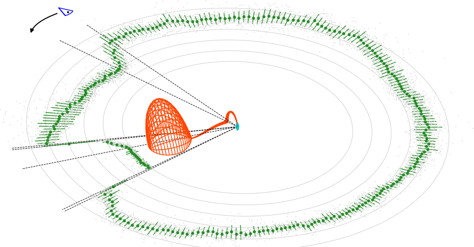
Figure 11: A three dimensional view into the system geometry. Central in the figure are shown the white dwarf (cyan), the donor star (orange wireframe) and the accretion stream. A radial projection of the average phase-folded light curve of J0614–27 is plotted in green. The phase regions corresponding to those marked in the bottom panel of Figure 6 (also Table 4) are delineated by the dashed black lines emanating from the WD along the line of sight to the observer. In the co-rotating reference frame of the binary, the observer would move in a counter-clockwise direction around the center of mass. This figure shows how the features in the light curve correspond to the physical components of the system.

9 Conclusions

In this paper we have reported on the discovery, observations, and modelling of a new eclipsing magnetic cataclysmic variable, MASTER OT J061451.70–272535.5. By modelling the light curve with a modified genetic algorithm based on the “firefly” model of Hakala et al. (2002), we constrain the inclination and mass ratio of the system and subsequently derive the binary orbital parameters.

In the context of stellar evolution, eclipsing polars such as J0614–27 play a particularly important role. There is by now significant evidence that the evolutionary pathway for mCVs is distinct from that of non-magnetic CVs, perhaps the most conspicuous being the reduced importance of the $2-3\,$h period gap (see Figure 1). The period of J0614–27 nearly coincides with the lower edge of the period gap - a time in the evolution when the donor star is re-establishing contact with its Roche lobe after being in a prolonged (multi-million year) low-mass-transfer state. The system parameters suggest that J0614–27 is most probably evolving to shorter periods, rather than being a post-bounce system, and could therefore be valuable in helping constrain evolutionary scenarios, particularly w.r.t. the efficacy of residual magnetic breaking within the period gap. We therefore conclude by recommending J0614–27 as a worthy candidate for further multi-wavelength (particularly X-ray) follow up observations in order to shed light on the remaining uncertainties concerning the accretion flow, magnetic field structure, and evolutionary status of MASTER OT J061451.70–272535.5.

References

- Bailey & Cropper (1991) Bailey J., Cropper M., 1991, MNRAS, 253, 27
- Beardmore et al. (1995) Beardmore A. P., Ramsay G., Osborne J. P., Mason K. O., Nousek J. A., Baluta C., 1995, MNRAS, 273, 742
- Belle et al. (2002) Belle K. E., Howell S. B., Sirk M. M., Huber M. E., 2002, ApJ, 577, 359
- Beuermann (2004) Beuermann K., 2004, in International Astronomical Union Colloquium. Cambridge University Press (arXiv:astro-ph/0302235), doi:10.1017/S0252921100002098
- Beuermann et al. (2007) Beuermann K., Euchner F., Reinsch K., Jordan S., Gänsicke B. T., 2007, A&A, 463, 647
- Bradley et al. (2016) Bradley L., et al., 2016, astropy/photutils: v0.3, doi:10.5281/zenodo.164986, https://doi.org/10.5281/zenodo.164986
- Bridge et al. (2003) Bridge C. M., Cropper M., Ramsay G., de Bruijne J. H. J., Reynolds A. P., Perryman M. A. C., 2003, MNRAS, 341, 863
- Bridge et al. (2004) Bridge C. M., Hakala P., Cropper M., Ramsay G., 2004, MNRAS, 351, 1423
- Buckley et al. (1998) Buckley D. A. H., Barrett P. E., Haberl F., Sekiguchi K., 1998, MNRAS, 299, 998
- Buckley et al. (2006) Buckley D. A. H., Swart G. P., Meiring J. G., 2006, in Society of Photo-Optical Instrumentation Engineers (SPIE) Conference Series. p. 62670Z, doi:10.1117/12.673750
- Buckley et al. (2008) Buckley D. A. H., et al., 2008, in Ground-based and Airborne Instrumentation for Astronomy II. p. 701407, doi:10.1117/12.789438
- Burgh et al. (2003) Burgh E. B., Nordsieck K. H., Kobulnicky H. A., Williams T. B., O’Donoghue D., Smith M. P., Percival J. W., 2003, in Iye M., Moorwood A. F. M., eds, Proc. SPIEVol. 4841, Instrument Design and Performance for Optical/Infrared Ground-based Telescopes. pp 1463–1471, doi:10.1117/12.460312
- Chanan et al. (1976) Chanan G. A., Middleditch J., Nelson J. E., 1976, ApJ, 208, 512
- Coppejans et al. (2013) Coppejans R., et al., 2013, PASP, 125, 976
- Crawford et al. (2010) Crawford S. M., et al., 2010, in Observatory Operations: Strategies, Processes, and Systems III. p. 773725, doi:10.1117/12.857000
- Cropper (1990) Cropper M., 1990, Space Sci. Rev., 54, 195
- Denisenko & Martinelli (2016) Denisenko D. V., Martinelli F., 2016, arXiv e-prints, p. arXiv:1609.08511
- Drake et al. (2009) Drake A. J., et al., 2009, ApJ, 696, 870
- Drake et al. (2014) Drake A. J., et al., 2014, ApJS, 213, 9
- Ferrario et al. (2015a) Ferrario L., de Martino D., Gänsicke B. T., 2015a, Space Sci. Rev., 191, 111
- Ferrario et al. (2015b) Ferrario L., de Martino D., Gänsicke B. T., 2015b, Space Science Reviews, 191, 111
- Fuchs et al. (2016) Fuchs J. T., et al., 2016, MNRAS, 462, 2382
- Hakala (1995) Hakala P. J., 1995, A&A, 296, 164
- Hakala et al. (1994) Hakala P. J., Piirola V., Vilhu O., Osborne J. P., Hannikainen D. C., 1994, MNRAS, 271, L41
- Hakala et al. (2002) Hakala P., Cropper M., Ramsay G., 2002, MNRAS, 334, 990
- Harrop-Allin et al. (1999) Harrop-Allin M. K., Cropper M., Hakala P. J., Hellier C., Ramseyer T., 1999, MNRAS, 308, 807
- Hellier (2001) Hellier C., 2001, Cataclysmic Variable Stars. Springer Science & Business Media
- Hong et al. (2012) Hong J., van den Berg M., Grindlay J. E., Servillat M., Zhao P., 2012, ApJ, 746, 165
- King & Williams (1985) King A. R., Williams G. A., 1985, MNRAS, 215, 1P
- Kniazev et al. (2004) Kniazev A. Y., Pustilnik S. A., Grebel E. K., Lee H., Pramskij A. G., 2004, ApJS, 153, 429
- Kniazev et al. (2008) Kniazev A. Y., et al., 2008, MNRAS, 388, 1667
- Knigge et al. (2011) Knigge C., Baraffe I., Patterson J., 2011, ApJS, 194, 28
- Kohonen (1990) Kohonen T., 1990, Proceedings of the IEEE, 78, 1464
- Kornilov et al. (2012) Kornilov V. G., et al., 2012, Experimental Astronomy, 33, 173
- Kuijpers & Pringle (1982) Kuijpers J., Pringle J. E., 1982, A&A, 114, L4
- Lipunov et al. (2010) Lipunov V., et al., 2010, Advances in Astronomy, 2010, 349171
- Lipunov et al. (2016) Lipunov V., et al., 2016, in Revista Mexicana de Astronomia y Astrofisica Conference Series. pp 42–47
- Littlefield et al. (2015) Littlefield C., et al., 2015, MNRAS, 449, 3107
- Lomb (1976) Lomb N. R., 1976, Ap&SS, 39, 447
- Long et al. (2012) Long M., Romanova M. M., Lamb F. K., 2012, New Astron., 17, 232
- Masetti et al. (2013) Masetti N., et al., 2013, A&A, 556, A120
- Mason (2004) Mason P. A., 2004, in Tovmassian G., Sion E., eds, Revista Mexicana de Astronomia y Astrofisica, vol. 27 Vol. 20, Revista Mexicana de Astronomia y Astrofisica Conference Series. pp 180–181
- Mason et al. (1998) Mason P. A., Ramsay G., Andronov I., Kolesnikov S., Shakhovskoy N., Pavlenko E., 1998, MNRAS, 295, 511
- McAllister et al. (2017) McAllister M. J., et al., 2017, Monthly Notices of the Royal Astronomical Society, 464, 1353
- Mouchet et al. (2017) Mouchet M., et al., 2017, A&A, 600, A53
- Mukai (2017) Mukai K., 2017, PASP, 129, 062001
- Nauenberg (1972) Nauenberg M., 1972, ApJ, 175, 417
- O’Donoghue et al. (2006) O’Donoghue D., et al., 2006, MNRAS, 372, 151
- Patterson (1994) Patterson J., 1994, PASP, 106, 209
- Patterson et al. (1981) Patterson J., Williams G., Hiltner W. A., 1981, ApJ, 245, 618
- Patterson et al. (1995) Patterson J., Skillman D. R., Thorstensen J., Hellier C., 1995, Publications of the Astronomical Society of the Pacific, 107, 307
- Ramsay & Cropper (2002) Ramsay G., Cropper M., 2002, MNRAS, 335, 918
- Ramsay & Cropper (2003) Ramsay G., Cropper M., 2003, MNRAS, 338, 219
- Ramsay et al. (2004) Ramsay G., Cropper M., Mason K. O., Córdova F. A., Priedhorsky W., 2004, MNRAS, 347, 95
- Ritter & Kolb (2003) Ritter H., Kolb U., 2003, A&A, 404, 301
- Rojas et al. (2017) Rojas A. F., et al., 2017, A&A, 602, A124
- Rosen et al. (1996) Rosen S. R., et al., 1996, MNRAS, 280, 1121
- Rosner (1983) Rosner B., 1983, Technometrics, 25, 165
- Salvi et al. (2002) Salvi N., Ramsay G., Cropper M., Buckley D. A. H., Stobie R. S., 2002, MNRAS, 331, 488
- Scargle (1982) Scargle J. D., 1982, ApJ, 263, 835
- Schmidt et al. (1999) Schmidt G. D., Hoard D. W., Szkody P., Melia F., Honeycutt R. K., Wagner R. M., 1999, ApJ, 525, 407
- Schmidt et al. (2005) Schmidt G. D., et al., 2005, ApJ, 620, 422
- Schwarz et al. (2002) Schwarz R., Greiner J., Tovmassian G. H., Zharikov S. V., Wenzel W., 2002, A&A, 392, 505
- Schwope et al. (1993) Schwope A. D., Thomas H. C., Beuermann K., 1993, A&A, 271, L25
- Schwope et al. (1995) Schwope A. D., Thomas H.-C., Beuermann K., Burwitz V., Jordan S., Haefner R., 1995, A&A, 293, 764
- Schwope et al. (1997) Schwope A. D., Mantel K. H., Horne K., 1997, A&A, 319, 894
- Schwope et al. (2015) Schwope A. D., Mackebrandt F., Thinius B. D., Littlefield C., Garnavich P., Oksanen A., Granzer T., 2015, Astronomische Nachrichten, 336, 115
- Shumkov et al. (2015) Shumkov V., et al., 2015, The Astronomer’s Telegram, 7127
- Sirk & Howell (1998) Sirk M. M., Howell S. B., 1998, ApJ, 506, 824
- Spark & O’Donoghue (2015) Spark M. K., O’Donoghue D., 2015, MNRAS, 449, 175
- Stickel (2010) Stickel J. J., 2010, Computers & Chemical Engineering, 34, 467
- Szkody (1998) Szkody P., 1998, in Howell S., Kuulkers E., Woodward C., eds, Astronomical Society of the Pacific Conference Series Vol. 137, Wild Stars in the Old West. p. 18
- Traulsen et al. (2010) Traulsen I., Reinsch K., Schwarz R., Dreizler S., Beuermann K., Schwope A. D., Burwitz V., 2010, A&A, 516, A76
- VanderPlas & Ivezić (2015) VanderPlas J. T., Ivezić Ž., 2015, ApJ, 812, 18
- Vanderplas (2015) Vanderplas J., 2015, gatspy: General tools for Astronomical Time Series in Python, doi:10.5281/zenodo.14833, https://doi.org/10.5281/zenodo.14833
- Wang et al. (2017) Wang S., Bai Y., Zhang C.-P., Liu J.-F., 2017, Research in Astronomy and Astrophysics, 17, 10
- Warner (2003) Warner B., 2003, Cataclysmic Variable Stars. Cambridge University Press, doi:10.1017/CB0978O511586491
- Watson et al. (1989) Watson M. G., King A. R., Jones M. H., Motch C., 1989, MNRAS, 237, 299
- Wynn & King (1995) Wynn G. A., King A. R., 1995, MNRAS, 275, 9
- Zdziarski et al. (2016) Zdziarski A. A., Ziółkowski J., Bozzo E., Pjanka P., 2016, A&A, 595, A52
- Zhilkin et al. (2012) Zhilkin A. G., Bisikalo D. V., Mason P. A., 2012, Astronomy Reports, 56, 257
- Zhilkin et al. (2016) Zhilkin A. G., Bisikalo D. V., Mason P. A., 2016, in American Institute of Physics Conference Series. p. 020002, doi:10.1063/1.4942564
- Zorotovic et al. (2011) Zorotovic M., Schreiber M. R., Gänsicke B. T., 2011, A&A, 536, A42
- de Martino et al. (2001) de Martino D., et al., 2001, A&A, 377, 499
- de Martino et al. (2004) de Martino D., Matt G., Belloni T., Haberl F., Mukai K., 2004, A&A, 415, 1009