On static chiral Milton-Briane-Willis continuum mechanics

Abstract

Recent static experiments on twist effects in chiral three-dimensional mechanical metamaterials have been discussed in the context of micropolar Eringen continuum mechanics, which is a generalization of Cauchy elasticity. For cubic symmetry, Eringen elasticity comprises nine additional parameters with respect to Cauchy elasticity, of which three directly influence chiral effects. Here, we discuss the behavior of the static case of an alternative generalization of Cauchy elasticity, the Milton-Briane-Willis equations. We show that in the homogeneous static cubic case only one additional parameter with respect to Cauchy elasticity results, which directly influences chiral effects. We show that the Milton-Briane-Willis equations qualitatively describe the experimentally observed chiral twist effects, too. We connect the behavior to a characteristic length scale.

I 1. Introduction

In one dimension, the scalar spring constant in Hooke’s law connects forces and displacements. As a generalization towards three-dimensional continuum mechanics Banerjee (2011), the rank-4 Cauchy elasticity tensor, ${\bf\bm{C}}$, connects the rank-2 stress tensor, $\bm{\sigma}$, and the rank-2 strain tensor, $\bm{\epsilon}$. In general, Cauchy elasticity comprises up to 21 independent nonzero parameters describing possible linear deformations of elastic bodies in three dimensions Sommerfeld (1950); Authier (2003); Milton (2002); Milton et al. (2016); Laude (2015). For cubic crystals, which are characterized by four three-fold rotational axes, only 3 parameters remain Authier (2003).

However, Cauchy elasticity essentially only grasps the displacements, $\bm{u}(\bm{r}),$ of infinitesimally small volume elements (of “points”) within a fictitious continuum. Cauchy elasticity therefore misses certain degrees of freedom in artificial three-dimensional periodic microlattices or metamaterials, for which the unit cell has a finite extent rather than being approximately point-like such as atoms in an ordinary crystal of macroscopic size Frenzel et al. (2017); Rueger and Lakes (2018). Such missed degrees of freedom have recently become particularly obvious in chiral three-dimensionally periodic mechanical metamaterial structures (see Fig. 1(a)) for which Cauchy elasticity fails to describe any effect of chirality, whereas prominent twist effects have been observed experimentally in the static case Frenzel et al. (2017). In contrast, micropolar Eringen elasticity (see Fig. 1(b)) has been able to describe these experimental findings Frenzel et al. (2017) as well as others for achiral media Rueger and Lakes (2018). Cosserat elasticity Eringen (1974) can be seen as a special case of Eringen micropolar elasticity.

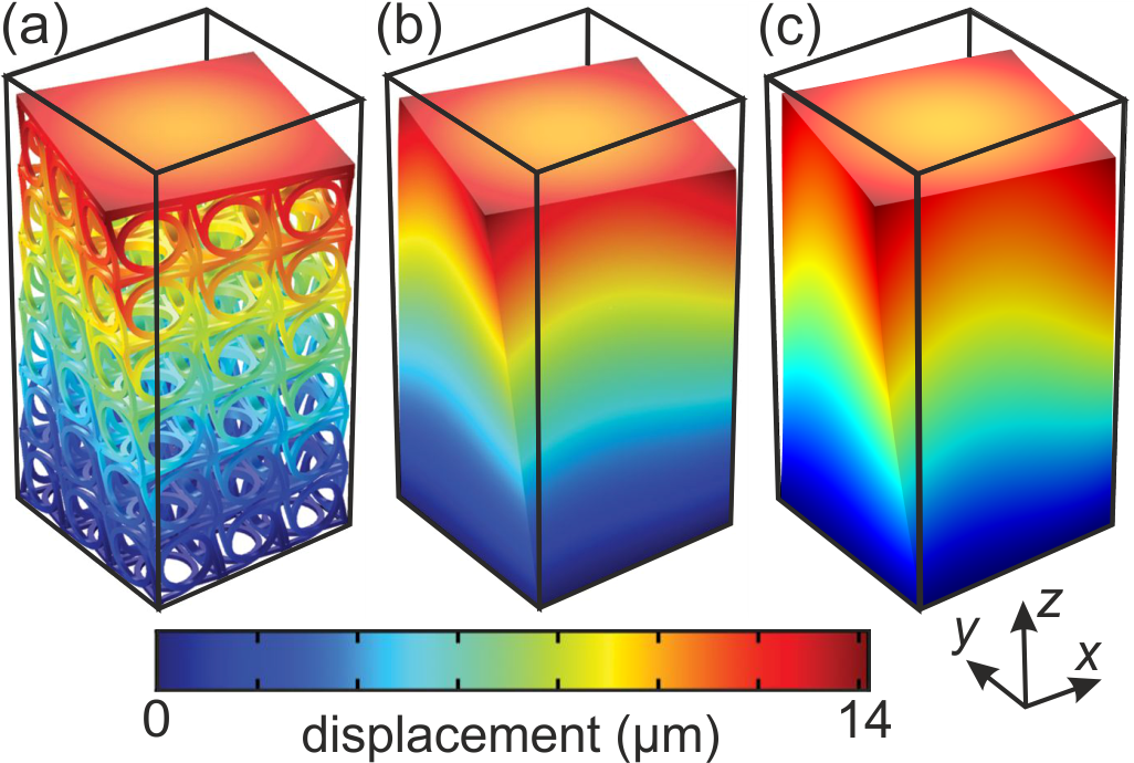
Figure 1: Cuboid beams with volume $L\times L\times 2L$, with side length $L=500\ \mathrm{\mu m}$, are subject to uniaxial loading along the negative $z$-direction. In Cauchy elasticity, the beam compresses and can expand or contract laterally, depending on its Poisson ratio (not depicted). However, a twist is forbidden in Cauchy elasticity, even if the underlying crystal symmetry would allow for a twist. (a) Finite-element calculation for a chiral metamaterial microstructure exhibiting a twist behavior Frenzel et al. (2017). (b) Same as (a), but calculated using chiral micropolar Eringen elasticity Frenzel et al. (2017). Panels (a) and (b) are taken with permission from Frenzel et al. (2017). (c) Numerical calculations based on generalized Cauchy elasticity following Milton-Briane-Willis. For all three panels, the effects are calculated within the linear elastic regime and are magnified tenfold for clarity. The modulus of the displacement vector field is superimposed on a false-color scale. Parameters in (c) are: $C_{11}=32.8\;\rm MPa$, $C_{12}=-6.1\;\rm MPa$, $C_{44}=19.4\;\rm MPa$ (in Voigt notation), and $\alpha=3\;\rm GPa/m$.

Cosserat elasticity, micropolar Eringen elasticity Bigoni and Drugan (2007), micromorphic Eringen elasticity Eringen (1974); Toupin (1964), strain-gradient theories Gudmundson (2004), and yet more advanced approaches Seppecher et al. (2011) are not the only possible generalizations of Cauchy elasticity though. It is therefore interesting and relevant to ask which generalizations other than Eringen’s can describe the effects of chirality observed in recent experiments Frenzel et al. (2017).

In this paper, in Section 2., we start with the static version of a generalization of Cauchy elasticity following Milton, Briane, and Willis Milton et al. (2006). This generalization arises from demanding that the resulting equations are mathematically form invariant under coordinate transformations. Aiming at describing recent experiments Frenzel et al. (2017), we focus on the case of three-dimensional homogeneous cubic crystals without centrosymmetry, in which case the terms beyond Cauchy elasticity can be parameterized by a single scalar parameter. In Section 3., we discuss numerical solutions. We find that the resulting behavior qualitatively describes the push-to-twist conversion effects observed in recent experiments (see Fig. 1(c)) and that it can be connected to a characteristic length scale. We conclude in Section 4.

II 2. Generalized Static Cauchy elasticity

In the static case, all forces must balance. For simplicity, we omit external forces in all formulas throughout this paper; we implement them via boundary conditions. Hence, the divergence of the stress tensor $\bm{\sigma}=\bm{C}:\ \bm{\epsilon}$ is zero, ${\bm{\nabla}}\cdot\bm{\sigma}=\bm{0}$. The symbol “:” denotes a double contraction, the dot “$\cdot$” denotes a contraction between two tensors. Cauchy elasticity reduces to the compact equation

$${\bm{\nabla}}\cdot\left(\bm{C}:\bm{\epsilon}\ \right)=\bm{0},$$ (1)

where $\bm{C}$ is the rank-4 elasticity tensor, with components $C_{ijkl}$ ($i,j,k,l=1,2,3$) in Cartesian coordinates and S.I. units of $\mathrm{Pa}$, and $\bm{\epsilon}$ is the dimensionless symmetric rank-2 strain tensor with components ${\epsilon}_{ij}={\epsilon}_{ji}$ Sommerfeld (1950). The strain tensor can be connected to the gradient of the displacement vector field $\bm{u}=\bm{u}(\bm{r})$ with components ${u}_{i}$ ($i=1,2,3$) via Sommerfeld (1950)

$$\bm{\epsilon}=\frac{1}{2}\left({\bm{\nabla}}\bm{u}+{\left({\bm{\nabla}}\bm{u}\right)}^{\mathrm{T}}\right),$$ (2)

where the superscript “T” refers to the transposed quantity. The Cauchy elasticity tensor obeys the minor symmetries (${\mathop{C}}_{ijkl}=C_{jikl}=C_{ijlk}$) and the major symmetries ($C_{ijkl}=C_{klij}$) Sommerfeld (1950). As a result, the strain tensor $\bm{\epsilon}$ in (1) can equivalently be replaced by the gradient of the displacement vector $\bm{\nabla}\bm{u}$, i.e.,

$${\bm{\nabla}}\cdot\left(\bm{C}:\bm{\nabla}\bm{u}\ \right)=\bm{0}\,.$$ (3)

Cauchy elasticity does not describe effects of chirality at all Eringen (1974). This fact can immediately be seen by recalling that all even-rank tensors (such as the rank-2 stress tensor, the rank-4 elasticity stress tensor, and the rank-2 strain tensor) are invariant under space inversion operations, $\bm{r}\to-\bm{r}$ Eringen (1974). Thus, (3) does not change under space inversion, which brings one from a left-handed to a right-handed medium (or vice versa).

A space inversion is a special example of a general spatial coordinate transformation $\bm{r}\to{\bm{r}^{\prime}}\left(\bm{r}\right)$. It has first been pointed out by Milton, Briane, and Willis Milton et al. (2006) in 2006 that Cauchy elasticity is not form invariant under general curvilinear coordinate transformations (also see Brun et al. (2009); Norris and Shuvalov (2011); Diatta and Guenneau (2014)). This finding is disturbing in view of the fact that most other equations in physics such as, for example, the quantum mechanical Schrödinger equation, the wave equation of longitudinal pressure waves in gases/fluids, the time-dependent Maxwell equations, Fourier’s time-dependent heat conduction equation, Fick’s stationary diffusion equation, the stationary electric conduction equation, and the stationary laminar fluid-flow equation are form invariant under coordinate transformations Dolin (1961); Leonhardt (2006); Pendry et al. (2006); Milton et al. (2006); Cummer and Schurig (2007); Brun et al. (2009); Norris and Shuvalov (2011); Kadic et al. (2012); Guenneau et al. (2012); Guenneau and Puvirajesinghe (2013); McCall et al. (2018). Milton, Briane, and Willis arrived at a generalization of dynamic Cauchy elasticity that is form invariant under coordinate transformations Milton et al. (2006). In the static limit, i.e., for angular frequency $\omega=0$ and finite static mass density $\rho$, their equation (2.4) reduces to

$${\bm{\nabla}}\cdot\left(\bm{C}:{\bm{\nabla}}\bm{u}+\bm{S}\cdot\bm{u}\right)-\bm{D}:{\bm{\nabla}}\bm{u}=\bm{0},$$ (4)

where $\bm{C}=\bm{C}(\bm{r})$ and the two additional rank-3 tensors $\bm{S}=\bm{S}(\bm{r})$ and $\bm{D}=\bm{D}(\bm{r})$ generally depend on the spatial position $\bm{r}$.

In the case of a homogeneous material or homogenized structure with ${\bm{\nabla}}S_{ijk}={\bm{\nabla}}D_{ijk}=\bm{0}$, which is the focus of interest in this paper, equation (4) reduces to

$$\bm{\nabla}\cdot\left(\bm{C}:{\bm{\nabla}}\bm{u}\ +\bm{W}\cdot\bm{u}\right)=\bm{0},$$ (5)

with the rank-3 tensor $\bm{W}$ defined by

$$\bm{W}=\bm{S}-\bm{D}^{\mathrm{T}},$$ (6)

where the components of the “transposed” tensor are given by

$$D^{\mathrm{T}}_{ijk}=D_{jik}.$$ (7)

Broken centrosymmetry is a necessary requirement for chirality Eringen (1974); Authier (2003); Frenzel et al. (2017). If we nevertheless consider an isotropic medium or a cubic crystal with centrosymmetry, it follows that $\bm{W}\equiv\bm{0}$, just like for any homogeneous rank-3 tensor Authier (2003). $\bm{W}\equiv\bm{0}$ also holds true for an isotropic medium without centrosymmetry.

For a cubic crystal without centrosymmetry, we find that the tensor $\bm{W}$, such as any rank-3 tensor Authier (2003), reduces to the rank-3 Levi-Civita tensor ${\bm{\varepsilon}}$ (with components ${{\varepsilon}}_{123}={\mathrm{\varepsilon}}_{231}={\mathrm{\varepsilon}}_{312}=-{\mathrm{\varepsilon}}_{132}=-{\mathrm{\varepsilon}}_{213}=-{\mathrm{\varepsilon}}_{321}=1$, all other components are zero) times a scalar factor $\alpha$, i.e.,

$$\bm{W}=\alpha\,\bm{\varepsilon}.$$ (8)

$\alpha$ has S.I. units of $\mathrm{Pa/m}$. This allows us to rewrite Milton-Briane-Willis elasticity (5) to

$$\bm{\nabla}\cdot\left(\bm{C}:\ \bm{\nabla}\bm{u}\right)-\alpha\ \bm{\nabla}\times\bm{u}=\bm{0}.$$ (9)

It is instructive to investigate the behavior of (9) under a space inversion operation, $\bm{r}\to-\bm{r}$. As argued below (3), $\bm{C}:\bm{\nabla}\bm{u}=\bm{C}:\bm{\epsilon}$ does not change sign, but the $\bm{\nabla}$ in front does. In the second term in (9), both $\bm{\nabla}$ and $\bm{u}$ do change sign, hence the vector product does not change sign. Therefore, the relative sign of the first and second term in (9) changes when performing a space inversion. Thus, (9) is different for a left- and a right-handed medium, respectively. This behavior is a necessary condition for a continuum formulation to be able to describe the effects of chirality in mechanics. Clearly, if the single parameter beyond Cauchy elasticity is zero, $\alpha=0$, equation (9) reduces to Cauchy elasticity (3). As usual Authier (2003); Banerjee (2011), for cubic symmetry (with or without a center of inversion), the Cauchy elasticity tensor $\bm{C}$ contains $3$ independent nonzero scalar parameters Authier (2003).

We will use (9) for the numerical calculations presented in Section 3. To be unambiguous and clear for experimentalists, we therefore write equation (9) out into its three components and explicitly write out all involved sums, leading to

$$\sum^{3}_{i,k,l=1}{\left(\frac{\partial}{\partial x_{i}}\left(C_{i1kl}\frac{\partial u_{l}}{\partial x_{k}}\right)\right)}-\alpha\left(\frac{\partial u_{3}}{\partial x_{2}}-\frac{\partial u_{2}}{\partial x_{3}}\right)=0,\,\,\,\,\,\,\,\,\,$$ (10)

$$\sum^{3}_{i,k,l=1}{\left(\frac{\partial}{\partial x_{i}}\left(C_{i2kl}\frac{\partial u_{l}}{\partial x_{k}}\right)\right)}-\alpha\left(\frac{\partial u_{1}}{\partial x_{3}}-\frac{\partial u_{3}}{\partial x_{1}}\right)=0,\,\,\,\,\,\,\,\,\,$$ (11)

and

$$\sum^{3}_{i,k,l=1}{\left(\frac{\partial}{\partial x_{i}}\left(C_{i3kl}\frac{\partial u_{l}}{\partial x_{k}}\right)\right)}-\alpha\left(\frac{\partial u_{2}}{\partial x_{1}}-\frac{\partial u_{1}}{\partial x_{2}}\right)=0.\,\,\,\,\,\,\,\,\,$$ (12)

III 3. Numerical calculations

In what follows, we illustrate the generalized static homogeneous equation (9) for a cubic three-dimensional chiral medium by example numerical calculations. To allow for a direct comparison with micropolar Eringen elasticity, we reproduce previous continuum results Frenzel et al. (2017) and results of metamaterial microstructure calculations Frenzel et al. (2017) at selected points for convenience of the reader. To ease this comparison, we also choose similar parameters as much as possible.

III.1 3.1 Numerical approach

In our numerical calculations, we consider cuboid shaped samples with volume $L\times L\times 2L$. We apply uniaxial loading by a rigid stamp along the negative $z$-direction with sliding boundary conditions at the top, i.e., at the top surface we have the displacement $\bm{u}={\left(0,0,u_{z}\right)}^{\mathrm{T}}$ with $u_{z}\neq 0$. The axial strain results from $\epsilon=\epsilon_{33}=-u_{z}/L$. The uniaxial pressure, $P$, exerted at the top is given by $P={\bm{n}}\;\mathrm{\cdot}\;\mathrm{(}\bm{C}\;\mathrm{:}\;\bm{\nabla}\bm{u}-\alpha\ \bm{\nabla}\times\bm{u}\mathrm{)}$, where ${\bm{n}}$ is the normal vector pointing into the negative $z$-direction. On the four sides we use open boundary conditions, i.e., ${\bm{n}}\;\mathrm{\cdot}\left(\bm{C}\;\mathrm{:}\;\bm{\nabla}\bm{u}-\alpha\ \bm{\nabla}\times\bm{u}\right)\mathrm{=0}$, with the respective normal vectors ${\bm{n}}$ of the four side facets. On the bottom of the cuboid, we use fixed boundary conditions with $\bm{u}={\left(0,0,0\right)}^{\mathrm{T}}$, describing that the sample cuboid is fixed to a substrate. We have used the same conceptual boundary conditions in our previous work on static Eringen elasticity Frenzel et al. (2017).

We solve equation (9) by using a finite-element approach via the partial differential equation (PDE) module of the commercial software package COMSOL Multiphysics. Herein, the homogeneous sample cuboid is typically discretized into $10^{4}$ tetrahedra, corresponding to about $5\times 10^{4}$ degrees of freedom. Finer discretization has led to negligible changes with respect to the results outlined in the following.

In Section 3.2., we will discuss the behavior of the twist angle and the axial strain of the cuboid sample under uniaxial loading. The axial strain is defined as the $z$-component of the displacement vector at the top surface (which is the same for all positions ${\left(x,y,2L\right)}^{\mathrm{T}}$), divided by the sample length $2L$, i.e., by $u_{z}(x,y,2L)/(2L)$.

The twist angle is defined via the displacement of the equivalent four corners at the top of the sample cuboid in the $xy$-plane, which are at positions ${\left(\pm L/2,\pm L/2,2L\right)}^{\mathrm{T}}$ before loading, with respect to the sample center at ${\left(0,0,2L\right)}^{\mathrm{T}}$. For pure twists without further deformations, this definition grasps the entire sample behavior. If deformations that are more complex occur in addition, the twist angle resulting from our definition should be seen as merely a parameter representing part of the overall behavior.

III.2 3.2 Results and discussion

Figure 1 shows the modulus of the displacement vector field (on a false-color scale) for uniaxial loading along the negative $z$-axis of a cuboid shaped sample with volume $L\times L\times 2L$. All results shown are within the linear elastic regime, i.e., for axial strains $<1\%$. We choose $L=500\,\rm\mu m$ (see $N=1$ in Frenzel et al. (2017)), $C_{11}=C_{22}=C_{33}$ (in standard Voigt notation Eringen (1974)), $C_{12}=C_{13}=C_{21}=C_{23}=C_{31}=C_{32}$, $C_{44}=C_{55}=C_{66}$ (all other elements of the elasticity tensor are zero), and $\alpha=3\,$GPa/m.

The results of Milton-Briane-Willis generalized Cauchy elasticity in Fig. 1(c) are compared with those of micropolar Eringen elasticity Frenzel et al. (2017) in panel (b) and finite-element metamaterial microstructure calculations Frenzel et al. (2017) in panel (a). For the details underlying panels (a) and (b), we refer the reader to the extensive discussion in Frenzel et al. (2017) and the corresponding supporting online material. Obviously, Milton-Briane-Willis generalized Cauchy elasticity, micropolar Eringen elasticity, and the finite-element microstructure calculations exhibit the same qualitative behavior. When replacing $\alpha\to-\alpha$, the direction of the twist changes from clockwise to counter-clockwise in Figs. 1(b) and (c) (not depicted), corresponding to the behavior of the mirror image of the 3D microstructure shown in Fig. 1(a).

In Figure 2(a), the parameters are the same as in Fig. 1(c), except that we consider the three choices (a) $\alpha=3\,$GPa/m, (b) $\alpha\to 3.3\,\alpha$, and (c) $\alpha\to 33\,\alpha$. In Fig. 2(b), the twist effect is simply larger than that in panel (a). In panel (c), however, unusual additional substructures appear in the displacement field.

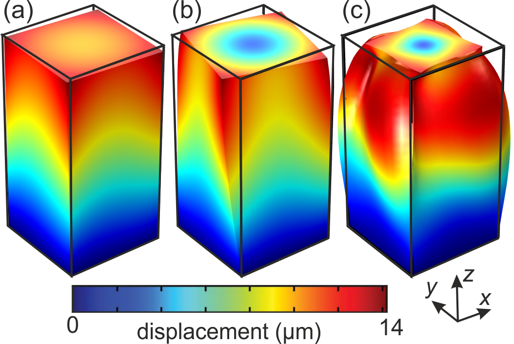
Figure 2: (a) Same as Fig. 1(c) with parameter $\alpha=3\;$GPa/m and all other parameters fixed as in Fig. 1(c). (b) $\alpha\to 3.3\;\alpha$. (c) $\alpha\to 33\;\alpha$. From such raw data, the twist angle at the top per axial strain can be deduced and plotted versus $\alpha$ (see Fig. 3). All deformations are magnified twofold for clarity.

Figure 3 emphasizes essentially the same aspect as Fig. 2, however, we do not depict displacement fields of a sample but rather plot the calculated twist/strain (defined in Section 3.1.) versus the parameter $\alpha$ for fixed sample side length $L$. For small values of $\alpha$, the twist/strain increases monotoneously. However, for larger values of $\alpha$, we find an unusual non-monotoneous resonance-like behavior (compare Milton and Willis (2007)), which is connected to the behavior shown in Fig. 2(c).

This behavior versus the parameter $\alpha$ for fixed sample side length $L$ is connected to the behavior versus $L$ for fixed $\alpha$. Following references Eringen (1974); Frenzel et al. (2017), the effects beyond static Cauchy elasticity should decrease with increasing $L$. More specifically, the twist/strain should decrease proportional to the surface-to-volume ratio, i.e., decrease $\propto 1/L$. What one gets from (9) versus $L$ for fixed $\alpha$ is the polar opposite of this behavior. This can be seen as follows: If we replace the spatial components $x_{i}\rightarrow\zeta x_{i}$ in (9), with some dimensionless scaling factor $\zeta$, the ratio of the second and first term in (9) increases by factor $\zeta$. This means that the effects beyond Cauchy elasticity would increase with increasing sample side length $L$ if $\alpha$ was constant. We conclude that $\alpha$ must not be considered as a constant material parameter, but rather as an effective continuum-model parameter.

To arrive at a meaningful material parameter, $\beta$, we make the ansatz

$$\alpha=\frac{\beta}{L^{2}}\ .$$ (13)

The parameter $\beta$ has S.I. units of $\mathrm{Pa}\,\mathrm{m}$. Thus, the ratio

$$l_{\mathrm{c}}=\frac{\beta}{C}$$ (14)

has units of a length. Here, $C$ is a nonzero element of the elasticity tensor $\bm{C}$ or a combination of elements. As the twist effect mainly changes the shape of the specimen but not its volume, we choose the shear modulus $C=C_{44}=C_{2323}$. The length $l_{\mathrm{c}}$ is obviously zero in the Cauchy limit of $\alpha=\beta=0$. Therefore, it is tempting to interpret $l_{\mathrm{c}}$ as a characteristic length scale in the same spirit as characteristic length scales in micropolar Eringen elasticity Eringen (1974). There, one gets several different characteristic length scales, all of which are zero in the Cauchy limit.

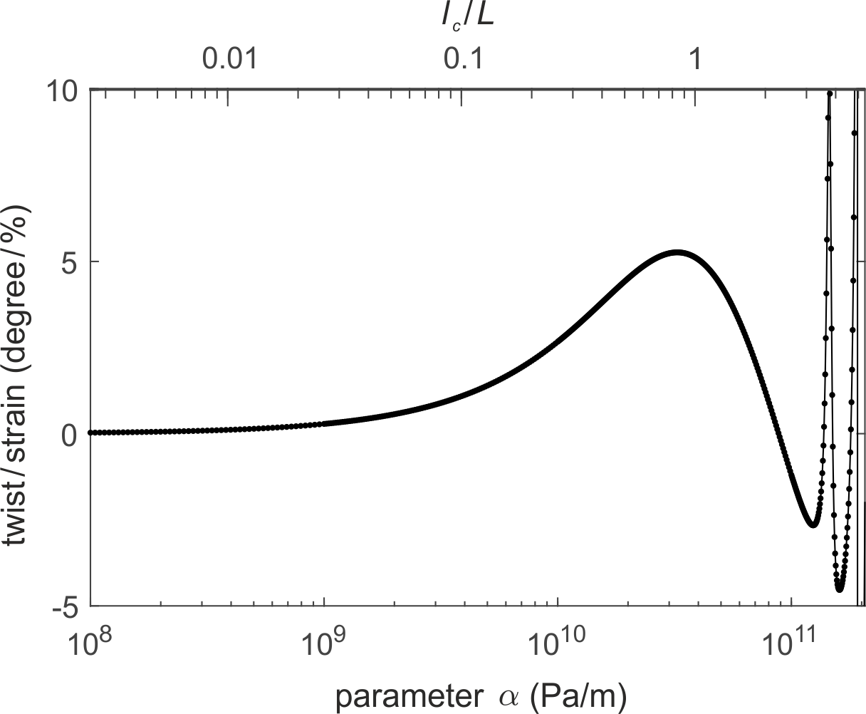
Figure 3: Twist/strain versus parameter $\alpha$ (lower horizontal scale) as deduced from raw data such as the ones shown in Fig. 2. The dots are calculated, the curve is a guide to the eye. Parameters are as in Fig. 1(c). The upper horizontal scale shows the characteristic length $l_{\mathrm{c}}$ normalized to the sample side length $L$, $\frac{l_{\mathrm{c}}}{L}=\frac{\beta/C_{44}}{L}=\alpha\frac{L}{C_{44}}$ according to (15). Here, $C_{44}$ is an element of the elasticity tensor in Voigt notation, namely the shear modulus $C_{2323}$.

To test this ansatz for the characteristic length scale, we depict as the upper horizontal scale in Fig. 3 the normalized characteristic length, $l_{\mathrm{c}}/L$, which follows from

$$\frac{l_{\mathrm{c}}}{L}=\frac{\beta/C_{44}}{L}=\alpha\frac{L}{C_{44}}.$$ (15)

We find that non-monotoneous behavior in Fig. 3 occurs when $l_{\rm c}$ becomes comparable to or even exceeds the sample side length $L$. Likewise, the characteristic length $l_{\mathrm{c}}=1275\,\rm\mu m$ in Fig. 2(c) is also larger than the sample side length of $L=500\,\rm\mu m$, whereas $l_{\rm c}$ is smaller by factor $33$ and $10$, respectively, in panels (a) and (b).

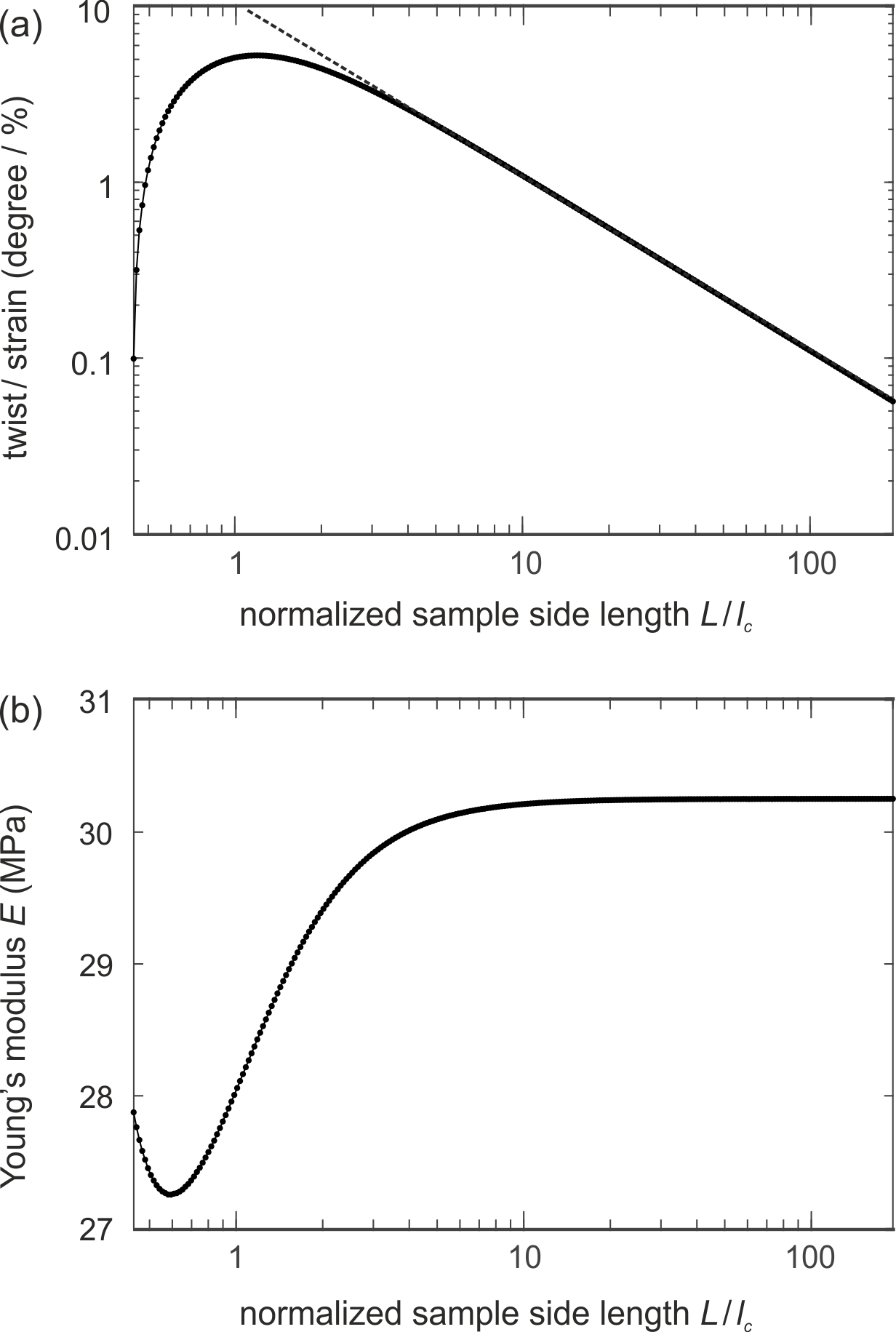
Figure 4: (a) Twist/strain versus sample side length $L$ normalized by the characteristic length $l_{\rm c}$ on a double logarithmic scale. The dependence on the parameter $\beta$ is implicitly contained in this normalization. The dashed straight line has a slope of $-1$ corresponding to the expected asymptotic scaling of the twist angle $\propto 1/L$ for fixed parameter $\beta$. (b) Same as in (a) but for the effective Young’s modulus $E$ on a semi-logarithmic scale. All other parameters are as in Fig. 1(c). The dots are calculated, the curves are guides to the eye.

Finally, we study the dependence of the behavior on the sample side length $L$ for fixed parameter $\beta$ and fixed elements of the Cauchy elasticity tensor $\bm{C}$ (hence fixed $l_{\mathrm{c}}$) in Figure 4. In its panel (a), we plot the twist/strain versus sample side length $L$ on a double-logarithmic scale and in panel (b) the effective Young’s modulus $E$ versus $L$ on a semi-logarithmic scale. The twist/strain in Fig. 4(a) decreases inversely proportional to $L$ in the limit $L\gg l_{\rm c}$ (compare dashed straight line). The Young’s modulus in panel (b) initially increases until it reaches a constant level for large values of $L$. Thereby, Cauchy elasticity, for which the twist is zero and the Young’s modulus is independent on sample side length, is recovered in the large-sample limit of $L\to\infty$ in panels (a) and (b) of Fig. 4 – as it should.

This overall behavior is qualitatively closely similar to the one which we have recently found in numerical calculations on chiral micropolar Eringen elasticity Eringen (1974) as well as in our experiments on chiral three-dimensional metamaterials Frenzel et al. (2017), all of which have been performed under static conditions. However, the quantitative agreement with experiments is worse for Milton-Briane-Willis elasticity than for Eringen elasticity. For example, the effective Young’s modulus $E$ versus sample side length $L$ increased by about a factor of ten in Frenzel et al. (2017) before it reached a constant value, whereas it only increases by about $10\%$ before it reaches a constant value in Fig. 4(b). Moreover, the displacement field for the three-dimensional microstructure in Fig. 1(a), which agrees quantitatively with Eringen elasticity in Fig. 1(b), shows a somewhat more pronounced minimum in the middle of the sample top facet for Milton-Briane-Willis elasticity in Fig. 1(c).

IV 4. Conclusion

In conclusion, we have considered the static version of a generalized form of Cauchy elasticity, the Milton-Briane-Willis equations, for the case of three-dimensional homogeneous chiral non-centrosymmetric cubic media, which have been subject of recently published experimental and numerical work on mechanical metamaterials. We have found that this form of generalized static Cauchy elasticity grasps the quintessential qualitative features of recent experiments and of chiral micropolar Eringen elasticity, however, with just a single additional parameter. Under the same conditions, Eringen elasticity comprises $9$ additional parameters with respect to Cauchy elasticity, $3$ of which directly influence chiral effects.

Such non-uniqueness of effective-medium models is common for advanced continuum descriptions of materials, e.g., in electromagnetism and optics. It will be interesting to see in the future inasmuch Milton-Briane-Willis elasticity is able to describe more advanced static experiments or aspects of dynamic wave propagation in experiments on three-dimensional chiral mechanical metamaterials, and whether distinct qualitative differences with respect to micropolar Eringen elasticity arise or not.

References

- Banerjee (2011) B. Banerjee, An Introduction to Metamaterials and Waves in Composites (Taylor and Francis, 2011).
- Sommerfeld (1950) A. Sommerfeld, Mechanics of deformable bodies, Lectures on theoretical physics (Academic Press, 1950).
- Authier (2003) A. Authier, International Tables for Crystallography Volume D: Physical properties of crystals (Springer, Dordrecht, 2003).
- Milton (2002) G. W. Milton, The Theory of Composites (Cambridge University Press, 2002).
- Milton et al. (2016) G. W. Milton, M. Cassier, O. Mattei, M. Milgrom, and A. Welters, Extending the Theory of Composites to Other Areas of Science (Milton & Patton Publishing, 2016).
- Laude (2015) V. Laude, Phononic Crystals: Artificial Crystals for Sonic, Acoustic, and Elastic Waves, De Gruyter Studies in Mathematical Physics (De Gruyter, 2015).
- Frenzel et al. (2017) T. Frenzel, M. Kadic, and M. Wegener, Science 358, 1072–1074 (2017).
- Rueger and Lakes (2018) Z. Rueger and R. S. Lakes, Phys. Rev. Lett. 120, 065501 (2018).
- Eringen (1974) A. Eringen, Elastodynamics, Elastodynamics No. vol. 2 (Academic Press, 1974).
- Bigoni and Drugan (2007) D. Bigoni and W. J. Drugan, J. Appl. Mech. 74, 741 (2007).
- Toupin (1964) R. A. Toupin, Arch. Ration. Mech. Anal. 17, 85 (1964).
- Gudmundson (2004) P. Gudmundson, J. Mech. Phys. Solids 52, 1379 (2004).
- Seppecher et al. (2011) P. Seppecher, J.-J. Alibert, and F. Dell’Isola, J. Physics: Conference Series 319, 13 (2011).
- Milton et al. (2006) G. W. Milton, M. Briane, and J. R. Willis, New J. Phys. 8, 248 (2006).
- Brun et al. (2009) M. Brun, S. Guenneau, and A. B. Movchan, Appl. Phys. Lett. 94, 061903 (2009).
- Norris and Shuvalov (2011) A. N. Norris and A. L. Shuvalov, Wave Motion 48, 525 (2011).
- Diatta and Guenneau (2014) A. Diatta and S. Guenneau, Appl. Phys. Lett. 105, 021901 (2014).
- Dolin (1961) L. S. Dolin, Izv. Vyssh. Uchebn. Zaved. Radiofiz. 4, 964 (1961).
- Leonhardt (2006) U. Leonhardt, Science 312, 1777 (2006).
- Pendry et al. (2006) J. B. Pendry, D. Schurig, and D. R. Smith, Science 312, 1780 (2006).
- Cummer and Schurig (2007) S. A. Cummer and D. Schurig, New J. Phys. 9, 45 (2007).
- Kadic et al. (2012) M. Kadic, S. Guenneau, S. Enoch, P. A. Huidobro, L. Martín-Moreno, F. J. García-Vidal, J. Renger, and R. Quidant, Nanophotonics 1, 51 (2012).
- Guenneau et al. (2012) S. Guenneau, C. Amra, and D. Veynante, Opt. Express 20, 8207 (2012).
- Guenneau and Puvirajesinghe (2013) S. Guenneau and T. M. Puvirajesinghe, J. Roy. Soc. Inter. 10, 20130106 (2013).
- McCall et al. (2018) M. McCall et al., J. Opt. 20, 063001 (2018).
- Milton and Willis (2007) G. W. Milton and J. R. Willis, Proc. R. Soc. A 463, 855 (2007).