Electromagnetism and hidden vector fields in modified gravity theories:
Spontaneous and induced vectorization

Abstract

In general relativity, Maxwell’s equations are embedded in curved spacetime through the minimal prescription, but this could change if strong-gravity modifications are present. We show that with a nonminimal coupling between gravity and a massless vector field, nonperturbative effects can arise in compact stars. We find solutions describing stars with nontrivial vector field configurations, some of which are associated with an instability, while others are not. The vector field can be interpreted either as the electromagnetic field, or as a hidden vector field weakly coupled with the standard model.

I Introduction

Astronomical measurements on binary pulsar systems Lange et al. (2001); Antoniadis et al. (2013), together with observations of gravitational waves (GWs) emitted by binaries containing neutron stars (NSs), such as GW170817 detected by the LIGO-Virgo observatory Abbott et al. (2017), have improved our knowledge about compact stars. The near future promises to bring in a wealth of data that will allow us to understand compact objects with an unprecedented precision. Theoretical predictions about the NS spacetime and the equation of state of matter at such high densities will be compared with observational data, cementing our knowledge of extreme spacetimes.

Accurate observations concerning regions of spacetime where gravity is “strong” will also test general relativity (GR) and long-held beliefs about how matter behaves in curved spacetime. One example–which will be the focus of this work–is the coupling of vector fields to curved spacetime. In Einstein-Maxwell theory, the massless vector field $X_{\mu}$ is embedded in curved spacetime through the standard “colon-goes-to-semicolon” rule Lightman et al. (1975), but there are endless other possibilities. Ultimately, it is up to observations to determine the appropriate description. We will focus on a simple and elegant extension proposed by Hellings-Nordtvedt Hellings and Nordtvedt (1973) (HN), detailed below in Eq. (1), in which a further coupling between the curvature and the vector field is included.

The vector field discussed in this article can be interpreted in different ways, either as (i) the well-known electromagnetic field, or as (ii) a still unknown vector field, which is “hidden” since it is weakly coupled with the standard model.

Within the interpretation (i), we are studying strong-gravity modifications of the coupling between gravity and the electromagnetic field. We remark that the effects we are seeking only show up in the presence of a very large spacetime curvature, such as those in the core of neutron stars, or near the horizon of black holes. Therefore, despite the enormous accuracy of existing experimental data on the electromagnetic field, the effects studied in this article are not ruled out by current observations. In particular, we mainly study the effects of the inclusion of a coupling $\sim RX_{\mu}X^{\mu}$ (where $R$ is the spacetime curvature) in the action (see Eq. (1) below). This coupling resembles a mass term (but with a nonconstant and nonuniform “mass”). We note that even the existence of a photon mass has not been definitely ruled out Eidelman et al. (2004); Pani et al. (2012); a photon-curvature coupling is more elusive, since it shows up only in strong curvature regions.

Within the interpretation (ii), one tries to enlarge the standard model with as many fields as possible, and question which of those fields can be constrained with experiments. In this context, the theory (1) arises naturally, in the sense that (hidden, with small couplings to the standard model) vectors are a generic prediction of string theory Polchinski (2007), and are promising dark matter candidates Essig et al. (2013) . A natural approach in this framework is to look for smoking-gun effects of such new fields and couplings. Note that within this interpretation, the vector field has a double role, as a “matter” field belonging to a hidden sector of the standard model, and as a carrier, together with the spacetime metric, of the gravitational interaction; thus, HN gravity can be considered as an example of a “vector-tensor” theory.

In the context of scalar-tensor theories, a nonminimal coupling to curvature leads generically to nonperturbative effects inside compact stars: compact stars acquire a scalar charge. This phenomena has been dubbed “spontaneous scalarization,” since it corresponds to an instability of general-relativistic configurations Damour and Esposito-Farese (1993) (see also Pani et al. (2011)). The scalar charge opens up a new channel for energy loss, through dipolar scalar radiation Will (1993). Thus, interesting constraints on massless scalar-tensor theories arise from pulsar timing, see e.g. Antoniadis et al. (2012) (see also Berti et al. (2015) and references therein). We note that if the scalar is massive, the constraints become weaker, because massive scalar fields decay exponentially $\phi(r)\approx e^{-r\mu_{\phi}}/r$, and thus the dipolar emission may be possible, but only in the late-inspiral phase Ramazanoglu and Pretorius (2016); if the field is too massive the scalar is never excited.

We find that when a vector field is nonminimally coupled to gravity, as in HN gravity, compact star solutions with a nontrivial, asymptotically vanishing vector field configuration may arise. Our results suggest that such “vectorized” solutions belong to two classes. One is spherically symmetric and “induced” by nontrivial initial conditions or environments. We build fully nonlinear spacetimes describing such stars. The second family may arise as the end-state of the instability of GR solutions, and are thus “spontaneously vectorized” stars.

In HN gravity, the vector field is coupled to the gravitational sector, not with the matter composing the star. This feature is of course an approximation within the interpretation (i), in which the vector field is the electromagnetic field, while it is consistent with the interpretation (ii) of a hidden vector field, decoupled from the other matter fields. This representation is analog to the so-called “Jordan frame” of scalar-tensor theory. However, while in scalar-tensor theories the Jordan frame representation is equivalent to an “Einstein frame” representation, in which the scalar field is minimally coupled to gravity and coupled to matter, there is no reason to believe that a similar correspondence exists in vector-tensor theories, such as HN gravity, and that the theory studied in this article admits an Einstein frame representation. Recently, a theory with a massive scalar field minimally coupled to gravity and nonminimally coupled to matter (i.e., an Einstein frame vector-tensor theory) has been studied in Ramazanoğlu (2017). For the same reason discussed above, we think that there is no fundamental reason to believe that a Jordan frame representation of such theory exists. See, however, Ref. Ramazanoğlu (2019) for a thorough discussion on this issue.

II Hellings-Nordtvedt gravity

In the HN gravity theory Hellings and Nordtvedt (1973), a single massless vector field is nonminimally coupled to the gravitational field. The action for the HN theory is (henceforth we use geometric units $G=c=1$),

$$S= \int d^{4}x\frac{\sqrt{-g}}{16\pi}(R-F_{\mu\nu}F^{\mu\nu}-{\Omega}X_{\mu}X^{\mu}{}R$$

$$-\eta X^{\mu}X^{\nu}R_{\mu\nu})+S_{\rm M}\,,$$ (1)

where $X_{\mu}$ is a massless vector field, $F_{\mu\nu}=X_{\nu;\mu}-X_{\mu;\nu}$, $R_{\mu\nu}$ and $R$ are the Ricci tensor and scalar, respectively, $\Omega$ and $\eta$  are dimensionless coupling constants, and $S_{\rm M}$ is the matter fields action. The action (1) yields the field equations Will (1993)

$$R_{\mu\nu}-\frac{1}{2}g_{\mu\nu}R-\Omega\Theta^{(\Omega)}_{\mu\nu}-\eta\Theta^{(\eta)}_{\mu\nu}+\Theta^{(F)}_{\mu\nu} =8\pi GT_{\mu\nu}\,,$$ (2)

$$F^{\mu\nu}_{\,;\nu}+\frac{1}{2}\Omega X^{\mu}R+\frac{1}{2}\eta X^{\nu}R^{\mu}_{\nu} =0\,,$$ (3)

where

$$\Theta_{\mu\nu}^{(\Omega)} =X_{\mu}X_{\nu}R+X_{\alpha}X^{\alpha}R_{\mu\nu}-\frac{1}{2}g_{\mu\nu}X_{\alpha}X^{\alpha}R$$

$$-(X_{\alpha}X^{\alpha})_{;\mu\nu}+g_{\mu\nu}\square(X_{\alpha}X^{\alpha})\,,$$ (4)

$$\Theta_{\mu\nu}^{(\eta)} =2X^{\alpha}X_{(\mu}R_{\nu)\alpha}-\frac{1}{2}g_{\mu\nu}X^{\alpha}X^{\beta}R_{\alpha\beta}$$

$$-(X^{\alpha}X_{(\mu})_{;\nu)\alpha}+\frac{1}{2}\square(X_{\mu}X_{\nu})+\frac{1}{2}g_{\mu\nu}(X^{\alpha}X^{\beta})_{;\alpha\beta}\,$$ (5)

$$\Theta^{(F)}_{\mu\nu} =-2(F^{\alpha}_{\,\,\mu}F_{\nu\alpha}-\frac{1}{4}g_{\mu\nu}F_{\alpha\beta}F^{\alpha\beta})\,,$$ (6)

and $T_{\mu\nu}$ is the matter stress-energy tensor.

We consider perturbations of static, spherically symmetric stars in HN gravity, composed by a perfect fluid. The background is thus described by a spacetime metric with the form

$$ds^{2}=-Fdt^{2}+\frac{1}{G}dr^{2}+r^{2}d\theta^{2}+r^{2}\sin^{2}\theta d\phi^{2}\,,$$ (7)

where $F(r)$ and $G(r)$ are general functions of the radial coordinate $r$, and by a stress-energy tensor with the form

$$T_{\mu\nu}=(p+\rho)u_{\mu}u_{\nu}+g_{\mu\nu}p\,,$$ (8)

where

$$u^{\mu}=\left(F^{-1/2},0,0,0\right)$$ (9)

is the four-velocity of the fluid, $p(r)$ is its pressure, and $\rho(r)$ is its energy density.

We study two different equations of state (EOS) for the fluid composing the star. The first is a constant density (CD) EOS (see, e.g. Shapiro and Teukolsky (1983)) with radius $R$ and mass $M$, where $\rho=3M/(4\pi R^{3})=const.$, and

$$G =1-\frac{8}{3}\pi r^{2}\rho\,,$$

$$p =\left(\frac{\rho\left(G^{1/2}-\sqrt{1-\frac{2M}{R}}\right)}{3\sqrt{1-\frac{2M}{R}}-G^{1/2}}\right)\,,$$

$$F =\left(\frac{3}{2}\sqrt{1-\frac{2M}{R}}-\frac{1}{2}G^{1/2}\right)^{2}\,.$$ (10)

The second is the polytropic (Poly) EOS which has been used in Damour and Esposito-Farese (1993) to study spontaneous scalarization in scalar-tensor theories,

$$\rho(p)=\left(\frac{p}{Kn_{0}m_{b}}\right)^{\frac{1}{\Gamma}}n_{0}m_{b}+\frac{p}{\Gamma-1}\,.$$ (11)

where $n_{0}=0.1\rm fm^{-3}=10^{53}\rm km^{-3}$, $m_{b}=1.66\times 10^{-24}\rm g=1.23\times 10^{-57}\rm km$ is the average baryon mass, $\Gamma=2.34$ and $K=0.0195$ are dimensionless parameters.

III Linearized fluctuations of stars

When $X_{\mu}=0$ and the field equations (2), (3) reduce to those of GR. Therefore, all vacuum or matter solutions of GR are also solutions of the HN theory, including those describing spherically symmetric compact stars in GR. We shall now study the stability of these solutions, considering a small vector field perturbation:

$$X_{\mu}=\varepsilon\xi_{\mu}\,,$$ (12)

where $\varepsilon\ll 1$ is a dimensionless bookkeeping parameter. At first order in $\varepsilon$, Eq. (2) reduces to Einstein’s equations, and the vector field equation (3) can be written as

$$F^{\mu\nu}_{\,;\nu}-4\pi G\Omega X^{\mu}T+4\pi G\eta X^{\nu}\left(T^{\mu}_{\nu}-\frac{1}{2}\delta^{\mu}_{\nu}T\right)=0\,.$$ (13)

The vector perturbation $\xi_{\mu}$ can be expanded in vector spherical harmonics,

$$\xi_{\mu}=\sum_{l}\begin{pmatrix}\begin{bmatrix}0\\ 0\\ a_{l}(r)(\sin\theta)^{-1}\partial_{\phi}Y_{l}\\ -a_{l}(r)\sin\theta\partial_{\theta}Y_{l}\end{bmatrix}&+\begin{bmatrix}f_{l}(r)Y_{l}\\ h_{l}(r)Y_{l}\\ k_{l}(r)\partial_{\theta}Y_{l}\\ k_{l}(r)\partial_{\phi}Y_{l}\end{bmatrix}\end{pmatrix}e^{-\text{\rm{i}}\omega t}\,,$$ (14)

where $Y_{lm}(\theta,\phi)$ are scalar spherical harmonics, and, since the perturbation equations do not depend on the azimuthal index $m$, we leave that index implicit. The perturbations $a_{l}(r)$ (with $l\geq 1$) have axial parity, i.e. they transform as $(-1)^{l+1}$ for a parity transformation $\theta\rightarrow\pi-\theta$, $\phi\rightarrow\phi+2\pi$, while the perturbations $f_{l}(r)$ and $h_{l}(r)$ with $l\geq 0$, and $k_{l}(r)$ with $l\geq 1$, have polar parity, since they transform as $(-1)^{l}$ for a parity transformation. These two classes of perturbations can be studied separately, because they are decoupled in the perturbations equations.

We note that when $T_{\mu\nu}=0$, Eq. (13) reduces to Maxwell’s equations, while the equations for the gravitational field (2) coincide with Einstein’s equations plus terms quadratic in the vector field. Therefore, at first order in the perturbations HN gravity coincides with Einstein-Maxwell theory for black hole (BH) spacetimes. Thus, since BHs are stable in Einstein-Maxwell theory, they are also stable against linear perturbations in HN gravity.

III.1 Instabilities and spontaneous vectorization in the axial sector

The harmonic decomposition of the linearized vector field (Eq. (13)) yields a system of ordinary differential equations for the perturbation functions. For the axial part we get (for $l\geq 1$),

$$FGa_{l}^{\prime\prime}+\frac{1}{2}\left(GF^{\prime}+FG^{\prime}\right)a_{l}^{\prime}+\left[\omega^{2}-F\left(\frac{l(l+1)}{r^{2}}\right)\right]a_{l}$$

$$-2\pi F\left[\eta\left(\rho-p\right)+2\Omega\left(\rho-3p\right)\right]a_{l}=0\,,$$ (15)

where a prime denotes a derivative with respect to the coordinate $r$. The term

$$\eta\left(\rho-p\right)+2\Omega\left(\rho-3p\right)\,,$$ (16)

in Eq. (15) behaves as an effective mass (squared) for the vector field. When it is negative, one expects GR configurations to be unstable against radial perturbations. For instance, in theories with $\eta=0$, this is the case when the coupling constant $\Omega$ is negative and $\rho>3p$, or when $\Omega$ is positive and $\rho<3p$. A similar approach has been used for a qualitative study of the stability properties of scalar-tensor theories in Lima et al. (2010); Pani et al. (2011).

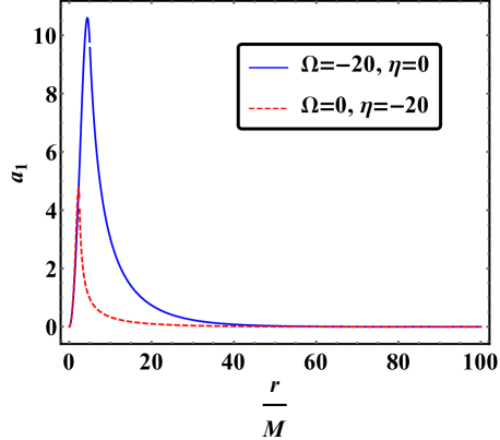
Figure 1: Unstable dipolar vector perturbation profile for a CD star. The solid blue line ($\eta=0,\Omega=-20$) corresponds to an instability rate $M\omega=0.094\rm i$ for a CD star compactness $M/R=0.2$. The dashed red line ($\Omega=0,\eta=-20$) corresponds to a rate $M\,\omega=0.071\,{\rm i}$ for a CD star compactness $M/R=0.4$.

We have solved numerically Eq. (15), for CD and Poly stars, as an eigenvalue problem for the frequencies $\omega$. In both cases, we have used direct integration to search for instabilities Macedo et al. (2016); GRI , looking for unstable solutions with purely imaginary frequency $\omega_{I}>0$, and imposing regularity at the center of the star and at infinity. Further details on the integration method are given in Appendix B.

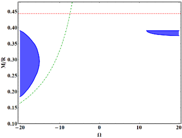
Figure 2: The shaded region represents CD (left) and Poly (right) star configurations with different values of $\Omega$ and $M/R$, which are unstable under axial perturbations in HN gravity with $\eta=0$. The green dot-dashed curve is the Newtonian solution for a CD star, Eq. (18). The dashed red line corresponds to the Buchdal limit on the compactness of a CD star ($M/R<4/9\approx 0.444$).

We found that unstable modes are present for some configurations, the properties of which are summarized in Figs. 1 and 2. Figure 1 shows the radial profile of dipolar ($l=1$) unstable modes for a CD star with compactness $M/R=0.2$ and couplings constants $(\Omega,\eta)=(-20,0)$ and for a CD star with compactness $M/R=0.4$ and coupling constants $(\Omega,\eta)=(0,-20)$.

When $\Omega,\eta>0$, we find unstable solutions as well. For each choice of $\eta$ and $\Omega$ we find a sequence of characteristic frequencies corresponding to unstable solutions with nodes.

In Fig. 2 we show the stability diagram for different values of the coupling constant $\Omega$, assuming $\eta=0$, obtained by considering dipolar axial perturbations of stellar configurations with different values of the compactness $M/R$. The left panel refers to CD stars, while the right panel refers to Poly stars. The shaded region corresponds to configurations which are unstable under axial perturbations. Strictly speaking, these regions correspond to instability to dipolar ($l=1$) perturbations, but we find strong evidence that the configurations unstable to $l>1$ axial perturbations are also unstable to dipolar ones. The dotted horizontal line represents the Buchdal limit $\frac{M}{R}<\frac{4}{9}$, which we verified to be satisfied in HN theory, while the dot-dashed curve corresponds to the Newtonian configurations for CD stars (see discussion below). Note that, as discussed above, for negative couplings $\Omega,\,\eta$, even Newtonian stars can become unstable. We find that unstable configurations also exists in the case of $\eta\neq 0$.

The separation between the stable and unstable regions, i.e. the boundaries of the shaded regions in Fig. -2, correspond to zero-mode solutions, i.e., static regular solutions with nonvanishing vector field. In order to improve our understanding of this boundary, we shall now consider zero-mode solutions in the Newtonian limit (i.e., $\frac{M}{R}\ll 1$) for a CD star. In this limit Eq. (15) reduces to

$$a_{l}^{\prime\prime}-\left(\frac{l(l+1)}{r^{2}}+\mu^{2}\right)a_{l}=0\,,$$ (17)

where $\mu^{2}=2\pi\rho(2\Omega+\eta)$ is the effective mass of the vector inside the star. Imposing regularity at the origin, the general solution of Eq. (17) inside the star is (modulo an arbitrary multiplicative constant) $a_{l}=\sqrt{r}J_{l+1/2}(-i\mu r)$, with $J_{\nu}$ Bessel function. Outside the star $\rho=0$ and imposing regularity at infinity Eq. (17) gives $a_{l}\propto r^{-l}$. Matching the interior and the exterior solution at the radius of the star $r=R$ we find that a regular solution exists only for $I_{l-1/2}(-i\mu R)=0$, where $I_{\nu}$ is the modified Bessel function, i.e., for $\mu R=i\pi$, which corresponds to

$$-3M\left(\eta+2\Omega\right)=2\pi^{2}R\,.$$ (18)

When $\eta=0$, this equation admits a nontrivial solution for negative values of $\Omega$. Thus, for $\eta=0$, $\Omega<0$ we expect the presence of unstable solutions.

The Newtonian prediction (18) is shown in Fig. 2 (green dot-dashed curve). We note that this line is close to the boundary of the unstable region, and it is closer for smaller values of the compactness, as expected. At fixed negative coupling constant $\Omega$, as the compactness increases to large values, the quantity $\rho-3P$ decreases. For Poly stars, at $M/R\sim 0.27$ it becomes negative. The effective squared mass of the vector (16) is then positive, and the star is stable. Thus, all the main features of Fig. 2 can be understood in simple terms. For the same reasons, unstable solutions lying on the right side of the plot (positive coupling constants) exist for very large values of the compactness, when the effective mass squared is again negative.

It is worth noting that our results resemble those of scalar-tensor theories (compare our Fig. 2 with Fig. 1 of Ref. Pani et al. (2011)). The root of the mechanism is the same: a tachyonic instability that is either triggered by a “wrong” sign of the coupling constants or by the wrong sign of the trace of the stress-energy tensor. Despite these similarities, we are here discussing the dipolar axial sector excitations of the vector field, which have a very different behavior from those of the scalar field. The end state of this instability is unknown to us.

Including backreaction on Einstein’s equations, the axial perturbations give a contribution to the $(\theta,\theta)$ component of Einstein’s equations, which can be considered as an effective stress-energy tensor. This suggests that the star will be made to rotate as a result of such instability. Another outcome is possible: that the star exits the instability window through mass shedding. The fate of stars on the unstable branch remains an open issue.

III.2 Spontaneous and induced vectorization in the polar sector

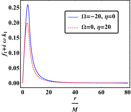
Figure 3: Unstable dipolar vector perturbation profile for a constant density star with compactness $M/R=0.2$. The solid blue line ($\eta=0,\Omega=-20$) corresponds to an instability rate $M\omega=0.103\rm i$. The dashed red line ($\Omega=0,\eta=20$) corresponds to a rate $M\,\omega=0.0989\rm i$.

Since we are interested in static and spherically symmetric solutions of the full non linear field equations in HN gravity, we shall now study linear vector field perturbations with polar parity in this theory.

Dynamical case. To begin with, let us consider monopolar ($l=0$) perturbations. In the exterior of the star, we find that the $l=0$ polar perturbation equations reduce to those of GR, i.e.

$$(\mathrm{i}\omega h_{0}+f_{0}^{\prime})\left(rFG^{\prime}+4FG-rGF^{\prime}\right)$$

$$+2rGF\left(\mathrm{i}\omega h_{0}+f_{0}^{\prime}\right)^{\prime}=0\,,$$

$$\omega\left(\mathrm{i}\omega h_{0}+f_{0}^{\prime}\right)=0\,.$$ (19)

Since the radial electric field $E_{r}$ is proportional to $\mathrm{i}\omega h_{0}+f_{0}^{\prime}$, when $\omega\neq 0$ the second of Eqs. (19) implies that $E_{r}=0$, and thus the wave is pure gauge: there are no spherically symmetric electromagnetic waves with radial electric fields in the exterior of the star, in HN gravity as in GR. Then, since the solution inside the star has to match the exterior solution, $E_{r}$ is pure gauge in the entire spacetime. In other words, there is no dynamical linear instability for spherically symmetric modes.

Let us now consider the polar perturbations with the $l\geq 1$ case. By replacing the expansion (14) in the $r$ component of Eq. (13) we find:

$$h_{l}=\frac{-l(l+1)Fk_{l}^{\prime}+\mathrm{i}r^{2}\omega f_{l}^{\prime}}{F\left(2\pi r^{2}((6\Omega+\eta)p-(\eta+2\Omega)\rho)-l(l+1)\right)+r^{2}\omega^{2}}.$$ (20)

Replacing Eq. (20) in the $t$ and $\theta$ components of Eq. (13) we obtain a system of coupled ordinary differential equations (ODEs) in $f_{l}$ and $k_{l}$, that is shown in Appendix A, Eqs. (A) and (A).

The perturbation equations have simpler expressions in the exterior of the star. Indeed, as $\rho=p=0$ Eqs. (A) and (A) can be cast as a single “master equation” in terms of the quantity

$$\psi=f_{l}+\mathrm{i}\omega k_{l}\,,$$ (21)

which is:

$$\frac{\left(l^{2}+l\right)\psi}{2Mr-r^{2}}+\frac{l(l+1)(2M-r)\psi^{\prime\prime}}{l(l+1)(2M-r)+r^{3}w^{2}}$$

$$+\frac{2l(l+1)\left(l(l+1)(r-2M)^{2}-Mr^{3}w^{2}\right)\psi^{\prime}}{r\left(l(l+1)(2M-r)+r^{3}w^{2}\right)^{2}}=0\,.$$ (22)

Solving the Cauchy problem given by Eqs. (A) and (A), with appropriate initial conditions (as discussed in Appendix B) and matching at the boundary of the star with Eq. (III.2), we find unstable configurations for CD stars. In Fig. 3, for instance, we show the radial profile of an unstable mode with $l=1$ for a constant density star of compactness $M/R=0.2$, for $\Omega=-20,\eta=0$ or $\eta=20,\Omega=0$. As in the case of axial perturbations, we can construct the instability diagram in the space ($\Omega,M/R$). The static zero-mode solutions in the Newtonian limit $M/R\ll 1$ yields

$$3M\left(\eta-2\Omega\right)=2\pi^{2}R\,.$$ (23)

In Fig. 4 we show the instability region (shaded region) in the ($\Omega,M/R$) plan, for $\eta=0$ and negative values of the coupling constant $\Omega$. The horizontal dotted line represents the Buchdal limit, and the dot-dashed curve represents the Newtonian zero-mode solutions corresponding to Eq. (23).

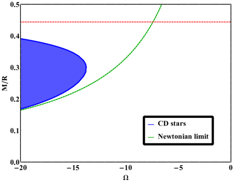
Figure 4: Instability diagram for CD stars, for polar perturbations with $l=1$. The shaded region represents solutions which are unstable under polar perturbations in HN gravity with $\eta=0$. The green dot-dashed curve describes zero-frequency modes in the Newtonian regime, Eq. (23). The dashed red line corresponds to the Buchdal limit ($M/R<4/9\approx 0.444$).

An interesting feature of these results is that the contribution of the coupling $\eta$ to the effective mass squared has opposite sign from that of axial perturbations: large negative $\eta$ make Newtonian stars unstable against axial perturbations, and large positive $\eta$ turn Newtonian stars unstable against polar perturbations.

Static case. We showed that spherically symmetric polar modes have no interesting dynamics. However, there is still room for the existence of nontrivial static ($\omega=0$) solutions. Replacing the expansion (14) in the field equations (13) we find:

$$h_{0}=0\,,$$ (24)

and,

$$\big{[} -f_{0}^{\prime}\left(2r\left(m^{\prime}-2\right)+r(r-2m)\nu^{\prime}+6m\right)+2r(r-2m)f_{0}^{\prime\prime}$$

$$+4\pi r^{2}(2\Omega(3p-\rho)+\eta(3p+\rho))f_{0}\big{]}\frac{e^{-\nu}}{2r^{2}}=0\,.$$ (25)

Solving Eq.(25) we find a class of linear static vector field solutions, for both the CD and the Poly star configurations. Equation (25) also implies an analytical relation between the compactness and the coupling constant, in the Newtonian regime for a CD star. Indeed, since $h_{0}=0$, we can assume the following form for the vector field:

$$X_{\mu}=(f_{0}(r)/r,0,0,0)\,.$$ (26)

In the limit $M/R\ll 1$, for a CD star Eq. (25) reduces to

$$f_{0}^{\prime\prime}-\mu^{2}f_{0}=0\,,$$ (27)

where $\mu^{2}=2\pi\rho(2\Omega-\eta)$ is the effective mass of the vector inside the star. Imposing regularity at the origin we find $f_{0}=e^{\mu r}-e^{-\mu r}$ inside the star, and imposing regularity at infinity we find $f_{0}=const.$ in the exterior. By matching the interior and exterior solutions at the radius of the star we find

$$6M(\eta-2\Omega)=\pi^{2}R\,.$$ (28)

The static solutions are summarized in Fig.5. These solutions might be said to be induced, rather than arising spontaneously as the end product of an instability: they arise as the end product of (perhaps special) initial conditions. Such vectorized solutions have no parallel in scalar-tensor theory and do not exist in the axial sector of HN gravity itself. Note again that $\eta$ contributes with the opposite sign, relative to axial perturbations in Eq. (17).

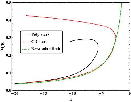
Figure 5: Linear static vector field solutions for a NS background (solid black line) and for a CD star (dot-dashed red line) for $\eta=0$. The dashed green line corresponds to the Newtonian analytic solution for the polar sector in the CD star background.

From these solutions we can conclude that in GR, a vector field coupled with the curvature of the spacetime can have a nontrivial profile around compact stars. Moreover, this result suggests that vectorized stars can appear even in full nonlinear HN gravity.

We should mention that, generically, the vector $X_{\mu}$ will tend to grow all its components. Thus, with the exception of a measure-zero set of initial conditions, finding only a nonzero timecomponent is impossible. In other words, the spherically symmetric state that occurs at linear (and nonlinear, as we show below) level is not generic and should always be accompanied by the linear instability of the nonsymmetric modes. However, from a purely mathematical level the distinction between induced and spontaneous processes can be made and we have adopted such nomenclature here.

IV Static, vectorized neutron stars in the HN theory

IV.1 Formalism

We shall now determine full nonlinear, stationary and spherically symmetric NS configurations in HN theory, solutions of Eqs. (2) and (3). In other words, we show that the induced vectorized solutions, found above at a linear level, do indeed exist at full nonlinear level. Hereafter, we assume $\eta=0$. For convenience, we rewrite the line element of Eq. (7) defining $F=e^{\nu(r)}$ and $G=1-\frac{2m(r)}{r}$. A spherically symmetric vector field can only have nonvanishing $t$- and $r$- components. Moreover, the $r$ component of the vector field equation reduces to

$$\frac{X_{r}}{4r^{3}}\Big{[}\Omega(r-2m)(-2m^{\prime}(r\nu^{\prime}+4)+(4r-6m)\nu^{\prime})$$

$$+2r(r-2m)\nu^{\prime\prime}+r(r-2m)\nu^{\prime 2}\Big{]}=0$$ (29)

which implies $X_{r}\equiv 0$. Therefore, all the space components of the vector field identically vanish:

$$X_{\mu}=\left\{X(r),0,0,0\right\}\,.$$ (30)

The structure equations for the star are given by the $(t,t)$, $(r,r)$ components of the Einstein equations (2), the vector field equation (3) and the conservation of the stress-energy tensor:

$$\nabla_{\nu}T^{\mu\nu}=0\,.$$ (31)

We note that Eq. (31) holds in HN gravity because the GR modifications do not affect the matter section of the action (1); therefore, as explicitly shown in Ref. Will (1993), the four-divergence of the stress-energy tensor vanishes in this theory, as in GR. We thus obtain a system of four ODEs in the variables

$$\left\{m(r),\nu(r),p(r),X(r)\right\}\,.$$ (32)

These modified Tolman-Oppenheimer-Volkoff (TOV) equations are shown explicitly in Appendix C, Eq. (C); their expansion near the center of the star is shown in Appendix D.

We numerically solve the modified TOV equations, assuming the polytropic EOS introduced in Eq. (11). At the surface of the star (where the pressure vanishes) we evaluate the components of the spacetime metric, of the vector field and of its first derivative. Then, we numerically integrate the equations in the exterior, which correspond to the modified TOV equations with $\rho=p=0$, from the stellar surface to infinity. With this procedure, we have a unique solution of the modified TOV equations for any choice of the quantities

$$\left\{p_{c},X_{c},\Omega\right\}\,,$$ (33)

i.e. for any choice of the pressure and of the (time component of the) vector field at the center of the star, and for any value of the coupling constant $\Omega$. At infinity, the vector field has the form

$$X_{0}(r\gg R)=X_{\rm\infty}+\frac{\alpha}{r}\,,$$ (34)

where $\alpha$ is a constant which can be considered as a sort of vector charge (although it is not a Noether charge, as in the case of the scalar charge in scalar-tensor theories Esposito-Farese (2004)), and $X_{\rm\infty}$ is the asymptotic value of (the time component of) the vector field.

We search for solutions of the modified TOV equations with a nontrivial vector field configuration, and with the same asymptotic behavior as GR solutions, i.e., $X_{\rm\infty}=0$. Is it worth noting that the mass function does not remain constant in the exterior of the star, due to the energy contribution of the nontrivial vector field. The gravitational mass that a far away observer can measure, i.e., the Arnowitt-Deser-Misner mass of the spacetime, is the asymptotic value of $M(r)$. This is the definition of gravitational mass that we are going to use in the rest of the paper.

The baryonic mass of the NS is defined as Misner et al. (1973)

$$\bar{m}=m_{b}\int d^{3}x\sqrt{-g}u^{0}n(r)\,,$$ (35)

where $u^{0}$ is the time component of the four-velocity and $n(r)$ is the number density of baryons, which is related to the pressure by

$$p(r)=Kn_{0}m_{b}\left(\frac{n(r)}{n_{0}}\right)^{\Gamma}\,.$$ (36)

For each vectorized solution, we can evaluate the normalized binding energy of the stars defined as,

$$\frac{E_{b}}{M}=\frac{\bar{m}}{M}-1\,.$$ (37)

In order to have a bound object, we need $E_{b}$ to be positive. Moreover, the dependence of the gravitational mass on the central density often conveys information on the stability of the configuration. Indeed, in GR a necessary condition for radial stability of a stellar configuration is $dM/d\rho_{c}<0$, or equivalently $dM/dR>0$ Friedman et al. (1988); Shapiro and Teukolsky (1983). The condition for stability in generalized theories depends on the number of extra fields, and becomes more complicated Brito et al. (2016).

IV.2 Vectorized stars

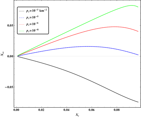
Figure 6: Time component of the vector field at infinity, as a function of its value at the center of the star, for $\Omega=-5$ and for different values of the central pressure. From top to bottom, $p_{c}=10^{-8},10^{-7},10^{-6},10^{-5},10^{-4},10^{-3}\,{\rm Km}^{-2}$.

In Fig. 6 we show the results of the numerical integration of the modified TOV equations in the case of $\Omega=-5$. In the figure the asymptotic value of the vector field, $X_{\rm\infty}$, is shown as a function of the vector field at the center, $X_{c}$. Each curve corresponds to a different value of the central pressure $p_{c}$. The “physical” solutions, i.e., those with the same asymptotic behavior as the GR solutions, correspond to the intersections of the curves with the $X_{\rm\infty}=0$ axis. We see that all curves intersect the $X_{\rm\infty}=0$ axis at the origin (corresponding to the GR solution), but some of them also have a second intersection, which corresponds to the vectorized solutions.

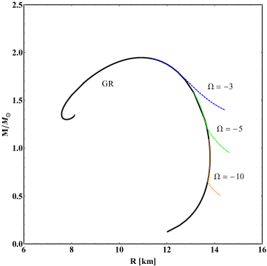
Figure 7: Mass-radius configurations for different coupling constants. The longest line (black) represents the solution for NSs in GR given the EOS in Eq. (11), while the other branches correspond to vectorized solutions.

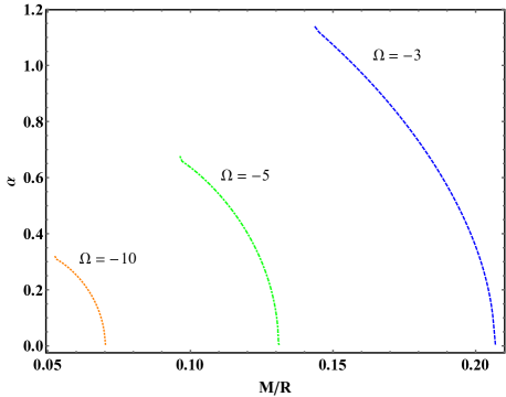
Figure 8: Vector field charge as a function of the compactness, for different stellar configurations. All the stars carrying a zero charge ($\alpha=0$) are always a solution of the theory, although they are not explicitly shown in the figure. In fact, in the range in which there are stars with a nonzero charge, the solutions are always two, as it was clear from Fig.6.

We computed the vectorized solutions for a wide range of values of the central pressure and of the coupling constant $\Omega$. The masses and the radii of these configurations are shown in Fig. 7; the corresponding values of the vector charge $\alpha$ (see Eq. (34)) is shown in Fig. 8 as a function of the compactness. We can see that comparing different compact star configurations (for a given value of the coupling $\Omega$), as the compactness decreases there is a smooth transition between GR stars and vectorized solutions. Then, below a threshold value of the compactness, the vectorized solution does not exist anymore. As discussed in Appendix D, this behavior is due to the fact that, when the compactness reaches the threshold value, the modified TOV equation are not well behaved near the center of the star, since they become degenerate. Below the threshold value, the weak energy condition is violated, leading to an unphysical object. For positive values of $\Omega$, our linearized results (see Sec. III) suggest that there is more than one solution corresponding to every value of the central pressure, with different numbers of nodes in the profile of $X_{0}(r)$.

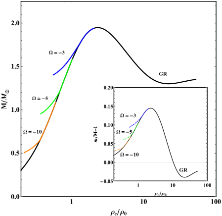
Figure 9: Gravitational mass as a function of the (normalized) central baryonic density. This shows again that the solutions for $\Omega<0$ are stable solutions of the theory, since they are associated with $dM/d\rho_{c}<0$. (Inset) The normalized binding energy as a function of the central energy density.

We did not perform a dynamical stability analysis of such vectorized solutions. However, important information is conveyed by the dependence of the total (normalized) gravitational mass on the central energy density ($\rho_{c}=m_{b}n(0)$). This function is shown in Fig. 9. In GR, a criterium for stability is that $dM/d\rho_{c}<0$. Such criterium holds only approximately in modified theories Harada (1998); Brito et al. (2016). We will use this as merely indicative, as more sophisticated analysis tools include a dynamical evolution or the analysis done in Ref. Brito et al. (2016). With such criterium, all the vectorized solutions associated with a negative coupling constant are stable: they are in the stable branch of the $dM/d\rho_{c}$ curve. Moreover, in the inset of Fig. 9 we can see how the solutions in vector-tensor theory are associated with larger binding energy than in GR, indicating that they are the preferred configuration. For positive couplings, however, the behavior is the opposite.

Finally, we note that the instability of solutions in the positive $\Omega$ semiplane is consistent with previous results in scalar-tensor gravity Mendes and Ortiz (2016). Thus, none of the solutions associated with a positive coupling constant are stable and most likely do not play any astrophysical role.

Somewhat surprisingly, our results show that the changes in the NS structure with respect to the GR are smaller for larger values of the coupling constants. This finding is consistent with previous reported results in a related theory Ramazanoğlu (2017). In fact, it is apparent from Fig. 8 that the charge (and so the field) inside vectorized stars is larger for smaller (absolute) values of the compactness. This is probably due to the role of the coupling constant $\Omega$ in the modified TOV system. In fact, it resembles the role of a mass for the scalar field in scalar-tensor gravity: the larger the scalar mass, the smaller are the modifications from GR. Taking into account this, from the mass-radius plot one can quantify the range of values of $\Omega$ that allow vectorized stars to exist,

$$\Omega\approx[-12,-2]\,.$$ (38)

Finally, let us stress that there is no linear instability of spherically symmetric stars in GR. Thus, there is no linear mechanism to drive a GR star to these new vectorized states that we just described. Such vectorized spherical stars must therefore arise out of nonlinear effects (such as selected initial conditions).

V Discussion

We have shown that very simple extensions of the Einstein-Maxwell theory allow for nontrivial phenomena to exist. Once curvature couplings are allowed, general relativistic stars are allowed but generically unstable. We are unable at this point to follow the evolution of such instability or even to understand its end state, since it drives a nonspherically symmetric mode. The end state could be a star with a nontrivial vector field, but it could also simply be a GR solution away from the instability region.

We find interesting novel spherically symmetric star configurations in this theory. They do not seem to arise out of any “spontaneous-vectorization” mechanism but are rather induced by initial conditions. These stars carry a nonzero electric charge and give rise to dipolar electromagnetic radiation when accelerated. The calculation of such fluxes and its use in astrophysical observations to constrain the coupling constants is an interesting open problem.

Appendix A Equations for polar perturbations

The perturbation equations with polar parity are

$$\frac{Gf_{l}^{\prime\prime}(1-\frac{r^{2}\omega^{2}}{F(2\pi r^{2}((6\Omega+\eta)p-(\eta+2\Omega)\epsilon)-l(l+1))+r^{2}\omega^{2}})}{F}+\frac{il(l+1)\omega Gk_{l}^{\prime\prime}}{F(l(l+1)+2\pi r^{2}((-\eta-6\Omega)p-(-\eta-2\Omega)\epsilon))-r^{2}\omega^{2}}$$

$$-\frac{f_{l}(l(l+1)+2\pi r^{2}(3(-\eta-2\Omega)p+(-\eta+2\Omega)\epsilon))}{r^{2}F}-\frac{il(l+1)\omega k_{l}}{r^{2}F}$$

$$+\frac{il(l+1)\omega k_{l}^{\prime}}{2rF(F(2\pi r^{2}((6\Omega+\eta)p+(-\eta-2\Omega)\epsilon)-l(l+1))+r^{2}\omega^{2})^{2}}(rF(-GF^{\prime}(l(l+1)$$

$$+2\pi r^{2}((-\eta-6\Omega)p-(-\eta-2\Omega)\epsilon))-r^{2}\omega^{2}G^{\prime})+r^{3}(-\omega^{2})GF^{\prime}+F^{2}(rG^{\prime}(l(l+1)+2\pi r^{2}((-\eta-6\Omega)p$$

$$-(-\eta-2\Omega)\epsilon))+4G(l(l+1)+\pi r^{3}((6\Omega+\eta)p^{\prime}+(-\eta-2\Omega)\epsilon^{\prime}))))$$

$$-\frac{f_{l}^{\prime}}{2rF(F(2\pi r^{2}((6\Omega+\eta)p+(-\eta-2\Omega)\epsilon)-l(l+1))+r^{2}\omega^{2})^{2}}(rF(G(l^{2}(l+1)^{2}F^{\prime}$$

$$+4\pi r^{2}((-\eta-6\Omega)p(F^{\prime}(l(l+1)-2\pi r^{2}(-\eta-2\Omega)\epsilon)+2r\omega^{2})-(-\eta-2\Omega)\epsilon(l(l+1)F^{\prime}+2r\omega^{2})$$

$$+\pi r^{2}(-\eta-6\Omega)^{2}p^{2}F^{\prime}+\pi r^{2}(-\eta-2\Omega)^{2}\epsilon^{2}F^{\prime}+r^{2}\omega^{2}((-\eta-6\Omega)p^{\prime}-(-\eta-2\Omega)\epsilon^{\prime})))+r^{2}\omega^{2}G^{\prime}(l(l+1)$$

$$+2\pi r^{2}((-\eta-6\Omega)p-(-\eta-2\Omega)\epsilon)))+r^{3}\omega^{2}GF^{\prime}(l(l+1)$$

$$+2\pi r^{2}((-\eta-6\Omega)p-(-\eta-2\Omega)\epsilon))-F^{2}(rG^{\prime}+4G)(l(l+1)+2\pi r^{2}((-\eta-6\Omega)p-(-\eta-2\Omega)\epsilon))^{2})=0\,,$$ (39)

$$+\frac{i\omega Gf_{l}^{\prime\prime}}{F(2\pi r^{2}((6\Omega+\eta)p-(\eta+2\Omega)\epsilon)-l(l+1))+r^{2}\omega^{2}}+\frac{i\omega f_{l}}{r^{2}F}$$

$$-\frac{Gk_{l}^{\prime\prime}(2\pi F((6\Omega+\eta)p+(-\eta-2\Omega)\epsilon)+\omega^{2})}{F(2\pi r^{2}((6\Omega+\eta)p+(-\eta-2\Omega)\epsilon)-l(l+1))+r^{2}\omega^{2}}+\frac{k_{l}(2\pi F((-\eta-6\Omega)p-(-\eta-2\Omega)\epsilon)-\omega^{2})}{r^{2}F}$$

$$+\frac{i\omega f_{l}^{\prime}}{2rF(F(2\pi r^{2}((6\Omega+\eta)p+(-\eta-2\Omega)\epsilon)-l(l+1))+r^{2}\omega^{2})^{2}}(rF(GF^{\prime}(l(l+1)$$

$$+2\pi r^{2}((-\eta-6\Omega)p-(-\eta-2\Omega)\epsilon))+r^{2}\omega^{2}G^{\prime})+r^{3}\omega^{2}GF^{\prime}+F^{2}(4G(\pi r^{3}((-\eta-6\Omega)p^{\prime}$$

$$-(-\eta-2\Omega)\epsilon^{\prime})-l(l+1))-rG^{\prime}(l(l+1)+2\pi r^{2}((-\eta-6\Omega)p-(-\eta-2\Omega)\epsilon))))$$

$$-\frac{k_{l}^{\prime}}{2rF(F(2\pi r^{2}((6\Omega+\eta)p+(-\eta-2\Omega)\epsilon)-l(l+1))+r^{2}\omega^{2})^{2}}(r\omega^{2}F(GF^{\prime}(l(l+1)$$

$$+4\pi r^{2}((6\Omega+\eta)p+(-\eta-2\Omega)\epsilon))+r^{2}\omega^{2}G^{\prime})-F^{2}(-2\pi rGF^{\prime}((-\eta-6\Omega)p$$

$$-(-\eta-2\Omega)\epsilon)(l(l+1)+2\pi r^{2}((-\eta-6\Omega)p-(-\eta-2\Omega)\epsilon))+r\omega^{2}G^{\prime}(l(l+1)+4\pi r^{2}((-\eta-6\Omega)p$$

$$-(-\eta-2\Omega)\epsilon))+4l(l+1)\omega^{2}G)+r^{3}\omega^{4}GF^{\prime}+2\pi F^{3}(rG^{\prime}((-\eta-6\Omega)p-(-\eta-2\Omega)\epsilon)(l(l+1)$$

$$+2\pi r^{2}((-\eta-6\Omega)p-(-\eta-2\Omega)\epsilon))+2l(l+1)G(r(-\eta-6\Omega)p^{\prime}+2(-\eta-6\Omega)p$$

$$-r(-\eta-2\Omega)\epsilon^{\prime}-2(-\eta-2\Omega)\epsilon)))=0\,.$$ (40)

Appendix B Numerical integration of the perturbation equations

We here discuss the numerical integration of perturbation equations of static, spherically symmetric stars in HN gravity. In order to enforce a regular behavior near the center of the star, we perform an asymptotic expansion of the axial perturbation equation (15), by expanding the perturbation function as

$$a_{l}=\sum_{i=0}^{N}a_{l}^{i}r^{i}\,.$$ (41)

We truncate the expansion at $N=4$ because we found that further coefficient does not affect significantly the results. Thus, we find the values of the coefficients $a_{l}^{i>0}$ in terms of $a_{l}^{0}$ (which can be set to an arbitrary value). In terms of these coefficients we can compute $a_{l}(r_{0})$ and $a_{l,r}(r_{0})$ at $r_{0}\ll R$. We then numerically integrate Eq. (15) from $r_{0}$ to the surface of the star $r=R$ and, imposing regularity of the perturbations, from the surface to $r\gg R$.

Unstable modes have frequency $\omega=\omega_{R}+\rm{i}\omega_{I}$, with $\omega_{I}>0$. Since we look for the onset of the instability, we look for solutions with purely imaginary frequency, i.e., $\omega_{R}=0$, by matching the solution far away from the star with

$$a_{l}(r)\approx e^{\omega_{\text{\rm{I}}}r}c_{1}+e^{-\omega_{\text{\rm{I}}}r}c_{2}\,,$$ (42)

where $c_{1}$ and $c_{2}$ are two constants of integration. Finally, since we require an asymptotically flat spacetime, we impose $c_{1}=0$. We thus find a perturbation which grows in time and regular at spatial infinity, behaving asymptotically as

$$a_{l}(t,r)=c_{2}e^{-\omega_{\text{I}}r}e^{\omega_{\text{I}}t}\,.$$ (43)

In order to solve the perturbation equations with polar parity (A) and (A), we follow the same approach. The only difference is that, for each value of the harmonic index $l$, we have two perturbation functions, $f_{l}(r)$ and $k_{l}(r)$.

Appendix C Modified TOV equations

In the following, we show the full nonlinear system of equations that describes static, nonrotating stars in HN gravity:

$$\frac{e^{-\nu}}{2r^{2}}\big{[}-4e^{2\nu}(4\pi r^{2}\rho-m^{\prime})-4r^{2}X^{\prime 2}+-e^{\nu}\Omega X^{2}(4m^{\prime}(r\nu^{\prime}+1)+4(3m-2r)\nu^{\prime}+r(r-2m)(\nu^{\prime 2}-4\nu^{\prime\prime}))$$

$$-e^{\nu}(4\Omega X(r(r-2m)X^{\prime\prime}-X^{\prime}(rm^{\prime}+2r(r-2m)\nu^{\prime}+3m-2r))+2r(2\Omega-1)(r-2m)X^{\prime 2})\big{]}=0\,,$$

$$\frac{e^{-\nu}}{2r^{2}(r-2m)}\big{[}2m(-2r^{2}(4e^{\nu}-1)X^{\prime 2}-2e^{\nu}(r\nu^{\prime}+1)-2r\Omega X(r\nu^{\prime}+4)X^{\prime}+\Omega X^{2}(r\nu^{\prime}(r\nu^{\prime}+2)-2))$$

$$+16rm^{2}e^{\nu}X^{\prime 2}+r^{2}(-16\pi rpe^{\nu}+2\Omega X(r\nu^{\prime}+4)X^{\prime}+2e^{\nu}(\nu^{\prime}+2rX^{\prime 2})-2rX^{\prime 2}-\Omega X^{2}\nu^{\prime}(r\nu^{\prime}+2))\big{]}=0\,,$$

$$\frac{e^{-\nu}}{4r^{2}}\big{[}-2X^{\prime}(2r(m^{\prime}-2)+r(r-2m)\nu^{\prime}+6m)$$

$$+\Omega X(-2m^{\prime}(r\nu^{\prime}+4)+2(2r-3m)\nu^{\prime}+r(r-2m)(2\nu^{\prime\prime}+\nu^{\prime 2}))+4r(r-2m)X^{\prime\prime}\big{]}=0\,,$$

$$\frac{(r-2m)(2p^{\prime}+(p+\rho)\nu^{\prime})}{2r}=0\,,$$ (44)

This system is invariant if under the transformation

$$\{\nu(r)\rightarrow\nu_{0}+\tilde{\nu}(r),\,X\rightarrow e^{\frac{\nu_{0}}{2}}\tilde{X}\}\,,$$ (45)

where $\nu_{0}$ is an arbitrary constant.

Appendix D Expansion at the center of the modified TOV equations

The asymptotic expansion near the center of the star of the modified TOV equations (C) is:

$$\rho =\rho_{c}+\rho_{1}r+\frac{\rho_{2}}{2}r^{2}\,,$$

$$p(r) =p_{c}+p_{1}r+\frac{p_{2}}{2}r^{2}\,,$$

$$\nu(r) =\nu_{c}+\nu_{1}r+\frac{\nu_{2}}{2}r^{2}\,,$$ (46)

$$X(r) ={X}_{c}+{X}_{1}r+{X}_{2}\frac{r^{2}}{2}\,,$$

$$m(r) =m_{3}r^{3}\,.$$

Performing the transformation (45), we solve the modified TOV equations for $\tilde{\nu}=\nu-\nu_{c}$ and $\tilde{X}$. Comparing order by order, the nonvanishing coefficients of the expansion (46) are

$$m_{3} =\frac{4\pi\left(3p_{c}\tilde{X}_{c}^{2}\Omega(\Omega+2)+\rho_{c}\left(\tilde{X}_{c}^{2}\Omega(2\Omega+1)-1\right)\right)}{9\tilde{X}_{c}^{2}\Omega^{2}\left(\tilde{X}_{c}^{2}(\Omega-1)+1\right)-3}\,,$$

$$\tilde{\nu}_{2} =\frac{8\pi\Big{(}3p_{c}\left(\tilde{X}_{c}^{2}\Omega(2\Omega+1)-1\right)}{9\tilde{X}_{c}^{2}\Omega^{2}\left(\tilde{X}_{c}^{2}(\Omega-1)+1\right)-3}$$

$$+\frac{8\pi\rho_{c}\left(\tilde{X}_{c}^{2}\Omega(4\Omega-1)-1\right)\Big{)}}{9\tilde{X}_{c}^{2}\Omega^{2}\left(\tilde{X}_{c}^{2}(\Omega-1)+1\right)-3}\,,$$

$$\tilde{X}_{0,2} =\frac{4\pi\tilde{X}_{c}\Omega\left(3\tilde{X}_{c}^{2}\Omega(3p_{c}+\rho_{c})+3p_{c}-\rho_{c}\right)}{9\tilde{X}_{c}^{2}\Omega^{2}\left(\tilde{X}_{c}^{2}(\Omega-1)+1\right)-3}\,,\,$$

$$p_{2} =-\frac{4\pi(p_{c}+\rho_{c})\Big{(}3p_{c}\left(\tilde{X}_{c}^{2}\Omega(2\Omega+1)-1\right)}{9\tilde{X}_{c}^{2}\Omega^{2}\left(\tilde{X}_{c}^{2}(\Omega-1)+1\right)-3}$$

$$-\frac{4\pi(p_{c}+\rho_{c})\rho_{c}\left(\tilde{X}_{c}^{2}\Omega(4\Omega-1)-1\right)\Big{)}}{9\tilde{X}_{c}^{2}\Omega^{2}\left(\tilde{X}_{c}^{2}(\Omega-1)+1\right)-3}\,.$$ (47)

In the limit $\Omega=0$ these coefficients reduce to those of the TOV equations in GR. Moreover, we note that as

$$9\tilde{X}_{c}^{2}\Omega^{2}\left(\tilde{X}_{c}^{2}(\Omega-1)+1\right)-3=0$$ (48)

all the coefficients defined in (D) diverge. Thus, when Eq. (48) admits solution $r=\bar{r}$ inside the star, i.e. $0\leq\bar{r}\leq R$, then the modified TOV equations do not allow for a regular vectorized solution. Since, as the compactness of the star decreases, the root $\bar{r}$ becomes smaller, this is the reason for the existence of a threshold compactness under which the vectorized solution disappears (see e.g. Fig. 8).

References

- Lange et al. (2001) C. Lange, F. Camilo, N. Wex, M. Kramer, D. C. Backer, A. G. Lyne, and O. Doroshenko, Mon. Not. Roy. Astron. Soc. 326, 274 (2001), arXiv:astro-ph/0102309 [astro-ph] .
- Antoniadis et al. (2013) J. Antoniadis et al., Science 340, 6131 (2013), arXiv:1304.6875 [astro-ph.HE] .
- Abbott et al. (2017) B. Abbott et al. (Virgo, LIGO Scientific), Phys. Rev. Lett. 119, 161101 (2017), arXiv:1710.05832 [gr-qc] .
- Lightman et al. (1975) A. P. Lightman, W. H. Press, R. H. Price, and S. A. Teukolsky, Problem Book in Relativity and Gravitation, by A. Lightman and R.H. Price. Princeton: Princeton University Press, 1975. (1975).
- Hellings and Nordtvedt (1973) R. W. Hellings and K. Nordtvedt, Phys. Rev. D7, 3593 (1973).
- Eidelman et al. (2004) S. Eidelman et al. (Particle Data Group), Phys. Lett. B592, 1 (2004).
- Pani et al. (2012) P. Pani, V. Cardoso, L. Gualtieri, E. Berti, and A. Ishibashi, Phys. Rev. Lett. 109, 131102 (2012), arXiv:1209.0465 [gr-qc] .
- Polchinski (2007) J. Polchinski, String theory. Vol. 1: An introduction to the bosonic string, Cambridge Monographs on Mathematical Physics (Cambridge University Press, 2007).
-
Essig et al. (2013)
R. Essig et al., in Proceedings, 2013 Community Summer Study on the Future of U.S. Particle
Physics: Snowmass on the Mississippi (CSS2013): Minneapolis, MN, USA, July
29-August 6, 2013 (http://www.slac.stanford.edu/econf/C1307292/docs/
IntensityFrontier/NewLight-17.pdf, 2013) arXiv:1311.0029 [hep-ph] . - Heisenberg (2014) L. Heisenberg, JCAP 1405, 015 (2014), arXiv:1402.7026 [hep-th] .
- Damour and Esposito-Farese (1993) T. Damour and G. Esposito-Farese, Phys. Rev. Lett. 70, 2220 (1993).
- Pani et al. (2011) P. Pani, V. Cardoso, E. Berti, J. Read, and M. Salgado, Phys. Rev. D83, 081501 (2011), arXiv:1012.1343 [gr-qc] .
- Will (1993) C. M. Will, Theory and experiment in gravitational physics (1993).
- Antoniadis et al. (2012) J. Antoniadis, M. H. van Kerkwijk, D. Koester, P. C. C. Freire, N. Wex, T. M. Tauris, M. Kramer, and C. G. Bassa, Mon. Not. Roy. Astron. Soc. 423, 3316 (2012), arXiv:1204.3948 [astro-ph.HE] .
- Berti et al. (2015) E. Berti et al., Class. Quant. Grav. 32, 243001 (2015), arXiv:1501.07274 [gr-qc] .
- Ramazanoglu and Pretorius (2016) F. M. Ramazanoglu and F. Pretorius, Phys. Rev. D93, 064005 (2016), arXiv:1601.07475 [gr-qc] .
- Ramazanoğlu (2017) F. M. Ramazanoğlu, Phys. Rev. D96, 064009 (2017), arXiv:1706.01056 [gr-qc] .
- Ramazanoğlu (2019) F. M. Ramazanoğlu, Phys. Rev. D99, 044003 (2019), arXiv:1901.00194 [gr-qc] .
- Shapiro and Teukolsky (1983) S. L. Shapiro and S. A. Teukolsky, Black holes, white dwarfs, and neutron stars: The physics of compact objects (1983).
- Lima et al. (2010) W. C. C. Lima, G. E. A. Matsas, and D. A. T. Vanzella, Phys. Rev. Lett. 105, 151102 (2010), arXiv:1009.1771 [gr-qc] .
- Macedo et al. (2016) C. F. B. Macedo, V. Cardoso, L. C. B. Crispino, and P. Pani, Phys. Rev. D93, 064053 (2016), arXiv:1603.02095 [gr-qc] .
-
(22)
Gravity at Técnico: GRIT:
https://centra.tecnico.ulisboa.pt/network/grit/files/ . - Esposito-Farese (2004) G. Esposito-Farese, Phi in the sky: The quest for cosmological scalar fields. Proceedings, Workshop, Porto, Portugal, July 8-10, 2004, AIP Conf. Proc. 736, 35 (2004), [,35(2004)], arXiv:gr-qc/0409081 [gr-qc] .
- Misner et al. (1973) C. W. Misner, K. S. Thorne, and J. A. Wheeler, Gravitation (W. H. Freeman, San Francisco, 1973).
- Friedman et al. (1988) J. L. Friedman, J. R. Ipser, and R. D. Sorkin, Astrophys. J. 325, 722 (1988).
- Brito et al. (2016) R. Brito, V. Cardoso, C. F. B. Macedo, H. Okawa, and C. Palenzuela, Phys. Rev. D93, 044045 (2016), arXiv:1512.00466 [astro-ph.SR] .
- Harada (1998) T. Harada, Phys. Rev. D57, 4802 (1998), arXiv:gr-qc/9801049 [gr-qc] .
- Mendes and Ortiz (2016) R. F. P. Mendes and N. Ortiz, Phys. Rev. D93, 124035 (2016), arXiv:1604.04175 [gr-qc] .