Magnetic island merger as a mechanism for inverse magnetic energy transfer

Abstract

Magnetic energy transfer from small to large scales due to successive magnetic island coalescence is investigated. A solvable analytical model is introduced and shown to correctly capture the evolution of the main quantities of interest, as borne out by numerical simulations. Magnetic reconnection is identified as the key mechanism enabling the inverse transfer, and setting its properties: magnetic energy decays as $\tilde{t}^{-1}$, where $\tilde{t}$ is time normalized to the (appropriately defined) reconnection timescale; and the correlation length of the field grows as $\tilde{t}^{1/2}$. The magnetic energy spectrum is self-similar, and evolves as $\propto\tilde{t}^{-3/2}k^{-2}$, where the $k$-dependence is imparted by the formation of thin current sheets.

Introduction.

The transfer of magnetic energy from small to large spatial scales is a poorly understood plasma process of fundamental relevance to a variety of space and astrophysical environments. It may, for example, play a critical role in the origin of large-scale galactic magnetic fields Kulsrud and Zweibel (2008), by enabling kinetic-scale seed fields (e.g., Weibel Weibel (1959) generated) to develop spatial coherence on larger, perhaps fluid, scales Gruzinov (2001). Ultimately, the questions are not only whether such an inverse cascade is possible, but also how rapid and efficient it is — i.e., can an inverse cascade deliver significant amounts of magnetic energy to scales where ambient turbulence may efficiently amplify it via turbulent dynamo processes?

Similarly motivated issues arise in the context of gamma-ray bursts (GRBs) where one wonders if Weibel-produced fields in the relativistic shock Medvedev and Loeb (1999) can survive long enough to explain the observed powerful synchrotron emission Gruzinov (2001). In the space-physics context, a frequently encountered question concerns the dynamic evolution of a complex, volume-filling “sea” of flux ropes or magnetic islands, e.g., in the solar wind and the outer heliosphere Manchester IV et al. ; Klimchuk et al. (2008); Khabarova et al. (2015); Drake et al. (2012).

Past theoretical work on inverse magnetic energy transfer has mainly developed along two directions: the study of decaying turbulence, where the time evolution of a random, small-scale, initial field configuration is investigated (e.g. Biskamp and Bremer, 1994; Olesen, 1997; Biskamp and Schwarz, 2001; Zrake, 2014; Brandenburg et al., 2015; Zrake and East, 2016), and the long-term evolution of Weibel-generated current filaments via their coalescence Medvedev et al. (2004); Kato (2005); Katz et al. (2007); Fermo et al. (2010); lyu ; Gruzinov (2001). In this Letter, we build on concepts from both of these camps to present a conceptually new picture of inverse energy transfer which essentially relies on magnetic reconnection as the enabler of such a process.

Hierarchical coalescence of magnetic islands.

An analytically tractable model for inverse magnetic energy transfer is provided by a two-dimensional ensemble of identical magnetic islands whose evolution proceeds via their coalescence Finn and Kaw (1977). Throughout the paper, for simplicity, we will adopt the resistive magnetohydrodynamic (MHD) framework, but we note that our ideas should qualitatively carry over to more advanced plasma descriptions. We first assume that the (hierarchical) merging process occurs in discrete stages; at each stage (or generation, denoted by index $n$), all islands are assumed circular and equal to each other.

At any given $n$-th generation, a magnetic island can be characterized by its radius $R_{n}$ and the total flux it encloses,  $\psi_{n}$. The typical magnetic field in the island, $B_{n}=\psi_{n}/R_{n}$, and the magnetic energy it contains, $\epsilon_{n}\simeq\pi R_{n}^{2}B_{n}^{2}/(8\pi)=B_{n}^{2}/8\,R_{n}^{2}=\psi_{n}^{2}/8$, can thus be determined. Other quantities of interest are the Alfvén velocity $v_{A,n}=B_{n}/\sqrt{4\pi\rho}$ (the flow is assumed to be incompressible, thus the density $\rho$ is a constant); the number of islands per unit area $N_{n}$; and $\mathcal{E}_{n}=\epsilon_{n}N_{n}$, the total magnetic energy density of the system.

Island merger changes the above quantities. We will make two basic assumptions to determine the transition from one generation to the next Fermo et al. (2010). Firstly, the coalescence of two identical islands should conserve mass (and hence the area, due to the incompressibility assumption): two circular islands of radius $R_{n}$ result in an island of radius $R_{n+1}=\sqrt{2}R_{n}$. Secondly, the magnetic flux should remain constant: $\psi_{n+1}=\psi_{n}$. The number density of islands, $N$, decreases by a factor of 2 through each stage; the evolution of other quantities can be determined straightforwardly from above conservation rules; e.g., $B_{n}$ and $v_{A,n}$ both decrease by $\sqrt{2}$ (see also lyu ).

To transition from this discrete description to a continuous time evolution, the life time for each island generation needs to be computed. We consider coalescence to be a two-stage process: an initial island approach, resulting from Lorentz attraction, proceeding at roughly the Alfvénic rate; and the subsequent reconnection of the two islands, taken to be much slower and thus dominating the overall merger duration. We therefore express the merger time for $n$-th generation islands as $\tau_{n}\simeq\beta_{{\rm rec},n}^{-1}R_{n}/v_{A,n}$, where $\beta_{{\rm rec},n}\ll 1$ is the dimensionless reconnection rate.

The main parameter controlling the reconnection regime, and hence $\beta_{{\rm rec},n}$, in resistive MHD is the Lundquist number set by the parameters of the merging islands: $S_{n}\equiv R_{n}v_{A,n}/\eta$, where $\eta$ is the (constant) magnetic diffusivity. In particular, if $S_{n}\lesssim 10^{4}$, reconnection proceeds in the Sweet-Parker (SP) regime Sweet (1958); Parker (1957) with $\beta_{{\rm rec},n}\simeq S_{n}^{-1/2}$; if, instead, $S_{n}\gtrsim 10^{4}$, then reconnection proceeds in the plasmoid-dominated regime Loureiro et al. (2007); Lapenta (2008); Samtaney et al. (2009); Bhattacharjee et al. (2009); Huang and Bhattacharjee (2010); Uzdensky et al. (2010); Loureiro et al. (2012, 2013a); Loureiro and Uzdensky (2016) with $\beta_{{\rm rec},n}\simeq 0.01$. Importantly, since $S_{n}=R_{n}v_{A,n}/\eta\propto R_{n}B_{n}\propto\psi_{n}$, which is preserved during mergers, we see that $S_{n}$, and thus $\beta_{{\rm rec},n}$, remain unchanged throughout the evolution ($S_{n}=S_{0}$). This non-trivial result implies that the reconnection regime (SP or plasmoid-dominated) that governs the island mergers is set by the initial conditions.

From the above recursive relations for $R_{n}$, $\psi_{n}$, and $\beta_{{\rm rec,}n}$, we find that the quantities evolve through generations as geometric progressions, resulting in:

$$\psi_{n}=\psi_{0};\quad R_{n}=2^{n/2}R_{0};\quad B_{n}=2^{-n/2}B_{0};$$ (1)

$$\mathcal{E}_{n}=2^{-n}\mathcal{E}_{0};\quad N_{n}=2^{-n}N_{0};\quad\tau_{n}=2^{n}\tau_{0}.$$

The time taken to reach the $n$th generation is

$$t_{n}=\sum_{k=0}^{n-1}\tau_{k}=\tau_{0}\sum_{k=0}^{n-1}2^{k}\approx\tau_{0}2^{n},\quad n\gg 1.$$ (2)

Thus, the relationship between time and island generation $n$ is $t_{n}=\tau_{0}\tilde{t}=\tau_{0}2^{n}$, where $\tilde{t}\equiv t_{n}/\tau_{0}$. This allows us to eliminate the index $n$ and obtain the explicit, continuous time dependence of the quantities of interest:

$$k =k_{0}\tilde{t}^{-1/2},\quad B=B_{0}\tilde{t}^{-1/2},$$ (3)

$$\mathcal{E} =\mathcal{E}_{0}\tilde{t}^{-1},\quad N=N_{0}\tilde{t}^{-1},\quad\psi=\psi_{0},$$ (4)

where $k\equiv 2\pi/R$.

An alternative derivation of the scaling $B\sim t^{-1/2}$, Eq. (3), can be obtained by expressing the time evolution of magnetic energy as $dB^{2}/dt\sim B^{2}/\tau_{\rm rec}$, where $\tau_{\rm rec}=\beta_{\rm rec}^{-1}R/v_{A}$ is the reconnection time. The constancy both of the magnetic flux, $\psi=BR$, and of the reconnection rate, $\beta_{\rm rec}$, then implies that $\tau_{\rm rec}\propto B^{-2}$ and, therefore, $B\sim t^{-1/2}$. Interestingly, the same scaling is obtained if we replace $\tau_{\rm rec}$ with $\tau_{A}=R/v_{A}$ as the characteristic timescale for magnetic energy evolution Biskamp and Welter (1989); Biskamp and Schwarz (2001); Gruzinov (2001). Note, however, that this happens only because of the constancy of $\beta_{\rm rec}$ that we have derived: physically, the mechanism that dissipates magnetic energy is reconnection, and that is thus what sets its timescale.

The growing lengthscale and decreasing field strength, Eq. (3), can also be interpreted from the perspective of dynamical renormalization. For an arbitrary scaling factor $l$, Eq. (3) is equivalent to the transformation:

$$k\rightarrow l^{-1}k;\quad\tilde{t}\rightarrow l^{2}\tilde{t};\quad B\rightarrow l^{-1}B.$$ (5)

It is reassuring — and a confirmation of the consistency of our dynamical model — that these relations are consistent with the general self-similar properties of the (unforced) MHD equations Olesen (1997, ); what we have shown, however, is that a physical process exists that enables such a rescaling.

Magnetic spectrum.

The evolution of the system which we have just described is not, in fact, characterized by a single scale ($k_{\rm isl}$): the current sheets (of transverse scale $k_{\rm CS}$) which form during coalescence result in a wide magnetic energy Fourier spectrum, $k_{\rm isl}<k<k_{\rm CS}$, where, for SP reconnection, $k_{\rm isl}/k_{\rm CS}=S_{0}^{-1/2}$ (for $S_{0}<10^{4}$). Islands and sheets evolve together [$k_{\rm CS}(t)\propto k_{\rm isl}(t)$ since $S_{0}={\rm const}$], so, importantly, this entire scale range evolves on the same timescale. Therefore, the magnetic power spectrum $U(k,\tilde{t})$ in this scale range,

$$U(k,\tilde{t})\equiv\frac{1}{8\pi}\frac{2\pi k}{(2\pi)^{2}}\int d^{2}re^{i\mathbf{k}\cdot\mathbf{r}}\langle\mathbf{B}(\mathbf{x},\tilde{t})\cdot\mathbf{B}(\mathbf{x}+\mathbf{r},\tilde{t})\rangle,$$ (6)

transforms as $U(k/l,l^{2}\tilde{t})=l^{-1}U(k,\tilde{t})$, according to Eq. (5). The spectra at different times are thus related by the scaling factor $l$, with a self-similar solution Olesen (1997, ):

$$U(k,\tilde{t})=\tilde{t}^{-1/2}\bar{U}(k\tilde{t}^{1/2}),$$ (7)

where $\bar{U}$ is a scaling function of the variable $k\tilde{t}^{1/2}$.

In the particular case of a power-law spectrum, $\bar{U}(k\tilde{t}^{1/2})\propto(k\tilde{t}^{1/2})^{-\gamma}$, the solution is:

$$U(k,\tilde{t})\propto\tilde{t}^{-\alpha}k^{-\gamma},$$ (8)

where $2\alpha=\gamma+1$. In our system, the sharp magnetic field reversals at the current sheets are expected to lead to $\gamma=2$ Burgers (1948) (i.e., a $k^{-2}$ spectrum in the range $k_{\rm isl}<k<k_{\rm CS}$); and thus $\alpha=3/2$. The decay of energy density at any fixed wavenumber should then scale as $U_{k}(\tilde{t})\propto\tilde{t}^{-3/2}$.

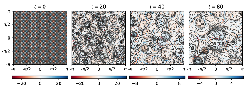
Figure 1: Current density (colors) and magnetic flux (contours) at various times for the run with $S_{0}=1786$.

Numerical Study.

To test the above results, we numerically solve the two-dimensional incompressible Reduced-MHD equations Kadomtsev and Pogutse ; Strauss (1976); Schekochihin et al. (2009) using the pseudo-spectral code Viriato Loureiro et al. (2016). In what follows, quantities are given in dimensionless form. The domain is a periodic square box with sides of length $L=2\pi$. The initial equilibrium is described by the stream function $\phi(x,y)=0$ and the magnetic flux function $\psi(x,y)=\psi_{0}\cos(k_{0}x)\cos(k_{0}y)$, yielding a $2k_{0}\times 2k_{0}$ static array of magnetic islands with opposite polarities (Fig. 1, left panel). In all runs we choose $k_{0}=8$, and thus $R_{0}=L/4k_{0}=\pi/16$. We further set $\psi_{0}k_{0}=1$, implying $B_{0}\equiv\psi_{0}/R_{0}=2/\pi$. This initial equilibrium is perturbed by small-amplitude, spatially random noise to initiate the evolution. We perform a series of runs for different values of resistivity $\eta\in\{1\times 10^{-3},7\times 10^{-4},5\times 10^{-4},3\times 10^{-4},1\times 10^{-4},7\times 10^{-5}\}$, which correspond to the initial island-scale Lundquist number $S_{0}\equiv R_{0}v_{A,0}/\eta\in\{125,179,250,417,1250,1786\}$. Viscosity is set equal to resistivity. We use $8192^{2}$ grid points for $S_{0}=1786$; $4096^{2}$ for $S_{0}=1250,417$; and $2048^{2}$ for $S_{0}=250,179,125$. The widths of initial (SP) current sheets are resolved with 3 or 4 grid points in all cases. Since $S_{0}<10^{4}$ in all runs, reconnection should proceed in the SP regime and no (secondary) plasmoids are expected to arise; visual inspection of our simulations confirms this. Fig. 1 shows the configuration of the system with $S_{0}=1786$ at different times. As expected, island mergers lead to the progressive formation of ever larger structures.

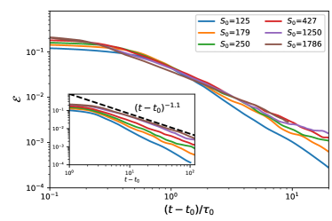
Figure 2: Time evolution of total magnetic energy ($\mathcal{E}$) for all values of $S_{0}$. Time axis in the main figure is normalized to the reconnection timescale $\tau_{0}=S_{0}^{1/2}(\pi^{2}/32)$ (in code units). The inset figure shows same data vs. time in code units. The power-law fit for $S_{0}=1786$ is indicated for reference.

In Fig. 2 we plot the time evolution of the total magnetic energy $\mathcal{E}$ for all values of $S_{0}$. After an initial transient period (represented by a time offset $t_{0}$; for $S_{0}=1786$ it is $t_{0}=4$) the system enters a prolonged stage of self-similar evolution with power-law-in-time behavior; other quantities, such as the number of islands, $N(t)$, or the spatial maximum of the flux, $\psi_{\rm max}(t)$, behave similarly. We fit this data to functions of the form $(t-t_{0})^{\lambda}$. The measured power-law indices, $\lambda_{\mathcal{E}},~{}\lambda_{N}$, and $\lambda_{\psi}$ are found to converge to the predictions of our hierarchical model, Eq. (4), as $S_{0}$ increases, as shown in Fig. 3. This suggests that the hierarchical model can indeed capture the basic dynamics of the merging system. We also find that the time offset $t_{0}$ increases with $S_{0}$, consistent with the expected scaling of the reconnection rate.

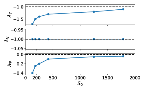
Figure 3: Power-law exponents as functions of initial Lundquist number $S_{0}$. Dashed lines represent the predictions of our model, Eq. (4).

Additionally, Fig. 2 clearly demonstrates that the characteristic timescale for the magnetic energy evolution is the reconnection time, $\tau_{0}$. This is evidenced by the approximate collapse of all curves in the main plot, where the time axis is normalized to $\tau_{0}$, but not in the inset figure, where time is in code units.

Fig. 4 (top panel) shows the magnetic spectrum $U(k,t)$ at different moments of time for the $S_{0}=1786$ run. As is visually intuited from Fig. 1, we observe that the peak of the spectrum moves to larger scales, while retaining an overall similar shape. To the right of the peak, these spectra exhibit power-law behavior (an inertial range), with a slope that is well approximated by the index $\gamma=2$ (in agreement with  Brandenburg et al. (2015); Zrake (2014)). We think that this index is due to the presence of thin current sheets Burgers (1948); indeed, a $k^{-2}$ slope forms even before any coalescence has taken place, and thus it cannot be yielded by the magnetic island distribution. The kinetic energy spectrum (not shown) exhibits a peak at roughly the same wavenumber as the magnetic energy, but follows a shallower power-law, $\sim k^{-1}$. This is consistent with the notion that kinetic energy in the current sheets is dominated by the (Alfvénic) outflows (whose spatial profile Loureiro et al. (2013b) yields a flat spectrum), plus background flows (both inside and outside the magnetic islands) on the scale of the dominant islands.

The self-similarity of the magnetic spectra is clearly demonstrated in the bottom panel of Fig. 4, where we normalize the spectra to their respective maximum values at each moment of time, $U_{\rm max}(t)$, and the wavenumbers to the values $k_{\rm max}(t)$ at which $U_{\rm max}(t)$ are attained. As seen, all curves essentially collapse onto the same distribution, implying that $U(k,t)$ can be factorized as $U(k,t)=U_{\rm max}(t)\bar{U}(k/k_{\rm max})$.

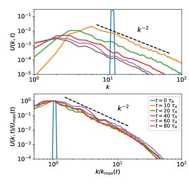
Figure 4: Raw (top) and normalized (bottom) magnetic power spectra, for $S_{0}=1786$. A $k^{-2}$ slope is shown for reference.

We also observe that $k_{\rm max}$ and $U_{\rm max}$ are roughly power-law functions of time, $k_{\rm max}\propto\Delta t^{-\beta}$ and $U_{\rm max}\propto\Delta t^{-\theta}$, where $\Delta t\equiv t-t_{0}$, as shown in the top two panels of Fig. 5. Hence $U(k,t)$ can be expressed as $U(k,t)\propto\Delta t^{-\theta}\bar{U}(k\Delta t^{\beta})$, where $\bar{U}(k/k_{\rm max})$ becomes a universal scaling function of the variable $k\Delta t^{\beta}$, consistent with Eq. (7).

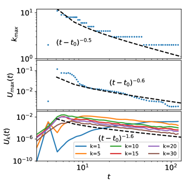
Figure 5: Time evolution of $k_{\rm max}$ (top), $U_{\rm max}$ (middle) and $U_{k}$ (for selected values of $k$; bottom), for $S_{0}=1786$.

As noted above, the spectra exhibit an inertial range [$k>k_{\rm max}(t)$] with a power-law dependence on $k$: $U\propto k^{-\gamma}$ (Fig. 4, top panel). Therefore, in the inertial range, we have the power-law scaling function: $\bar{U}(k\Delta t^{\beta})\propto(k\Delta t^{\beta})^{-\gamma}$, and the power-law time dependence of magnetic spectral energy density at any given $k$: $U_{k}(t)\propto\Delta t^{-\alpha}$ (Fig. 5, bottom panel), leading to the general expression for the spectrum: $U(k,t)\propto k^{-\gamma}\Delta t^{-\alpha}$, where $\alpha=\gamma\beta+\theta$ (see also Zrake (2014)).

The measured values of all the indices as well as the relation between $\alpha$ and $\gamma$, can be compared with our model [Eqs. (7)–(8)]. The results for different simulations are summarized in Table 1, where we also include a $4096^{2}$ simulation performed with hyper-dissipation — this enables us to extend the range of dissipation-free scales as much as possible. We observe that as $S_{0}$ increases, the exponents approach our theoretical predictions.

Lastly, we have performed one run ($\eta=10^{-4},4096^{2}$ grid cells) where the initial condition is instead a Gaussian-random magnetic field, with a spectrum narrowly peaked around $k_{0}=8$. We observe that the power-law exponents obtained in this run are close to those in the run with same $\eta$ but with the periodic-islands initial configuration. This indicates that our reconnection-based hierarchical model can describe the inverse magnetic energy transfer in a more general decaying 2D turbulent system.

$S_{0}$	$\beta$	$\theta$	$\alpha$	$\gamma$
$125$	0.5	1.5	3.0	3.5
$179$	0.6	1.3	2.1	2.9
$250$	0.6	1.3	2.0	2.1
$417$	0.6	1.2	1.9	2.1
$1250$	0.5	1.1	1.8	2.0
$1786$	0.5	0.6	1.6	2.0
Hyper-diss	0.5	0.5	1.5	2.0
Theory	0.5	0.5	1.5	2.0

Table 1: Variation of exponents with initial Lundquist number $S_{0}$, compared with the prediction from the hierarchical model.

Conclusion.

We have introduced a solvable analytic model to describe the inverse transfer of magnetic energy arising from the hierarchical merger of magnetic islands via magnetic reconnection. We have also carried out direct numerical simulations which show good agreement with the predictions of the model, thereby identifying reconnection as the mechanism that sets the properties (including, importantly, the timescale) of such inverse energy transfer. These results — and, more generally, the notion of reconnection as the enabler of inverse energy transfer — are of broad applicability to various space and astrophysical environments. They may, for example, pave the way for understanding the long-term evolution of kinetic-scale seed magnetic fields: a longstanding problem in plasma astrophysics with direct implications to GRBs and galactic magnetogenesis.

References

- Kulsrud and Zweibel (2008) R. M. Kulsrud and E. G. Zweibel, Reports on Progress in Physics 71, 046901 (2008).
- Weibel (1959) E. S. Weibel, Physical Review Letters 2, 83 (1959).
- Gruzinov (2001) A. Gruzinov, The Astrophysical Journal Letters 563, L15 (2001).
- Medvedev and Loeb (1999) M. V. Medvedev and A. Loeb, The Astrophysical Journal 526, 697 (1999).
- (5) W. B. Manchester IV, T. I. Gombosi, I. Roussev, D. L. De Zeeuw, I. V. Sokolov, K. G. Powell, G. Tóth, and M. Opher, Journal of Geophysical Research: Space Physics 109.
- Klimchuk et al. (2008) J. A. Klimchuk, S. Patsourakos, and P. J. Cargill, Astrophys. J. 682, 1351 (2008).
- Khabarova et al. (2015) O. Khabarova, G. Zank, G. Li, J. Le Roux, G. Webb, A. Dosch, and O. Malandraki, The Astrophysical Journal 808, 181 (2015).
- Drake et al. (2012) J. F. Drake, M. Swisdak, and R. Fermo, The Astrophysical Journal Letters 763, L5 (2012).
- Biskamp and Bremer (1994) D. Biskamp and U. Bremer, Physical Review Letters 72, 3819 (1994).
- Olesen (1997) P. Olesen, Physics Letters B 398, 321 (1997).
- Biskamp and Schwarz (2001) D. Biskamp and E. Schwarz, Physics of Plasmas 8, 3282 (2001).
- Zrake (2014) J. Zrake, The Astrophysical Journal Letters 794, L26 (2014).
- Brandenburg et al. (2015) A. Brandenburg, T. Kahniashvili, and A. G. Tevzadze, Physical Review Letters 114, 075001 (2015).
- Zrake and East (2016) J. Zrake and W. E. East, The Astrophysical Journal 817, 89 (2016).
- Medvedev et al. (2004) M. V. Medvedev, M. Fiore, R. A. Fonseca, L. O. Silva, and W. B. Mori, The Astrophysical Journal Letters 618, L75 (2004).
- Kato (2005) T. N. Kato, Physics of plasmas 12, 080705 (2005).
- Katz et al. (2007) B. Katz, U. Keshet, and E. Waxman, The Astrophysical Journal 655, 375 (2007).
- Fermo et al. (2010) R. Fermo, J. Drake, and M. Swisdak, Physics of Plasmas 17, 010702 (2010).
- (19) 83.
- Finn and Kaw (1977) J. M. Finn and P. Kaw, The Physics of Fluids 20, 72 (1977).
- Sweet (1958) P. A. Sweet, in Electromagnetic Phenomena in Cosmical Physics, IAU Symposium, Vol. 6, edited by B. Lehnert (1958) p. 123.
- Parker (1957) E. N. Parker, Journal of Geophysical Research 62, 509 (1957).
- Loureiro et al. (2007) N. F. Loureiro, A. A. Schekochihin, and S. C. Cowley, Physics of Plasmas 14, 100703 (2007).
- Lapenta (2008) G. Lapenta, Physical Review Letters 100, 235001 (2008).
- Samtaney et al. (2009) R. Samtaney, N. F. Loureiro, D. A. Uzdensky, A. A. Schekochihin, and S. C. Cowley, Physical Review Letters 103, 105004 (2009).
- Bhattacharjee et al. (2009) A. Bhattacharjee, Y.-M. Huang, H. Yang, and B. Rogers, Physics of Plasmas 16, 112102 (2009).
- Huang and Bhattacharjee (2010) Y.-M. Huang and A. Bhattacharjee, Physics of Plasmas 17, 062104 (2010).
- Uzdensky et al. (2010) D. A. Uzdensky, N. F. Loureiro, and A. A. Schekochihin, Physical Review Letters 105, 235002 (2010).
- Loureiro et al. (2012) N. F. Loureiro, R. Samtaney, A. A. Schekochihin, and D. A. Uzdensky, Physics of Plasmas 19, 042303 (2012).
- Loureiro et al. (2013a) N. F. Loureiro, A. A. Schekochihin, and A. Zocco, Physical Review Letters 111, 025002 (2013a).
- Loureiro and Uzdensky (2016) N. F. Loureiro and D. A. Uzdensky, Plasma Physics and Controlled Fusion 58, 014021 (2016).
- Note (1) In the collisionless case Cassak et al. (2017) should also remain constant in time, even though the reconnection regime transitions from laminar to plasmoid-mediated as grows while the ion skin depth remains constant Ji and Daughton (2011) — though the efficiency of coalescence may be decreased Karimabadi et al. (2011); Stanier et al. (2015).
- Biskamp and Welter (1989) D. Biskamp and H. Welter, Physics of Fluids B: Plasma Physics 1, 1964 (1989).
- (34) P. Olesen, arXiv preprint arXiv:1509.08962 .
- Burgers (1948) J. M. Burgers, in Advances in applied mechanics, Vol. 1 (Elsevier, 1948) pp. 171–199.
- (36) B. Kadomtsev and O. Pogutse, Sov. Phys. JETP 5, 575.
- Strauss (1976) H. R. Strauss, The Physics of Fluids 19, 134 (1976).
- Schekochihin et al. (2009) A. A. Schekochihin, S. C. Cowley, W. Dorland, G. W. Hammett, G. G. Howes, E. Quataert, and T. Tatsuno, The Astrophysical Journal Supplement Series 182, 310 (2009).
- Loureiro et al. (2016) N. F. Loureiro, W. Dorland, L. Fazendeiro, A. Kanekar, A. Mallet, M. Vilelas, and A. Zocco, Computer Physics Communications 206, 45 (2016).
- Note (2) The number of islands is numerically determined by diagnosing the O-points and X-points of the system, identified with the maximum/minimum and saddle points of (e.g., Servidio et al., 2009).
- Loureiro et al. (2013b) N. F. Loureiro, A. A. Schekochihin, and D. A. Uzdensky, Physical Review E 87, 013102 (2013b).
- Note (3) We also observe in our simulations that kinetic energy decays as , consistent with .
- Cassak et al. (2017) P. Cassak, Y.-H. Liu, and M. Shay, Journal of Plasma Physics 83 (2017).
- Ji and Daughton (2011) H. Ji and W. Daughton, Physics of Plasmas 18, 111207 (2011).
- Karimabadi et al. (2011) H. Karimabadi, J. Dorelli, V. Roytershteyn, W. Daughton, and L. Chacón, Physical Review Letters 107, 025002 (2011).
- Stanier et al. (2015) A. Stanier, W. Daughton, L. Chacon, H. Karimabadi, J. Ng, Y.-M. Huang, A. Hakim, and A. Bhattacharjee, Physical Review Letters 115, 175004 (2015).
- Servidio et al. (2009) S. Servidio, W. H. Matthaeus, M. A. Shay, P. A. Cassak, and P. Dmitruk, Physical Review Letters 102, 115003 (2009).