On integrands and loop momentum in string and field theory

Abstract

The notion of a unique integrand does not a priori makes sense in field theory: different Feynman diagrams have different loop momenta and there should be no reason to compare them. In string theory, however, a global integrand is natural and allows, for instance, to make explicit the separation between left and right-moving degrees of freedom.

However, the significance of this integrand had not really been investigated so far. It is even more important in view of the recently discovered loop monodromies that are related to the duality between color and kinematics in gauge and gravity loop amplitudes.

This paper intends to start filling this gap, by presenting a careful definition of the loop momentum in string theory, and describing precisely the resulting global integrand obtained in the field theory limit. We will then apply this technology to write down some monodromy relations at two and three loops, and make contact with the color/kinematics duality.

1 Introduction

In the last few years, a variety of results for scattering amplitudes in field theory at loop-level have been derived using string theoretic methods. Interestingly, many of them have focused on integrands and have involved explicit dependence on a loop momentum defined globally for a string integrand.

While this is a peculiar idea from a traditional Feynman perspective, this concept is actually present, though maybe not emphasised, since the very early days of string theory Shapiro:1972ph . The seminal papers Verlinde:1986kw ; Verlinde:1987sd ; DHoker:1988pdl ; DHoker:1989cxq then laid the foundations for the definition of the loop momentum in string theory amplitudes in their modern formulation as conformal field theory correlation functions integrated over the moduli space of Riemann surfaces. Those correlation functions can be written as holomorphic squares in loop amplitudes only in presence of loop momentum. Especially non-trivial for superstrings (in the RNS formulation), this property was called chiral splitting.

However, some aspects related to the precise definition of the loop momentum had not been worked out and the recent results alluded to above require to now re-investigate this question. I have especially in mind two categories of results: the monodromy relations at higher loops in string theory derived in Tourkine:2016bak and the scattering equation or ambitwistor string methods at loop level. This paper will be focussed on the former, I allude to the latter in the discussion.

The monodromy relations in string theory were originally derived at tree-level Plahte:1970wy ; BjerrumBohr:2009rd ; Stieberger:2009hq . They are now understood to generalize of the Bern-Carrasco-Johanson Bern:2008qj (BCJ) duality between colour and kinematics that underlie the so-called double-copy construction Bern:2010ue of gravity integrands as squares of Yang-Mills integrands. While implemented very efficiently to compute loop amplitudes, see for instance the last recent achievement at five loops and references therein Bern:2018jmv , this duality is still not understood from first principles.

The tree-level relations were extended to all loop orders in Tourkine:2016bak in open string theory. This gives hope that string theory can shed light on the colour-kinematics duality and these relations need to be understood deeper. In particular, some aspects related to the definition of the loop momentum were only conjectured in Tourkine:2016bak and the present paper intends to fill this gap and show in details how to apply the monodromy relations at higher loops.

Another aspect that this paper deals with is the notion of an integrand in field theory. In Tourkine:2016bak , it was emphasized that the relations induced in field theory by the stringy monodromies are valid globally at the integrand level, i.e. mix different integrands of different graphs at the same value of the loop momentum, as in Chiodaroli:2017ngp . We will see how this picture generically emerges from the field theory limit of string amplitudes.

Here is a summary of the main contributions of this paper:

1. A precise definition of the loop momentum in the string theory integrand in 2, from a review of classic computations and from solving directly the classical equations of motion for the string. The definition requires working on a so-called canonical dissection of the surface (see fig. 1), which, importantly, breaks modular invariance DHoker:1988pdl because it does not allow to modify the homology basis anymore.

2. A careful study of its field theory limit (in sec. 2, which as a by-product gives how the loop momentum is distributed across all Feynman graphs appearing in this limit. This analysis uses some tools to study the degeneration of Riemann surfaces.

3. Finally I provide applications of these definitions in loop amplitudes. In particular, we shall see in details how the monodromy relations work two and three-loop amplitudes, which support further the claim that the monodromy relations generalize the BCJ duality. More precisely it will support the conjecture that in all higher loop relations, the monodromy relations always combine the numerators appearing in the field theory limit into groups of graphs called BCJ triplets.

It should be noted that in this paper we will exclusively be concerned with the bosonic part of the string amplitudes, which is the one that carries the loop-momentum zero modes.

Further applications of these results are presented in the discussion 5 together with open questions.

2 String theory

The presence of loop momentum is standard in the operator formalism of the string theory, this is for instance the was that amplitudes are derived in the classic book by Green Schwarz and Witten Green:2012pqa . These representations have the advantage to make chiral splitting manifest DHoker:1989cxq , i.e. the string integrand is factorized as a product of a purely left-moving (holomorphic) and right-moving (anti-holomorphic) part. The traditional form of the string amplitudes is obtained after integrating out the loop-momentum, which induces non-holomorphy in the integrand and destroys its chiral splitting.

The drawback, however, is that this formalism is difficult to use at high multiplicity and loop orders because it amounts to do a very complicated Feynman diagram computation, and the number of graphs increases quickly. Besides, the structure of the moduli space of Riemann surfaces at higher genus essentially renders the whole process unusable. The modern approach to string theory scattering amplitudes is based on complex (super)-geometry and conformal field theory techniques DHoker:1988pdl . In this manner, the non-holomorphic terms are generated from the start Verlinde:1986kw ; Verlinde:1987sd ; DHoker:1988pdl ; DHoker:1989cxq , essentially because meromorphic functions on Riemann surfaces must have the sum of their residues vanishing (via Stoke’s theorem). We review this construction now.

We will review the construction of the universal part to string theory amplitudes at loop-level. It is the generalisation of the Koba-Nielsen factor $\prod_{i<j}|z_{i}-z_{j}|^{\alpha^{\prime}k_{i}\cdot k_{j}}$ ubiquitous to tree-level string amplitudes. Here and throughout, $z_{i}$ will be the locations of the vertex operators on the string worldsheet, $\alpha^{\prime}$ is the string Regge slope, and $k_{i}$ are null momenta of the states, all taken to be incoming, that satisfy momentum conservation $\sum_{i=1}^{n}k_{i}=0$ for and $n$-particle process.

Along the way we shall see how the loop momentum appears. We will mostly follow DHoker:1988pdl , and supplement the construction with careful normalisations and definitions of the loop-momentum. Note that the paper Skliros:2016fqs presents details on these computations and an exhaustive reference list on the matter.

In the conformal gauge, the Polyakov action for closed strings reads

$$S_{\mathrm{P}}=\frac{1}{2\pi\alpha^{\prime}}\int_{\Sigma}\partial_{z}X\partial_{\bar{z}}X\,.$$ (1)

where $X^{\mu}(z,\bar{z})$ are the coordinates of the string in $d$-dimensional target flat space.

The equations of motion of the theory without vertex operator insertions split the $X$ field into left and right-movers as

$$X^{\mu}(z,\bar{z})=X_{L}^{\mu}(z)+X_{R}^{\mu}(\bar{z})$$ (2)

which will share a common zero mode $x_{L}=x_{R}$ and a loop momentum zero mode to be introduced momentarily.

In the presence of $n$ standard exponential vertex operator insertions,

$$V_{j}(k_{j})=\exp(ik_{j}\cdot X(z_{j},\bar{z}_{j}))$$ (3)

the phases can be inserted in the action and the object we seek to compute is given by:

$$\langle\!\langle\,V_{1}(k_{1})\dots V_{n}(k_{n})\,\rangle\!\rangle=\int\mathcal{D}Xe^{-\frac{1}{2\pi\alpha^{\prime}}\int d^{2}z\partial_{z}X^{\mu}\partial_{\bar{z}}X_{\mu}+2i\pi\alpha^{\prime}\sum_{j=1}^{n}k_{j}^{\mu}X_{\mu}(z,\bar{z})\delta^{2}(z-z_{i})d^{2}z}$$ (4)

where the double bracket notation is that of DHoker:1988pdl . To compute this path integral, we need to invert the kinetic operator $\partial_{z}\partial_{\bar{z}}$, i.e. compute the Green’s function

$${G}(z,w)\eta^{\mu\nu}=\langle X(z,\bar{z})^{\mu}X(w,\bar{w})^{\nu}\rangle\,.$$ (5)

The subtlety when doing this directly comes from the fact that $\partial_{z}$ and $\partial_{\bar{z}}$ have zero modes on a compact Riemann surface $\Sigma$ of genus $g\geq 1$, that correspond to loop momentum. They are supported by $g$ holomorphic and anti-holomorphic one-forms $\omega_{I}$ and $\bar{\omega}_{J}$ that span the cohomologies $H^{(1,0)}(\Sigma)$ and $H^{(0,1)}(\Sigma)$ :

$$\forall I=1\dots g,\quad\partial\bar{\omega}_{I}=0,\quad\bar{\partial}\omega_{I}=0\,.$$ (6)

In this equation and below, $\partial$ and $\bar{\partial}$ are operators $\partial=(\partial/\partial z)dz$ and $\bar{\partial}=(\partial/\partial\bar{z})d\bar{z}$, as defined in appendix A. We also abbreviate $\partial_{z}:=(\partial/\partial z)$ and likewise for $\partial_{\bar{z}}$.

The holomorphic one-forms are dual to a homology of one-cycles, traditionally called $a$ and $b$ cycles, canonically defined by their intersection numbers $a_{I}\cap b_{J}=\delta_{I,J}$, for $I,J=1\dots g$, all other vanishing. Pairing a cycle with a form is done via the period map $(\omega,c)\mapsto\int_{c}\omega$. Normalising the period of the 1-forms on the $a_{I}$ cycles to $\delta_{IJ}$ makes the periods along the $b$ cycles define the period matrix $\Omega$ of the surface as follows

$$\oint_{a_{I}}\omega_{J}=\delta_{IJ}\,,\qquad\oint_{b_{I}}\omega_{J}=\Omega_{IJ}\,.$$ (7)

It is a symmetric $g\times g$ matrix with positive-definite imaginary part $\,\textrm{Im}\,\Omega>0$.

Let us then fix a Riemann surface $\Sigma$ of genus $g$. The kinetic operator can be inverted on the space orthogonal to the zero modes Verlinde:1986kw ; Verlinde:1987sd ; DHoker:1988pdl and the equations that define the corresponding Green’s function are

$$\int_{\Sigma}G(z,w)d^{2}z=0\,,$$ (8)

$$\partial_{z}\partial_{\bar{z}}G(z,w)=-2\pi\alpha^{\prime}\delta^{2}(z-w)+\frac{2\pi\alpha^{\prime}}{\int d^{2}z\sqrt{g}}\,,$$ (9)

$$\partial_{z}\partial_{\bar{w}}=2\pi\alpha^{\prime}\delta^{(2)}(z-w)-{\alpha^{\prime}\pi}\sum_{I,J}\omega_{I}(z)(\,\textrm{Im}\,\Omega)^{-1}_{IJ}\bar{\omega}_{J}(w)\,.$$ (10)

where $g$ is the determinant of the metric on the surface, as defined in A. These equations can be solved and yield

$${G}(z_{1},z_{2})=-\frac{\alpha^{\prime}}{2}\ln\left(|E(z_{1},z_{2})|^{2}\right)+\alpha^{\prime}\pi\,\textrm{Im}\,\left(\int_{z_{2}}^{z_{1}}{\omega_{I}}\right)((\,\textrm{Im}\,\Omega)^{-1})^{IJ}\,\textrm{Im}\,\left(\int_{z_{2}}^{z_{1}}{\omega_{J}}\right)\,.$$ (11)

up to terms which we neglect because vanish on the support of momentum conservation. The prime form $E$ is defined in (72). Its essential property is that it vanishes linearly on the diagonal

$$E(x,y)=x-y+O(x-y)^{3}.$$

It is defined on the universal cover of $\Sigma$, because it has monodromies (given in eq. (74)) along $a$ and $b$ cycles transportation. The non-holomorphic correction in eq. (11) exactly cancels these monodromies and the Green’s function is correctly defined on the surface and not its cover.

The correlation function (4) is then computed by Wick’s theorem:

$$\langle\prod_{i=1}^{n}e^{ik_{i}X(z_{i},\bar{z}_{i})}\rangle=e^{-\sum_{i<j}k_{i}\cdot k_{j}G(z_{i},z_{j})}$$ (12)

Because of the non-holomorphic terms, this expression cannot be written as it stands as a modulus square. Note that they are absent at tree-level,

$$\langle X^{\mu}(z_{1},\bar{z}_{1})X^{\nu}(z_{2},\bar{z}_{2})\rangle=-\frac{\alpha^{\prime}}{2}\eta^{\mu\nu}\ln(|z_{1}-z_{2}|^{2})$$ (13)

and the correlator (12) can be chirally split. At loops, where the $\ln|E|^{2}$ term similarly poses no problem: in the exponential of (12) the problematic terms are

$$Q_{\mathrm{NH}}=\alpha^{\prime}\pi\sum_{i<j}k_{i}\cdot k_{j}\,\textrm{Im}\,\left(\int_{z_{j}}^{z_{i}}{\omega_{I}}\right)((\,\textrm{Im}\,\Omega)^{-1})^{IJ}\,\textrm{Im}\,\left(\int_{z_{j}}^{z_{i}}{\omega_{J}}\right)$$ (14)

Let $P$ be a point on the surface, so that we can decompose the integration $\int_{z_{j}}^{z_{i}}$ as $\int_{z_{j}}^{P}+\int_{P}^{z_{i}}$, (14) then becomes

$$Q_{NH}=\alpha^{\prime}\pi\sum_{i<j}k_{i}\cdot k_{j}\,\textrm{Im}\,\left(\int_{z_{j}}^{P}+\int_{P}^{z_{i}}{\omega_{I}}\right)((\,\textrm{Im}\,\Omega)^{-1})^{IJ}\,\textrm{Im}\,\left(\int_{z_{j}}^{P}+\int_{P}^{z_{i}}{\omega_{J}}\right)$$ (15)

The diagonal terms $\,\textrm{Im}\,\int_{P}^{z_{i}}\omega_{I}((\,\textrm{Im}\,\Omega)^{-1})^{IJ}\,\textrm{Im}\,\int_{P}^{z_{i}}\omega_{J}$ vanish by momentum conservation (summing over $j$ in this case), so we keep only the crossed terms and we would want to rewrite (15) as

$$Q_{NH}=-2\pi\alpha^{\prime}\sum_{i<j}k_{i}\cdot k_{j}\,\textrm{Im}\,\left(\int_{P}^{z_{j}}{\omega_{I}}\right)((\,\textrm{Im}\,\Omega)^{-1})^{IJ}\,\textrm{Im}\,\left(\int_{P}^{z_{i}}{\omega_{J}}\right)$$ (16)

(the sign comes from flipping the orientation of the integration in one term). The reason why this identity is not straightforward is because it is valid if and only if all the paths from $P$ to $z_{i}$ need to be uniquely defined. Hence, we are looking for a way to define uniquely, for all values of $z_{i}$ on $\Sigma$, a path from $P$ to $z_{i}$. Ambiguities can arise from $z$ winding along a non-trivial cycles, and therefore what we describe is a way to cut open the Riemann surface into a polygon with $4g$ faces, called its canonical dissection, as in fig. 1. It is defined by cutting open the surface along the $a$ and $b$ cycles, not considered anymore as representatives in the homology, but as actual curves, all of which touching in one point exactly.

Figure 1: Canonical dissection along the homology cycles.

Now, because the sum is factorized in (16), we can introduce a Gaussian $d$-dimensional integration so that

$$(\det\,\textrm{Im}\,\Omega)^{d/2}\int\frac{d^{D}\ell}{(2\pi)^{D}}e^{-\pi\alpha^{\prime}\ell_{I}\ell_{J}\,\textrm{Im}\,\Omega^{IJ}-2\pi\alpha^{\prime}\sum_{i,J}\ell_{J}\cdot k_{i}\,\textrm{Im}\,\int_{P}^{z_{i}}\omega_{J}}=\\ e^{2\pi\alpha^{\prime}\sum_{i<j}k_{i}\cdot k_{j}\,\textrm{Im}\,(\int^{z_{j}}_{P}{\omega_{I}})((\,\textrm{Im}\,\Omega)^{-1})^{IJ}\,\textrm{Im}\,(\int_{P}^{z_{i}}{\omega_{J}})}$$ (17)

up to a global normalisation factor. Using that $\exp(-2\,\textrm{Im}\,x)=|\exp(x)|^{2}$, this expression can be further rewritten as a modulus square, and finally we have

$$\langle\!\langle\,V_{1}(k_{1})\dots V_{n}(k_{n})\,\rangle\!\rangle=\int\frac{d^{d}\ell}{(2\pi)^{d}}\langle\!\langle\,V_{1}(k_{1})\dots V_{n}(k_{n})\,\rangle\!\rangle(\ell_{I})$$ (18)

where

$$\langle\!\langle\,V_{1}(k_{1})\dots V_{n}(k_{n})(\ell_{I})\,\rangle\!\rangle=(\,\textrm{Im}\,\Omega)^{d/2}\bigg{|}e^{\tfrac{i\pi\alpha^{\prime}}{2}\ell_{I}\ell_{J}\Omega^{IJ}+i\pi\alpha^{\prime}\sum_{i,J}\ell_{J}\cdot k_{i}\int_{P}^{z_{i}}\omega_{J}}\prod_{i,j}{E(z_{i},z_{j})}^{\alpha^{\prime}k_{i}k_{j}/2}\bigg{|}^{2}\,\,$$ (19)

which is eq.(2.99) of DHoker:1988pdl . This is the content of chiral splitting for the bosonic part of the amplitudes.

The most important conclusion of this section is that the loop momenta are defined with respect to a specific canonical dissection, and not just the homology. Now we will see how this can be derived from looking at the classical trajectory for the field $X$; this will lead to a precise definition of the momentum flowing through a given cycle.

A consequence of working on a canonical dissection is that modular invariance (the freedom to change $a$ and $b$ cycles) is totally broken, because $a$ and $b$ cycles cannot be mixed anymore within the string integrand. Of course, re-integrating out the loop momentum gives modular invariant expressions.

Classical solution.

Since the action is free, all those quantities could have been equivalently computed from the classical solution of the Euler-Lagrange equation with sources. For $X$, it can be obtained by varying the action (4) or, equivalently, by computing

$$X_{\mathrm{class}}^{\mu}(z,\bar{z})=\frac{\langle X^{\mu}(z,\bar{z})\prod_{i=1}^{n}e^{ik_{i}X(z_{i},\bar{z}_{i})}\rangle}{\langle\prod_{i=1}^{n}e^{ik_{i}X(z_{i},\bar{z}_{i})}\rangle}$$ (20)

using the individual two-point functions $\langle XX\rangle$.

Let us follow the former approach. We want to minimize the following action

$$S=\frac{1}{2\pi\alpha^{\prime}}\int_{\Sigma}\partial_{z}X\partial_{\bar{z}}X+2i\pi\alpha^{\prime}\sum_{j}k_{j}^{\mu}X(z,\bar{z})\delta^{2}(z-z_{i},\bar{z}-\bar{z}_{i})\,.$$ (21)

It is instructive to first do the computation at tree-level when there are not yet zero modes. The $\frac{\delta}{\delta X}$ variation of this Lagrangian yields

$$2\partial_{z}\partial_{\bar{z}}X^{\mu}=2i\pi\alpha^{\prime}\sum_{i}k_{i}^{\mu}\delta^{2}(z-z_{i},\bar{z}-\bar{z}_{i})$$ (22)

Using that

$$\partial_{\bar{z}}\frac{1}{z}=\partial_{z}\frac{1}{\bar{z}}=2\pi\delta^{(2)}(z,\bar{z})\,,$$ (23)

this integrates once to

$$\partial_{\bar{z}}X^{\mu}=\frac{i\alpha^{\prime}}{2}\sum_{i}\frac{k_{i}^{\mu}}{\bar{z}-\bar{z}_{i}}$$ (24)

and then

$$X_{\mathrm{class}}^{\mu}=x_{R}+\frac{i\alpha^{\prime}}{2}\sum_{i}k_{i}^{\mu}\ln(\bar{z}-\bar{z}_{i})+X_{L}(z)\,.$$ (25)

The holomorphic part is determined by re-injecting this equation in the equations of motion and one finds

$$X_{\mathrm{class}}^{\mu}=x_{0}+\frac{i\alpha^{\prime}}{2}\sum_{i}\ln|z-z_{i}|^{2}$$ (26)

where $x_{0}=x_{L}+x_{R}$ is the zero-mode that gives rise to momentum conservation upon $\int d^{d}x_{0}$ integration.

Let us now go to loop level and consider a Riemann surface $\Sigma$ of genus $g$. Analogously to the tree-level case, we can obtain the singular part of $\partial X^{\mu}_{L}(z)$ in terms of meromorphic differentials with single poles $\omega_{z_{+},z_{-}}=\omega_{z_{+},z_{-}}(z)dz$ with residue $\pm 1$ at $z=z_{\pm}$. They are called abelian differentials of third kind and can be uniquely defined by normalising to zero their periods along the $a$-cycles:

$$\omega_{z_{+},z_{-}}(z)\underset{z\to z_{\pm}}{\sim}\pm\frac{1}{z-z_{\pm}};\qquad\forall I=1\dots g,\quad\oint_{a_{I}}\omega_{z_{+},z_{-}}=0\,.$$ (27)

For further convenience, let us denote $c_{i}$ the circles $|z-z_{i}|=\epsilon$. This allows to define a singular homology on $\Sigma-\{z_{1},\dots,z_{n}\}$ by augmenting that of $\Sigma$ with these $n$ new $c$ cycles.

The new ingredient compared to the tree-level case is the presence of zero-modes for the $\bar{\partial}$ and $\partial$ operators, given by the holomorphic one-forms and their complex conjugates, as in (6). After the first integration of (22), we find

$$\partial X^{\mu}_{L}(z)=i\pi\alpha^{\prime}\sum_{J=1}^{g}\omega_{J}\ell_{J}^{\mu}+\frac{i\alpha^{\prime}}{2}\sum_{i=1}^{n}\omega_{z_{i},z_{0}}k_{i}^{\mu}$$ (28)

$$\bar{\partial}X^{\mu}_{R}(\bar{z})=i\pi\alpha^{\prime}\sum_{J=1}^{g}\bar{\omega}_{J}\tilde{\ell}_{J}^{\mu}+\frac{i\alpha^{\prime}}{2}\sum_{i=1}^{n}\bar{\omega}_{z_{i},z_{0}}k_{i}^{\mu}$$ (29)

where $z_{0}$ is an extra variable whose dependence drops out by momentum conservation. I left unspecified the zero modes for the holomorphic and anti-holomorphic fields, they will be fixed later by physical requirement of measure a correctly normalised momentum. Integrating once more gives

$$X_{L,\mathrm{class}}^{\mu}(z)=x_{L}^{\mu}+i\pi\alpha^{\prime}\sum_{J=1}^{g}\ell_{J}^{\mu}\int_{P}^{z}\omega_{J}+\frac{i\alpha^{\prime}}{2}\sum_{i=1}^{n}k_{i}^{\mu}\int_{P}^{z}\omega_{z_{i},z_{0}}$$ (30)

$$X_{R,\mathrm{class}}^{\mu}(\bar{z})=x_{R}^{\mu}+i\pi\alpha^{\prime}\sum_{J=1}^{g}\tilde{\ell}_{J}^{\mu}\int_{P}^{\bar{z}}\bar{\omega}_{J}+\frac{i\alpha^{\prime}}{2}\sum_{i=1}^{n}k_{i}^{\mu}\int_{P}^{\bar{z}}\bar{\omega}_{z_{i},z_{0}}$$ (31)

Finally, $X_{\mathrm{class}}^{\mu}$ is given by the sum of these two equations. To make contact with the previous derivation and eq. (19) in particular, note that the prime form is related to the abelian differentials of the third kind by

$$\partial_{z}\ln\left(\frac{E(z,a)}{E(z,b)}\right)=\omega_{a,b}(z)$$ (32)

This also defines uniquely the zero modes of $\partial X,\bar{\partial}X$ with correct normalisation. To measure the loop momentum flowing through a typical cycle $C$, which is a combination of the canonical $a_{J}$ cycles and $c_{i}$ cycles, we define the following flux

$$P_{C}^{\mu}=\frac{1}{2\pi\alpha^{\prime}}\oint_{C}(-\partial_{z}dz+\partial_{\bar{z}}d\bar{z})X$$ (33)

The normalisation is fixed in a first stage by demanding that integration along $c_{i}$ cycles provides momentum $k_{i}$:

$$\frac{1}{2\pi\alpha^{\prime}}\oint_{c_{i}}(-\partial_{z}dz+\partial_{\bar{z}}d\bar{z})X^{\mu}=k_{i}^{\mu}\frac{i\alpha^{\prime}}{4\pi\alpha^{\prime}}\oint_{c_{i}}(-\omega_{z_{i},z_{0}}+\bar{\omega}_{z_{i},z_{0}})=k_{i}^{\mu}$$ (34)

Then we have

$$\frac{1}{2\pi\alpha^{\prime}}\oint_{a_{I}}(-dz\partial_{z}+d\bar{z}\partial_{\bar{z}})X^{\mu}=-\delta_{IJ}i(\ell_{J}^{\mu}-\tilde{\ell}_{J}^{\mu})/2\equiv\ell_{I}^{\mu}$$ (35)

if the loop momenta are taken to be purely imaginary. This derivation gives another check of this property which was originally observed in DHoker:1988pdl ; DHoker:1989cxq and that seems fundamental to string theory on euclidean worldsheets. It would be interesting to study the consequences of this fact in the ambitwistor string where a similar normalisation was observed to arise by matching against field theory computations in Casali:2014hfa .

Open strings on orientable surfaces are obtained by modding out by the involution $z\simeq\bar{z}$ along the $a$-cycles of the string worldsheet Bianchi:1989du and letting the punctures live on the boundary of the surfaces. More precisely, if $z=\rho e^{i\theta}$ with $\theta\in[0,2\pi[$ is a local coordinate along an $a$ cycle, we identify $\theta\leftrightarrow-\theta$. This is the natural involution to describe the gauge theory channel of open string amplitudes, which we will use later to apply the monodromy relations in open string theory and their induced relations in field theory. This involution can also be used to obtain some non-planar graphs, as long as they are given by orientable surfaces.

Note also that this turns the cycles of the canonical dissection into segments on the worldsheet such that $\oint_{a_{I}}\omega_{J}\to\int_{a_{I}^{\prime}}\omega_{J}=\delta_{IJ}/2$ where $a_{I}^{\prime}$ is $a_{I}$ modulo the involution.

3 Field theory integrand.

In this section we will investigate one implication of the previous considerations. Since there exists a global integrand in string theory, there needs to exist one in field theory, induced via the field theory limit. In practice, after studying the field theory limit itself, we will be able to describe the graph integrand topologies: external leg ordering, and labeling of the internal loop momenta.

The understanding of the mechanism of the field theory limit of string graphs is almost as old as string theory itself Scherk:1971xy . It is produced by corners of the moduli space where the surface degenerate so that all internal edges become infinitely long and thin (this is a $b$-cycle statement) or equivalently where all $a$ and $c$-cycles are pinched. This is a continuous process, known in the maths literature as a tropical limit Tourkine:2013rda .

The property which we will need to describe the graphs loop-momentum-labeling is that the momentum flowing through a cycle is preserved by the field theory limit. As the momentum is a zero-mode, it is not affected by the decoupling of the excited states of the string, therefore the result which we seek for is physically sound and the problem reduces to a computational matter.

Figure 2: From the picture we see that $C\cup(a_{2})^{-1}\cup b_{1}\cup(b_{1})^{-1}\cup c_{1}\cup c_{2}=\mathrm{id}$, hence $C=a_{2}\cup(c_{1})^{-1}\cup(c_{2})^{-1}$ and the momentum flowing through $C$ is given by $\frac{1}{2\pi\alpha^{\prime}}\oint_{C}(-\partial+\bar{\partial})X^{\mu}=\ell_{2}^{\mu}-k_{1}^{\mu}-k_{2}^{\mu}$.

Let $C$ be a closed curve made of $a_{I}$- and $c_{i}$-cycles:

$$C=\cup_{i\in\mathcal{I}_{C}}\mathbf{a}_{i}$$ (36)

where $\mathbf{a}$ is either a $a$ cycle or a $c$ cycle with coefficient $1$. This defines implicitly the set $\mathcal{I}_{C}$. This excludes the possibility that our cycle $C$ could wind multiple times. For illustrative purposes, see fig. 2. Let us call the corresponding momentum

$$p_{C}^{\mu}=-\frac{1}{2\pi\alpha^{\prime}}\oint_{C}(dz\partial_{z}-d\bar{z}\partial_{\bar{z}})X=\sum_{I,i\in\mathcal{I}_{C}}(\ell_{I}^{\mu}+k_{i}^{\mu})$$ (37)

with obvious notations for the summation. The crucial point is that this quantity is a topological invariant, therefore it cannot change as we deform continuously the surface when taking the field theory limit. We now will check this property and see that when the $C$ cycle degenerates, as in fig. 5 and show that a propagator $1/p_{C}^{2}$ factorizes out of the string amplitude.

3.1 Single pinching of a Riemann surface.

There are two types of degenerations that a Riemann surface can undergo: separating and non-separating. The separating degeneration corresponds to pinching off a trivial cycle in the homology or a $c$-cycle: it splits appart a surface of genus $g$ into two surfaces of genera $g_{1}$ and $g_{2}$ such that $g=g_{1}+g_{2}$. A non-separating degeneration pinches off an $a$-type cycle and the resulting object is a surface with genus decreased by one unit and two extra punctures. This is the case of interest for us because we want to check that a propagator with expected loop momentum labeling is generated. An example of such a degeneration is provided in fig.5.

Firstly, let us observe that we do not loose in generality by considering that the $a$ cycle part of our $C$ cycle is the cycle $a_{g}$ (we could always relabel the $a$ cycles).

The degeneration of the Riemann surface is done via the so-called plumbing fixture construction see Fay or DHoker:1988pdl ; DHoker:2017pvk . In this construction, the degenerating curve $\Sigma_{g}$ is constructed from a Riemann surface of genus $g-1$, $\Sigma_{g-1}$ with period matrix $\Omega_{g-1}$ and a pair of points marked on the surface $p_{a}$ and $p_{b}$. To construct $\Sigma_{g}$, one constructs two pairs of circles centered around $p_{a}$ and $p_{b}$: $C_{a}^{\prime\prime}$ and $C_{b}$’ of radius 1 and $C_{a}^{\prime},C_{b}^{\prime\prime}$ of radius $|q|<1$ for complex number $q$ that parametrizes the degeneration. The internal disk is then cut out of the surface and the annuli between the disks are identified via an invertible map

$$xy=q\,.$$

The extra $a$ cycle $a_{g}$ is a closed loop around $C_{a}^{\prime\prime}$ for instance; the extra $b$ cycle $b_{g}$ is a line that connects any two points $z_{a}$ and $z_{b}$ in the annuli that obey $z_{a}z_{b}=q$. Choosing $|z_{a}|=|z_{b}|=\sqrt{|q|}$ ensures that when $q=0$, the extra cycle is really the line connecting the two points $p_{a}$ and$p_{b}$ which are identified.

Figure 3: Illustration of the plumbing fixture construction.

Then, if $\Omega_{g}$ is the period matrix of $\Sigma_{g}$, Fay in Fay proves that

$$\Omega_{g}\sim\left(\begin{array}[]{@{}c|c@{}}\mbox{ $\Omega_{g-1}$ \phantom{\bigg{|}}}&\vec{v}\\ \hline\cr\vec{v}{\,}^{t}&\tau\end{array}\right)\,,\quad\mathrm{where~{}}q=e^{2i\pi\tau}\,,$$ (38)

up to sub-leading terms and where the components of $\vec{v}$ are given by $v_{I}=\int_{p_{a}}^{p_{b}}\omega_{I}^{(g-1)}$, $I=1\dots g-1$. The exponent on the differential form $\omega_{I}^{(h)}$ designate the surface $\Sigma_{h}$ to which it is associated for $h=g,g-1$.

With this, we can already extract the degeneration of the quadratic term in the loop momentum in the exponential in eq.(19):

$$\sum_{I,J=1}^{g}\ell_{I}\cdot\ell_{J}\,\textrm{Im}\,\Omega_{g}=\ell_{g}^{2}\,\textrm{Im}\,\tau+2\sum_{I=1}^{g-1}\ell_{I}\cdot\ell_{g}\,\textrm{Im}\,(v_{I})+\sum_{I,J=1}^{g-1}\ell_{I}\cdot\ell_{J}\,\textrm{Im}\,\Omega_{g-1}$$ (39)

To study the degeneration of the other two term in (19), we need the degeneration of the differential forms one-forms. That of the holomorphic forms is standard and detailed in the references mentioned above:

$$\omega_{I}^{(g)}=\omega_{I}^{(g-1)}+O(q)$$ (40)

$$\omega_{g}^{(g)}=\omega_{p_{a},p_{b}}^{(g-1)}+O(q)\,.$$ (41)

This allows to extract the degeneration of the second term in (19):

$$\sum_{i,J}\ell_{J}\cdot k_{i}\int_{P}^{z_{i}}\omega_{J}^{(g)}=\ell_{g}\cdot\sum_{i=1}^{n}k_{i}\int_{P}^{z_{i}}\omega_{p_{a},p_{b}}^{(g-1)}+\sum_{i=1}^{n}\sum_{J=1}^{g-1}\ell_{J}\cdot k_{i}\int_{P}^{z_{i}}\omega_{J}^{(g-1)}+O(q)$$ (42)

We therefore need to evaluate the integrals $\int_{P}^{z_{i}}\omega_{p_{a},p_{b}}^{(g-1)}$. The circle cycle $C$ defined as above is represented on the previous picture in figure 4. It cuts out the surface into two distinct components (we are still working in the canonical dissection hence one should not cross through the $a$ cycles).

Figure 4: Illustration of the plumbing fixture construction.

When $P$ and $z_{i}$ are on the same side, almost nothing is to be done and $\int_{P}^{z_{i}}\omega_{p_{a},p_{b}}^{(g-1)}$ provides directly two terms similar to the $k_{i}\cdot k_{j}$ terms of eq.(19). To see this, we use the reciprocity theorem for abelian differentials of the third kind with zero $a$ periods:

$$\int_{B}^{A}\omega_{C,D}=\int_{D}^{C}\omega_{A,B}$$ (43)

Therefore we have that

$$\int_{P}^{z_{i}}\omega_{p_{a},p_{b}}^{(g-1)}=\left(\int_{z_{0}}^{p_{a}}-\int_{z_{0}}^{p_{b}}\right)\omega_{z_{i},P}^{(g-1)}$$ (44)

which now has the desired form, if $z_{0}$ is chosen as in (30), (31). While these terms have been easy to obtain, the ones that descend from degenerating the other terms in the exponent of (19) that contribute to induce a new Koba-Nielsen factor on the resulting pinched-and-dissected surface are more subtle and we shall not treat them here, but instead focus exclusively on how the propagator $1/p_{C}^{2}$ is produced.

If now $z_{i}$ is on the other side of the cycle $C$, the path between $P$ and $z_{i}$ is a sum of two segments, as in fig. 4:

$$\int_{P}^{z_{i}}=\int_{P}^{z_{b}}+\int_{z_{a}}^{z_{i}}$$ (45)

As seen in the picture, the path can be deformed so as to make apparent that it contains the following integral:

$$\int_{z_{b}}^{z_{a}}\omega_{p_{a},p_{b}}^{(g-1)}$$ (46)

Generically, this term is equal to $\tau$, up to sub-leading corrections or order $O(1)+O(q)$. If we follow the refinement of the plumbing fixture construction developed in DHoker:2017pvk called the “funnel formalism”, this integral is exactly equal to lower right entry of the period matrix $\tau$ in eq. (38), see (DHoker:2017pvk, , (3.27)).

If $I=\{i_{1}\dots i_{k}\}$ denotes the set of particles being on the other side of the cycle $C$, from those terms we therefore get a global factor of

$$4i\pi\tau\ell_{g}\cdot\sum_{i\in I}k_{i}$$ (47)

Finally we need to investigate the last category of terms, those of the form $k_{i}\cdot k_{j}\int_{P}^{z_{j}}\omega_{z_{i},z_{0}}$. But the degeneration is essentially identical to what we did before. When $z_{j}$ is on the same side of the cycle as $P$, nothing happens. If $z_{j}$ is on the other side, we get a factor of $\tau$ for each of these $z_{j}$.

Equivalently, because of the equation (32) we need the degeneration of the prime form. In Tourkine:2013rda , the full degeneration of the string worldsheet integrals into worldline graphs (“tropical graphs”) was studied and it was verified that the logarithm of the prime form descends to the worldline propagator of Dai:2006vj . The latter is given by the sum of the distance in the graph between two points, which essentially parametrizes the degeneration. In field theory, for a graph with an edge of proper time $T$, there always is a modulus of the Riemann surface parametrized by $q=\exp(-2\pi(T/\alpha^{\prime}+\theta)\to 0$ for $\theta\in[0;2\pi[$ such that

$$\ln(E(x,y))=\ln(q)+...$$ (48)

If we now look at our case where the surface is degenerated in one cycle, this fact needs to remain true (essentially because the limit is continuous and the deformation of this cylinder does not influence the other moduli of the surface to first approximation) and all the propagators $\ln(|E(z_{i},z_{j})|)$ that end up splitting appart two punctures on each side of $C$ produce a factor of $\ln(q)$. If we call $\mathcal{I}$ and $\mathcal{J}$ the (disjoint) sets of punctures on each side of the cut, we get a total factor of

$$\ln(q)\sum_{i\in\mathcal{I},j\in\mathcal{J}}(k_{i}\cdot k_{j})$$ (49)

To conclude, we can collect all the terms that undergo a degeneration in (19). They conspire to produce a quadratic propagator given by $K^{2}=(\ell+\sum k_{i})^{2}$ which appear as follows

$$\int_{|q|<\epsilon}\frac{d^{2}q}{|q|^{2}}|q|^{-\alpha^{\prime}\pi K^{2}}\propto\frac{1}{\alpha^{\prime}K^{2}}+O(\epsilon)$$ (50)

where we have used that a $d^{2}\tau\propto d^{2}q/|q|^{2}$ is a modulus of the surface, and hence is being integrated over in the full string amplitude. It can also be checked that all other dependence on the modulus drops, to sub-leading order, as far as the exponential is concerned.

Using this property in combination with the observation that the cycle running through a node is a topological invariant proves that all the graphs obtained in the tropical or field-theory limit can be given a uniform loop momentum. In the next section we study this labeling and use it in the monodromy relations.

Figure 5: Handle-representation drawing of the pinching that we studied in this section.

3.2 Graph labeling in the field theory limit

Closed string.

Let us now study the graph labelling induced in the field theory limit for this closed string picture. The choice of the point where the cycles touch in fig. 1 defines all the possible degeneration channels and the associated momenta. The graphs are obtained by letting the puncture travel through the whole surface, and pinching all possible $a$-type cycles. To identify the momentum flowing through an inner edge, work out which homology cycle being pinched (as in fig. 8) on the Riemann surface and derive the momentum flowing through it with the rules of eqs. (34), (33).

The fact that the punctures move over the whole surface implies in particular that, for a given type of degeneration with prescribed momenta, all the graphs with legs permuted should appear in the integrand.

Open string.

In the open string, the graph labeling that emerges from the integration over the string moduli space is similar to the closed string picture, expect that individual graphs are color ordered. This allows to select restricted classes of numerators when studying properties like the monodromy relations.

The open string will be the subject of the next section where we study the monodromy relations at two and three loops. I give there more details and examples on the systematics of the limit and the labeling.

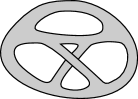
Figure 6: Non-planar-looking closed string graph.

Non-planar graphs

There are two types of non-planar contributions present in the field theory limit of closed string graphs (in gravity amplitudes); non-planar vacuum graphs and planar vacuum graphs where external legs are inside. While the latter may seem to cause no troubles concerning the definition of the loop momentum, the former may appear problematic. They are actually not and are neatly generated by the mechanism of the field theory limit (pinching $a$-cycles), therefore they also come with a uniquely defined loop-momentum. The interested readers can look at the graph in fig. 6 and convince themselves that the graph suggested by the drawing of this Riemann surface can be obtained from a regular “planar-looking” genus 4 surface by pinching a sum of $a$ cycles with $\pm 1$ coefficients.

There are non-orientable open string graphs, and it would be interesting to study the loop momentum of these graphs too.

4 Application to the monodromy relations in open string and gauge theory at loop-level.

Monodromy relations to all loop orders were derived in Tourkine:2016bak in a representation involving loop momentum. Compared to the tree-level case BjerrumBohr:2009rd ; Stieberger:2009hq , the relations do not hold at the level of the amplitude but at the level of the integrand. This stems from the fact that the integrand has both local and global monodromies, and the latter involve phases that depend on the loop momentum. The whole construction is fairly simple and exposed in Tourkine:2016bak so it will not be reviewed too deeply here.

The basic idea is to consider a particular open-string loop-diagram with particles ordered along the boundaries (inner and outer). Using a representation with loop momentum yields directly an integrand that is holomorphic, as we saw above. Therefore, taking one of these particles along a closed contour inside the surface gives, via the residue theorem, that the sum of all individual portion vanishes exactly at the integrand level. Each portion can be rewritten as a properly ordered open string integrand but at the cost of picking up a phase, that depends on the loop momentum when the particle is on a different boundary than the one we started from. The portions of the contour that run along the $a$-cycles (in red in fig. 7) cancel after loop momentum integration (they are related by a simple shift in the loop momentum see Ochirov:2017jby for detailed examples at one-loop).

Figure 7: Two-loop example of field theory limit for open strings and determination of the loop momentum

4.1 Two loops

To be concrete, I provide an example of the field theory limit of two-loop four-gluon amplitude in type I superstring.s

The orientable topologies of the open-string amplitude (no cross-caps) for $\mathcal{N}=4$ Yang-Mills at two loops are obtained from the celebrated two-loop formulae for closed strings of D’Hoker & Phong D'Hoker:2002gw . They read

$$A^{(2)}_{\mathrm{orient}}(1,2,3,4)=s_{12}s_{23}A^{\mathrm{tree}}(1,2,3,4)\int\frac{\prod_{I\leq J}d\Omega_{IJ}}{(\det\,{\,\textrm{Im}\,}\,{\Omega})^{5}}\int_{(\partial\Sigma)^{4}}{\mathcal{Y}}_{S}\exp(\sum_{i,j}k_{i}\cdot k_{j}\mathcal{G}(z_{ij}))\,.$$ (51)

up to a global normalisation factor, and where $A^{\mathrm{tree}}(1,2,3,4)$ is the tree-level four-gluon colour-ordered partial amplitude, while the kinematics invariants are defined by $s_{ij}=-(k_{i}+k_{j})^{2}$. The integration ordered along the boundary $(\partial\Sigma)^{4}\simeq\{\forall i=1\dots 4,z_{i}\in\partial\Sigma,z_{1}<z_{2}<z_{3}<z_{4}\}$ and $\mathcal{Y}_{S}$ is defined by

$$3\mathcal{Y}_{S}=(k_{1}-k_{2})\cdot(k_{3}-k_{4})\,\Delta(z_{1},z_{2})\Delta(z_{3},z_{4})+(13)(24)+(14)(23)\,,$$ (52)

in terms of the differential forms bilinears

$$\Delta(z,w)=\omega_{1}(z)\omega_{2}(w)-\omega_{1}(w)\omega_{2}(z)\,,$$ (53)

For maximally supersymmetric amplitudes in general at two loops in type I and type II, the field theory limit procedure was worked out in Green:2008bf ; Tourkine:2013rda and the numerators are given by the tropical limit of the factor $\mathcal{Y}_{S}$, which equals the kinematic invariant $s_{ij}$ whenever the two legs are on the same $b$-cycle and no sub-triangle is present in the graph, which matches the field theory result of Bern:1997nh (this means that we just have double-box and non-planar double-box graphs).

In terms of the string loop-integrand $I^{(2)}\simeq I^{(2)}(z_{i},\ell_{i})$ of $A^{(2)}_{\mathrm{orient}}$, the monodromy relations of Tourkine:2016bak at two loops read:

$$k_{1}\cdot k_{2}\,I^{(2)}(2134)+k_{1}\cdot(k_{2}+k_{3})I^{(2)}(2314)-\ell_{1}\cdot k_{1}I^{(2)}(234|1|.)-\ell_{2}\cdot k_{1}I^{(2)}(234|.|1)\simeq 0\,.$$ (54)

The two terms on the rightmost part correspond to non-planar amplitudes where the particle $1$ is integrated along the first and second inner disks of the two-loop open string graph, respectively (from left to right in fig. 7). The $\simeq$ symbol means “up to terms that vanish after momentum integration”. These are generated by integrals along the boundary of the cut surface and correspond to loop momentum shifts.

(55)

All other diagrams are suppressed by supersymmetry in the field theory limit, because of the properties of the tropical limit of the integrand given by $\mathcal{Y}_{S}$ that we just described. These graphs are scalar graphs, with their denominator, and with the same numerator $s_{12}=-(k_{1}+k_{2})^{2}$ because $\mathcal{Y}_{s}=s_{34}=s_{12}$ (again see (Tourkine:2013rda, , Tab. 1, p. 41)). Therefore, these graphs are just scalar graphs with constant numerator.

Using the antisymmetry of the three-point vertex Tourkine:2016bak ; Ochirov:2017jby , we can equate the two graphs on the second line up to a sign and reduce the factors in front of the graphs to differences of propagators,

$$\ell_{1}\cdot k_{1}=(\ell_{1}+k_{1})^{2}-\ell_{1}^{2},$$ (56)

$$(\ell_{1}+k_{2})\cdot k_{1}=(\ell_{1}+k_{1}+k_{2})^{2}-(\ell_{1}+k_{2})^{2},$$ (57)

$$(-\ell_{1}+\ell_{2})\cdot k_{1}=(\ell_{1}-\ell_{2})^{2}-(\ell_{1}-\ell_{2}-k_{1})^{2}\,.$$ (58)

In this way, six terms are produced which almost cancel pairwise:

(59)

In this equation, the plain (resp. dashed) lines correspond to a positive (resp. negative sign). Four terms cancel pairwise, while two, the negative contribution of the first graph and the positive one of the last graph, differ by a shift in the loop momentum as:

(60)

Because the relation is exact at fixed loop momentum, this gives a precise definition the terms in the right-hand side. A more graphical explanation of this phenomenon can be found in Ochirov:2017jby . At any rate, after loop momentum integration, these terms cancel, as they should. Note that for more generic amplitudes, the numerators are not simply constants anymore and the field theory limit of the terms on the right-hand side could provide interesting physical quantities. These will be studied elsewhere.

This derivation provides a stronger check than the unitarity cut check that was originally performed in Tourkine:2016bak .

4.2 A relation at three loops

What we have seen so far is that the string representation in terms of loop momentum induces a global definition of the loop momentum. Now we will investigate a new phenomenon related to this that arises at three loops: there are two different vacuum topologies of 1-particle-irreducible graphs, mercedes and ladder, which share the same loop momentum.

After characterizing this effect, we will work out an example of application of the monodromy relations to support further that their connection to the BCJ color-kinematics duality extends to all loops.

Figure 8 displays two representative graphs that follow from the field theory limit of the open string graph on the left-hand side. Both these graphs appear under the same loop-momentum integral in the field theory limit, and provide a natural correspondence between the same loop momentum but in different graphs.

Figure 8: The two graphs on the right-hand side are generated by the field theory limit of the open string graph on the left-hand side. It is an interesting exercise for the reader to work out this example explicitly.

The monodromy relations in string theory at three-loops are obtained by followed the method exposed in Tourkine:2016bak . Circulating the leg $1$ inside a previously planar graph with ordering $1<2<3<4$ as in fig. 8 yields a relation, whose field theory limit is given by

$$k_{1}\cdot k_{2}\,I^{(3)}(2134)+k_{1}\cdot(k_{2}+k_{3})I^{(3)}(2314)\cr-\ell_{1}\cdot k_{1}I^{(3)}(234|1|.|.)-\ell_{2}\cdot k_{1}I^{(3)}(234|.|1|.)-\ell_{3}\cdot k_{1}I^{(3)}(234|.|.|1)\simeq 0\,.$$ (61)

The notations are similar to those of eq. (54). The terms on the second line correspond to non-planar amplitudes where the particle $1$ is integrated along the first, second and third inner disks, respectively, according to the numbering of the $a$ cycles in fig. 8.

Many graphs arise in this integrand relation. They mix different topologies and orderings. The systematics of the propagator cancelation is similar to what happens at two loops. We illustrate this below for a particular subset of these graphs, which will give stronger evidence that a BCJ representation always satisfy the monodromy relation, up to the loop-momentum shifting terms.

The main point is that this sum of graphs can be re-organized into BCJ triplets. For instance, the following four terms appear in the sum in the left-hand side of (61):

$$\includegraphics{3loops.pdf}\\ +\ldots\simeq 0$$ (62)

where $+...$ indicate the rest of the terms of the sum. These graphs represent full integrands: numerators over denominator. They are those of any gauge theory we started with in the open string.

With the momenta are distributed as in fig 8, it is easy to see that the factors in front of the graphs indeed recombine into differences of irreducible propagators which organise themselves as a BCJ identity with shifted momenta of the form:

$$-D\bigg{(}\vbox{\hbox{\includegraphics{./graphs/den-shifted.pdf}}}\bigg{)}\times N\bigg{(}\vbox{\hbox{\includegraphics{./graphs/gr1.pdf}}}\bigg{)}+\\ D\bigg{(}\vbox{\hbox{\includegraphics{./graphs/den-shifted.pdf}}}\bigg{)}\times\bigg{\{}N\bigg{(}\vbox{\hbox{\includegraphics{./graphs/gr2.pdf}}}\bigg{)}+N\bigg{(}\vbox{\hbox{\includegraphics{./graphs/gr3.pdf}}}\bigg{)}\bigg{\}}\,.$$ (63)

Here, $D(\cdot)$ is the scalar denominator corresponding to the graph (non-obvious loop-momentum locations are depicted, $\ell_{2}$ is not affected) and $N(\cdot)$ is the numerator of the corresponding graph. I have used again the antisymmetry of the three-point vertex

$$N\bigg{(}\vbox{\hbox{\includegraphics{./graphs/gr2.pdf}}}\bigg{)}=-N\bigg{(}\vbox{\hbox{\includegraphics{./graphs/gr2sym.pdf}}}\bigg{)}\,.$$ (64)

The three terms above therefore combine into a BCJ triplet involving some loop momentum shifts on top of denominators with one propagator canceled.

We have worked out the specific case that is the most delicate, i.e. the one that involves loop momentum shifts. The other triplet identities are simpler and therefore it is very reasonable to guess that the property persists for all types of tri-valent graphs also including those with internal triangles, bubbles or not – see Ochirov:2017jby for examples at one loop.

Note that an identity that would mix up mercedes and ladder topologies requires to apply the monodromy relations twice or to start from a non-planar amplitude.

To sum up the relations that stem from the monodromy relations in the field theory limit, we schematically denote by the letter $J_{G,e}$ the sum of BCJ triplets for the graph $G$ with one inner edge $e$ contracted. We obtain:

$$\sum_{G,e}\frac{J_{G,e}}{D_{G,e}}\simeq 0$$ (65)

In the generalised double copy construction Bern:2017ucb , these $J$-functions generate higher point vertices that need to be canceled by introducing contact terms. The structure of these objects is still quite poorly understood, in particular how to simplify them as much as possible, and it would be interesting to see if the monodromy relations can provide some formal constraints on these objects, maybe in relation to the loop shifting terms of the right-hand side.

5 Discussion

An integrand in field theory.

In this paper we analyzed some aspects related to the definition of the loop momentum in string and field theory. This formalism was mostly developed to be applied to the monodromy relations, but it would be very interesting to see if the global integrand defined in this way has any nice physical properties.

Furthermore, in standard perturbative field theory there is no particular notion of field theory integrand except in the case of planar amplitudes: this has lead to remarkable constructions such as the all-loop integrand for planar $\mathcal{N}=4$ super-Yang Mills ArkaniHamed:2010kv and the amplituhedron Arkani-Hamed:2013jha . This program was then extended to gravitational theories in Herrmann:2016qea and it would be interesting to see if all these constructions are connected to the general considerations presented in this paper.

The ambitwistor string Mason:2013sva , based on the scattering equation formalism Cachazo:2013iea also provide loop integrands Adamo:2013tsa ; Ohmori:2015sha ; Casali:2014hfa ; Geyer:2015bja ; Geyer:2015jch ; Cachazo:2015aol ; He:2015yua ; He:2015wgf ; Geyer:2016wjx ; Geyer:2018xwu . The bottleneck in pushing this formalism to all loops has so far been the understanding of the geometry of the moduli space and the connection to the zero-modes (loop-momentum) in the path integral. There is no doubts that a better understanding of the loop momentum in string theory should help to fix these issues.

Kawai-Lewellen-Tye

Since they realize splitting of the holomorphic and anti-holomorphic degrees of freedom in string integrands, loop momentum representations should also be linked to the extension of the tree-level Kawai-Lewellen-Tye Kawai:1985xq ; BjerrumBohr:2010hn formulae to loop-level. Recently, Mizera has reformulated in the language of twisted cycles this program Mizera:2017cqs ; Mizera:2017rqa and a deeper understanding of the loop momentum will be necessary to understand these constructions at loop-level where global monodromies arise. Relatedly, it would be very interesting to see if these relations can be extended to amplitudes relations. The theory developped in Mastrolia:2018uzb for field theory integrands, inspired from Mizera:2017cqs , would seem like a natural starting point to study these questions. Relatedly, “generalized elliptic functions” have been introduced in Mafra:2017ioj ; Mafra:2018nla ; Mafra:2018qqe ; Mafra:2018pll and it would be interesting to see if a proper treatment of the loop momentum can help in characterizing the nature of these objects.

Twisted strings and modular invariance

Twisted strings are the tensionful versions of ambitwistor strings. To my knowledge, the first time such a construction was mentioned is in the paper Hwang:1998gs , and in spirit they were present in Gamboa:1989zc ; Gamboa:1989px already. Classically, they are just identical to traditional string theory; but their quantization is modified (different operator ordering) which results in a truncated spectrum. The cleanest way to understrand their scattering amplitudes is at tree-level so far, via the twisted period relations of Mizera:2017rqa .

It is conjectured Siegel:2015axg that the loop level version should also involve only a change in oscillator modes of the string, therefore all we said here about the loop-momentum zero-modes should apply to the twisted string too. However, loop amplitudes have proven difficult to write so far, and a very good hope to guess them would be to generalize the twisted period relations to loop-level. This ties in with the previous paragraph on KLT.

One could even think of using these twisted string loop amplitudes to then take the ambitwistor string limit (tensionless limit of the twisted string, see Siegel:2015axg ; Leite:2016fno ; Huang:2016bdd and Casali:2017zkz ; Casali:2016atr ). But one may doubt that this could produce a sensible answer, mostly because the loop momentum breaks modular invariance DHoker:1988pdl and the saddle point equations of the tensionless limit Gross:1987ar seem to induce a maximum value for the loop momentum, while all values should be allowed and integrated on to give back the original integral without loop momentum. This problem will be studied elsewhere.

Acknowledgements

I would like to thank David Andriot, Enrico Hermann, Alexander Ochirov, Julio Parra-Martinez, Boris Pioline, Amit Sever and Sasha Zhiboedov for useful discussions and comments. This research project has been supported by a Marie Skłodowska-Curie Individual Fellowship of the European Commission’s Horizon 2020 Programme under contract number 749793 NewLoops.

Appendix A Definitions

Here are the conventions that are used in this paper (we follow mostly Kiritsis Kiritsis:2007zza )

$$z=\sigma^{1}+i\sigma^{2},\quad\bar{z}=\sigma^{1}-i\sigma^{2},\quad\frac{\partial}{\partial z}=\frac{1}{2}(\partial_{1}-i\partial_{2}),\quad\frac{\partial}{\partial\bar{z}}=\frac{1}{2}(\partial_{1}+i\partial_{2})$$ (66)

The metric reads $d^{2}s=2g_{z\bar{z}}dzd\bar{z}$, therefore $\sqrt{g}=g_{z\bar{z}}$ such that the volume measure is given by $\int\sqrt{g_{ab}}d^{2}\sigma=\int\sqrt{g}d^{2}z$ which yields

$$2d\sigma_{1}d\sigma_{2}=d^{2}z=idz\wedge d\bar{z}$$ (67)

For the diagonal metric $g_{ab}=\mathrm{diag}(1,1)$ we have $g_{z\bar{z}}=1/2$ which implies that $\delta^{2}(z,\bar{z})=\frac{1}{2\sqrt{g}}\delta(x)\delta(y)=\delta(x)\delta(y)$, as this yields

$$\int\sqrt{g}d^{2}z\delta^{2}(z,\bar{z})=1$$ (68)

We also have

$$\partial_{\bar{z}}\frac{1}{z}=\partial_{z}\frac{1}{\bar{z}}=2\pi\delta^{2}(z,\bar{z})$$ (69)

We will use the language of differential forms (all conventions are spelled out in appendix A), upon which, essentially, c

$$d^{2}z=i{dz\wedge d\bar{z}},\quad\partial=\partial_{z}dz,\quad\bar{\partial}=\partial_{\bar{z}}d\bar{z}\,\quad d=\partial+\bar{\partial}$$ (70)

where $d$ is the standard differential operator, $d^{2}=0$. The $i$ normalisation factor will be important soon. Stokes theorem states that, for $\omega$ a $k$-form and $D$ a $(k+1)$-chain, we have

$$\int_{\partial D}\omega=\int_{D}d\omega$$ (71)

where $\partial D$ is the boundary of $D$.

The prime form is a $(-1/2,0)\otimes(-1/2,0)$ bi-holomorphic form defined on the universal covering of the surface by

$$E(x,y)=\frac{\theta[\nu](\int_{x}^{y}(\omega_{1},...,\omega_{g})|{\Omega})}{h_{\nu}(x)h_{\nu}(y)}\,\in\mathbb{C}\,,$$ (72)

where $h_{\nu}(x)^{2}=\sum_{I}\omega_{I}\partial_{I}\theta[\nu](0|\Omega)$ are half-differentials (section of the square-root of the canonical bundle). It is independent of the spin structure chosen to define it.

The Riemann theta functions are defined by

$$\theta[\nu](\zeta|\Omega)=\sum_{n\in\mathbb{Z}^{g}}e^{i\pi({n}+{\beta})\cdot\Omega({n}+{\beta})}e^{2i\pi({n}+{\beta})\cdot({\zeta}+{\alpha})}$$ (73)

where $\left[\begin{smallmatrix}{\beta}\\ {\alpha}\end{smallmatrix}\right]=\nu\in(\mathbb{Z}/\mathbb{Z}_{2})^{2g}$ is a theta characteristic. They have monodromies that can be found in standard textbooks, which lead to the following monodromies for the prime form DHoker:1988pdl ;

$$E(x,y)\to\exp(-\Omega_{JJ}/2-\int_{x}^{y}\omega_{J})E(x,y)\,.$$ (74)

and trivial signs along $a$ cycles.

References

- (1) J. A. Shapiro, Loop Graph in the Dual Tube Model, Phys. Rev. D5 (1972) 1945–1948.
- (2) E. P. Verlinde and H. L. Verlinde, Chiral Bosonization, Determinants and the String Partition Function, Nucl. Phys. B288 (1987) 357. [,244(1986)].
- (3) E. P. Verlinde and H. L. Verlinde, Multiloop Calculations in Covariant Superstring Theory, Phys.Lett. B192 (1987) 95.
- (4) E. D’Hoker and D. H. Phong, The Geometry of String Perturbation Theory, Rev. Mod. Phys. 60 (1988) 917.
- (5) E. D’Hoker and D. H. Phong, Conformal Scalar Fields and Chiral Splitting on Superriemann Surfaces, Commun. Math. Phys. 125 (1989) 469.
- (6) P. Tourkine and P. Vanhove, Higher-Loop Amplitude Monodromy Relations in String and Gauge Theory, Phys. Rev. Lett. 117 (2016), no. 21 211601, [arXiv:1608.0166].
- (7) E. Plahte, Symmetry Properties of Dual Tree-Graph N-Point Amplitudes, Nuovo Cim. A66 (1970) 713–733.
- (8) N. E. J. Bjerrum-Bohr, P. H. Damgaard, and P. Vanhove, Minimal Basis for Gauge Theory Amplitudes, Phys. Rev. Lett. 103 (2009) 161602, [arXiv:0907.1425].
- (9) S. Stieberger, Open & Closed vs. Pure Open String Disk Amplitudes, arXiv:0907.2211.
- (10) Z. Bern, J. J. M. Carrasco, and H. Johansson, New Relations for Gauge-Theory Amplitudes, Phys. Rev. D78 (2008) 085011, [arXiv:0805.3993].
- (11) Z. Bern, J. J. M. Carrasco, and H. Johansson, Perturbative Quantum Gravity as a Double Copy of Gauge Theory, Phys. Rev. Lett. 105 (2010) 061602, [arXiv:1004.0476].
- (12) Z. Bern, J. J. Carrasco, W.-M. Chen, A. Edison, H. Johansson, J. Parra-Martinez, R. Roiban, and M. Zeng, Ultraviolet Properties of Supergravity at Five Loops, Phys. Rev. D98 (2018), no. 8 086021, [arXiv:1804.0931].
- (13) B. Feng, Y. Jia, and R. Huang, Relations of Loop Partial Amplitudes in Gauge Theory by Unitarity Cut Method, Nucl. Phys. B854 (2012) 243–275, [arXiv:1105.0334].
- (14) B. Feng, R. Huang, and Y. Jia, Gauge Amplitude Identities by On-Shell Recursion Relation in S-Matrix Program, Phys. Lett. B695 (2011) 350–353, [arXiv:1004.3417].
- (15) R. H. Boels and R. S. Isermann, New Relations for Scattering Amplitudes in Yang-Mills Theory at Loop Level, Phys. Rev. D85 (2012) 021701, [arXiv:1109.5888].
- (16) R. H. Boels and R. S. Isermann, Yang-Mills Amplitude Relations at Loop Level from Non-Adjacent Bcfw Shifts, JHEP 03 (2012) 051, [arXiv:1110.4462].
- (17) Y.-J. Du and H. Luo, On General Bcj Relation at One-Loop Level in Yang-Mills Theory, JHEP 01 (2013) 129, [arXiv:1207.4549].
- (18) M. Chiodaroli, M. Gunaydin, H. Johansson, and R. Roiban, Explicit Formulae for Yang-Mills-Einstein Amplitudes from the Double Copy, JHEP 07 (2017) 002, [arXiv:1703.0042].
- (19) M. B. Green, J. H. Schwarz, and E. Witten, Superstring Theory Vol. 2. Cambridge Monographs on Mathematical Physics. Cambridge University Press, 2012.
- (20) D. P. Skliros, E. J. Copeland, and P. M. Saffin, Highly Excited Strings I: Generating Function, Nucl. Phys. B916 (2017) 143–207, [arXiv:1611.0649].
- (21) H. M. Farkas and I. Kra, Riemann surfaces, vol. 71. Springer-Verlag, 1980.
- (22) E. Casali and P. Tourkine, Infrared behaviour of the one-loop scattering equations and supergravity integrands, JHEP 04 (2015) 013, [arXiv:1412.3787].
- (23) M. Bianchi and A. Sagnotti, Open Strings and the Relative Modular Group, Phys. Lett. B231 (1989) 389–396.
- (24) J. Scherk, Zero-Slope Limit of the Dual Resonance Model, Nucl. Phys. B31 (1971) 222–234.
- (25) P. Tourkine, Tropical Amplitudes, Annales Henri Poincare 18 (2017), no. 6 2199–2249, [arXiv:1309.3551].
- (26) J. D. Fay, Theta functions on Riemann surfaces, vol. 352. Springer, 1973.
- (27) E. D’Hoker, M. B. Green, and B. Pioline, Higher Genus Modular Graph Functions, String Invariants, and Their Exact Asymptotics, arXiv:1712.0613.
- (28) P. Dai and W. Siegel, Worldline Green Functions for Arbitrary Feynman Diagrams, Nucl. Phys. B770 (2007) 107–122, [hep-th/0608062].
- (29) S. Hohenegger and S. Stieberger, Monodromy Relations in Higher-Loop String Amplitudes, arXiv:1702.0496.
- (30) A. Ochirov, P. Tourkine, and P. Vanhove, One-Loop Monodromy Relations on Single Cuts, JHEP 10 (2017) 105, [arXiv:1707.0577].
- (31) E. D’Hoker and D. H. Phong, Lectures on Two Loop Superstrings, Conf. Proc. C0208124 (2002) 85–123, [hep-th/0211111]. [,85(2002)].
- (32) M. B. Green, J. G. Russo, and P. Vanhove, Modular Properties of Two-Loop Maximal Supergravity and Connections with String Theory, JHEP 07 (2008) 126, [arXiv:0807.0389].
- (33) Z. Bern, J. S. Rozowsky, and B. Yan, Two Loop Four Gluon Amplitudes in Superyang-Mills, Phys. Lett. B401 (1997) 273–282, [hep-ph/9702424].
- (34) Z. Bern, J. J. M. Carrasco, W.-M. Chen, H. Johansson, R. Roiban, and M. Zeng, Five-loop four-point integrand of supergravity as a generalized double copy, Phys. Rev. D96 (2017), no. 12 126012, [arXiv:1708.0680].
- (35) N. Arkani-Hamed, J. L. Bourjaily, F. Cachazo, S. Caron-Huot, and J. Trnka, The All-Loop Integrand for Scattering Amplitudes in Planar Sym, JHEP 01 (2011) 041, [arXiv:1008.2958].
- (36) N. Arkani-Hamed and J. Trnka, The Amplituhedron, JHEP 10 (2014) 030, [arXiv:1312.2007].
- (37) E. Herrmann and J. Trnka, Gravity On-Shell Diagrams, JHEP 11 (2016) 136, [arXiv:1604.0347].
- (38) L. Mason and D. Skinner, Ambitwistor strings and the scattering equations, JHEP 07 (2014) 048, [arXiv:1311.2564].
- (39) F. Cachazo, S. He, and E. Y. Yuan, Scattering of Massless Particles: Scalars, Gluons and Gravitons, JHEP 1407 (2014) 033, [arXiv:1309.0885].
- (40) T. Adamo, E. Casali, and D. Skinner, Ambitwistor strings and the scattering equations at one loop, JHEP 04 (2014) 104, [arXiv:1312.3828].
- (41) K. Ohmori, Worldsheet Geometries of Ambitwistor String, JHEP 06 (2015) 075, [arXiv:1504.0267].
- (42) Y. Geyer, L. Mason, R. Monteiro, and P. Tourkine, Loop Integrands for Scattering Amplitudes from the Riemann Sphere, Phys. Rev. Lett. 115 (2015), no. 12 121603, [arXiv:1507.0032].
- (43) Y. Geyer, L. Mason, R. Monteiro, and P. Tourkine, One-loop amplitudes on the Riemann sphere, JHEP 03 (2016) 114, [arXiv:1511.0631].
- (44) F. Cachazo, S. He, and E. Y. Yuan, One-Loop Corrections from Higher Dimensional Tree Amplitudes, arXiv:1512.0500.
- (45) S. He and E. Y. Yuan, One-Loop Scattering Equations and Amplitudes from Forward Limit, Phys. Rev. D92 (2015), no. 10 105004, [arXiv:1508.0602].
- (46) S. He, R. Monteiro, and O. SCHLotterer, String-Inspired Bcj Numerators for One-Loop Mhv Amplitudes, JHEP 01 (2016) 171, [arXiv:1507.0628].
- (47) Y. Geyer, L. Mason, R. Monteiro, and P. Tourkine, Two-Loop Scattering Amplitudes from the Riemann Sphere, Phys. Rev. D94 (2016), no. 12 125029, [arXiv:1607.0888].
- (48) Y. Geyer and R. Monteiro, Two-Loop Scattering Amplitudes from Ambitwistor Strings: from Genus Two to the Nodal Riemann Sphere, JHEP 11 (2018) 008, [arXiv:1805.0534].
- (49) H. Kawai, D. C. Lewellen, and S. H. H. Tye, A Relation Between Tree Amplitudes of Closed and Open Strings, Nucl. Phys. B269 (1986) 1–23.
- (50) N. E. J. Bjerrum-Bohr, P. H. Damgaard, T. Sondergaard, and P. Vanhove, The Momentum Kernel of Gauge and Gravity Theories, JHEP 01 (2011) 001, [arXiv:1010.3933].
- (51) S. Mizera, Combinatorics and Topology of Kawai-Lewellen-Tye Relations, arXiv:1706.0852.
- (52) S. Mizera, Scattering Amplitudes from Intersection Theory, arXiv:1711.0046.
- (53) P. Mastrolia and S. Mizera, Feynman Integrals and Intersection Theory, arXiv:1810.0381.
- (54) C. R. Mafra and O. Schlotterer, Double-Copy Structure of One-Loop Open-String Amplitudes, Phys. Rev. Lett. 121 (2018), no. 1 011601, [arXiv:1711.0910].
- (55) C. R. Mafra and O. SCHLotterer, Towards the N-Point One-Loop Superstring Amplitude I: Pure Spinors and Superfield Kinematics, arXiv:1812.1096.
- (56) C. R. Mafra and O. SCHLotterer, Towards the N-Point One-Loop Superstring Amplitude Iii: One-Loop Correlators and Their Double-Copy Structure, arXiv:1812.1097.
- (57) C. R. Mafra and O. SCHLotterer, Towards the N-Point One-Loop Superstring Amplitude Ii: Worldsheet Functions and Their Duality to Kinematics, arXiv:1812.1097.
- (58) W. Siegel, Amplitudes for Left-Handed Strings, arXiv:1512.0256.
- (59) Y.-t. Huang, W. Siegel, and E. Y. Yuan, Factorization of Chiral String Amplitudes, JHEP 09 (2016) 101, [arXiv:1603.0258].
- (60) M. M. Leite and W. Siegel, Chiral Closed Strings: Four Massless States Scattering Amplitude, arXiv:1610.0205.
- (61) E. Casali and P. Tourkine, Winding Modes of Tensionful Ambitwistor Strings, arXiv:1710.0124.
- (62) S. Hwang, R. Marnelius, and P. Saltsidis, A General BRST Approach to String Theories with Zeta Function Regularizations, J. Math. Phys. 40 (1999) 4639–4657, [hep-th/9804003].
- (63) J. Gamboa, C. Ramirez, and M. Ruiz-Altaba, Null Spinning Strings, Nucl. Phys. B338 (1990) 143–187.
- (64) J. Gamboa, C. Ramirez, and M. Ruiz-Altaba, Quantum Null (Super)Strings, Phys. Lett. B225 (1989) 335–339.
- (65) E. Casali, Y. Herfray, and P. Tourkine, The Complex Null String, Galilean Conformal Algebra and Scattering Equations, JHEP 10 (2017) 164, [arXiv:1707.0990].
- (66) E. Casali and P. Tourkine, On the Null Origin of the Ambitwistor String, arXiv:1606.0563.
- (67) D. J. Gross and P. F. Mende, String Theory Beyond the Planck Scale, Nucl. Phys. B303 (1988) 407–454.
- (68) E. Kiritsis, String Theory in a Nutshell. 2007.