An Open Source, Versatile, Affordable Waves in Ice Instrument for Scientific Measurements in the Polar Regions

Abstract

Sea ice is a major feature of the polar environments. Recent changes in the climate and extent of the sea ice, together with increased economic activity and research interest in these regions, are driving factors for new measurements of sea ice dynamics. Waves in ice are important as they participate in the coupling between the open ocean and the ice-covered regions. Measurements are challenging to perform due to remoteness and harsh environmental conditions. While progress has been made in observing wave propagation in sea ice using remote methods, these are still relatively new measurements and would benefit from more in situ data for validation. In this article, we present an open source instrument that was developed for performing such measurements. The versatile design includes an ultra-low power unit, a microcontroller-based logger, a small microcomputer for on-board data processing, and an Iridium modem for satellite communications. Virtually any sensor can be used with this design. In the present case, we use an Inertial Motion Unit to record wave motion. High quality results were obtained, which opens new possibilities for in situ measurements in the polar regions. Our instrument can be easily customized to fit many in situ measurement tasks, and we hope that our work will provide a framework for future developments of a variety of such open source instruments.

Keywords Waves in ice  $\cdot$ Open Source instrument  $\cdot$ In situ measurements

1 Measurements of waves in ice

The interaction between surface waves and sea ice involves many complex physical phenomena such as viscous damping (Weber,, 1987; Rabault and others,, 2017), wave diffraction (Squire and others,, 1995), and nonlinear effects in the ice (Liu and Mollo-Christensen,, 1988). Therefore, it is complex and still an area of ongoing research (Rabault,, 2018; Squire,, 2018). Better understanding and modeling of wave propagation in sea ice can allow for the improvement of ocean models to be used for climate, weather and sea state predictions (Christensen and Broström,, 2008), the estimation of ice thickness (Wadhams and Doble,, 2009), and the analysis of pollution dispersion in the Arctic environment (Pfirman and others,, 1995; Rigor and Colony,, 1997). More generally, all these aspects must be better understood to allow safe, environment-friendly operations in the Arctic. Therefore, there is considerable interest in measuring sea ice dynamics.

While the use of Synthetic Aperture Radar (SAR) images from satellites to obtain spectral wave information has made significant progress lately, they are still not standard measurements. Indeed, they require the satellite to be in a particular sampling mode (wide swath), as well as accurate prediction of the azimuth cutoff wavelength. This is vital for accurate determination of the wave energy, and is made complicated by the presence of sea ice (Ardhuin and others,, 2017; Stopa and others,, 2018). Therefore, in situ measurements are still a key method for measurements of waves in ice. In addition, as remote sensing and satellite-based measurements are still relatively new, they still benefit greatly from validation with in situ observations. Such in situ measurements are usually performed using tiltmeters, accelerometers, and more recently further refinements around those devices in the form of Inertial Motion Units (IMUs), which combine several physical measurements (acceleration, angular rates, and magnetic field) together with signal processing capabilities in a single device (Wadhams and Squire,, 1980; Wadhams,, 1979; Liu and others,, 1991; Doble and others,, 2006; Doble and Bidlot,, 2013; Doble and others,, 2017; Marchenko and others,, 2019). Unfortunately, the harsh environment sets demanding requirements for scientific observations in the Arctic. Several commercial solutions are available (companies selling instruments operating in the arctic include, e.g., Sea Bird Scientific Co., Campbell Scientific Co., Aanderaa Data Instruments A.S.), but these usually have a high cost and reduced flexibility, being closed-source black boxes. This is especially problematic as there is a broad consensus in the community that more observations are needed to further develop waves in ice models. In particular, modeling and parametrization of wave attenuation by sea ice remains a topic of active research (Wang and Shen,, 2010a, b; Zhao and Shen,, 2015; Sutherland and others,, 2019; Rabault and others,, 2019; Marchenko and others,, 2019). In addition, the strong spatial inhomogeneity of the ice has proven to be important for the evaluation of wave damping and ice melting, and studying the effect of such spatial variations in more detail will require many instruments to be deployed simultaneously on large-scale field-measurements campaigns, which in turns strengthens the need for affordable, customizable instruments (Horvat and others,, 2016; Horvat and Tziperman,, 2015; Roach and others,, 2018; Hwang and others,, 2017). Fortunately, off-the shelf sensors and open source electronics are now sufficiently documented and easy to use as to become a credible alternative to traditional solutions. Therefore, they may offer a solution for gathering the large amounts of data that the community needs, at a reduced cost.

In a recent work (Rabault and others,, 2017), a simple open-source instrument for the measurement and logging of waves in ice was developed. This design was further improved and iterated, by adding on-board processing and satellite communication capabilities. As a consequence, the new instrument has become a powerful solution for performing in situ measurements of complex physical processes such as waves in ice. In this article, we provide a detailed technical description of this new instrument, a brief overview of the data collected which confirms proper functionality, a cross-validation against both data collected using another kind of instrument and a wave model, and we discuss implications for the communities performing in situ measurements in the polar regions. We believe that releasing our design as open source material may help create a scientific community sharing the design of their instruments, therefore making the study of the Arctic much more cost effective and enabling far more data to be collected.

2 Technical solution used

In this section, we present a technical description of the design and performance of the waves in ice instrument. All the code and the files for the Printed Circuit Board (PCB) are released as Open Source material (see Appendix A), so that our design is fully reproducible. Moreover, the design is highly modular, and therefore it would be easy to add sensors to the logger and to measure and transmit additional information, such as wind speed, temperature, humidity, irradiance, or any other relevant physical quantity that could be required. We choose to design our instrument around affordable, easily available and well documented hardware such as Arduinos and Raspberry Pis, and we prefer solutions that are slightly non-optimal but easy to build, rather than more involved designs which would require sophisticated assembly.

2.1 Hardware

The technical solution used in the present work is a further development of what was presented in Rabault and others, (2017). At the core of the instrument lies a GPS and a high-accuracy, thermally calibrated IMU. The IMU chosen is the VN100, produced by Vectornav Co. It includes a 3-axis accelerometer, 3-axis gyroscope, 3-axis magnetometer, pressure sensor, temperature sensor, and a 32 bit processor for running an on-board extended Kalman filter. This IMU has been tested and used in a series of previous works (Rabault and others,, 2016, 2017; Sutherland and Rabault,, 2016; Marchenko and others,, 2017), which allowed us to both confirm the quality of the data acquired by the IMU and provide valuable information about wave propagation and attenuation in landfast ice and some grease ice layers. Using the on-board Kalman filter together with low-pass filtering of the signal, wave motion can be accurately measured (Sutherland and others,, 2017).

The newer version of the instrument, which was tested on landfast ice in Tempelfjorden, Svalbard in March 2018 and deployed during the Physical Processes cruise of the Nansen legacy research project in September 2018 (Reigstad and others,, 2017), has extended capabilities compared with the simple logger presented in Rabault and others, (2017). Namely, it integrates a Raspberry Pi microcomputer which can process the data in situ and generate compressed spectra from the data recorded, together with an Iridium modem which enables satellite communications. Moreover, a low-power unit is added to allow for efficient energy use which, together with the addition of a solar panel, allows for long term operation. In the following, the older instruments without in situ processing and satellite communications will be referred to as “waves in ice loggers”, as they basically perform regular logging and timestamping of the signal from the VN100, while the new instruments will be referred to as “waves in ice instruments”.

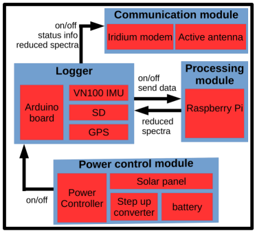
Figure 1: The general architecture of the instrument. Using a modular design, where different components are added on a master Printed Circuit Board (PCB) on top of an Arduino board allows a high level of flexibility for future use.

More specifically, the waves in ice instrument is composed of 4 main modules, as indicated in Fig. 1:

• A power control module - composed of a low power microcontroller, a LiFePO4 battery cell, a solar panel, and a step-up converter - takes care of power management. LiFePO4 battery technology is chosen owing to the robustness of the cells, and their ability to withstand low temperatures. The step-up converter generates the 5V supply needed by the electronics, from the voltage of a single battery cell. The microcontroller takes care of implementing the logic of the power control. Namely, it controls the charging of the battery by coupling the solar panel, and when the logger itself should be waked up. This module is optimized for low energy use, being the only one that is always powered on.

• The logger itself, which records the wave motion, is composed of an Arduino board, the VN100 IMU, a GPS, and a SD card for storing the data. It is very similar to the waves in ice logger which was presented in Rabault and others, (2017). The logger is activated by the power controller approximately every 5 hours, and performs measurements of waves in ice for 25 minutes. The use of an Arduino board means that other sensors could be easily interfaced in both hardware and software, and added to the logics of the instrument. The sleeping time, which decides the duration between consecutive measurements, can be modified in the software and it is discussed further later in the text.

• The processing module, composed of a Raspberry Pi microcomputer running a stripped-down version of Linux, takes care of analyzing the data generated by the logger, and generating the compressed spectra that are sent through Iridium. It communicates with the Arduino board for both receiving the waves data, and sending the compressed results.

• The communication module, which comprises an Iridium modem and the active antenna, allows transmission of data through satellite. The modem is driven by the Arduino board. The Short Burst Messages (SBM) protocol, allowing messages of 340 bytes to be sent by the modem, and 270 bytes to be received from the satellite, is used for communications as it is both cost effective and sufficient for sending compressed data.

All the components are integrated on a central PCB, which connects all the modules together, see Fig 2. This makes the instrument easy to produce and assemble. The whole instrument is packaged into a single Pelican Case with the solar panel mounted on the top, which makes it rugged, compact and convenient to use in fieldwork (dimensions are $34\times 30\times 15$ cm). This packaging of the instrument was chosen as our aim is primarily to measure waves in ice, and are intended to be deployed on ice floes rather than floating on water. Of course, the electronics, sensor and battery could be packaged in another container if the aim would be to perform measurements while floating in the ocean, in which case the hydrodynamic response of the instrument would play a role and the hull of the instrument should be carefully designed. In releasing our design as open source allows for groups with different needs to easily adapt our solution to their requirements. In its present form, the complete design weights about 4.5 kg and all the antennas are mounted inside the case. This means that the instrument is self-contained, robust and easy to deploy. The PCB is designed in KiCAD, an open source electronics CAD software and can be directly produced at a low cost. Therefore, the typical total cost of the complete instrument is around 2000 US$, where the IMU itself represents around 1100 US$ of the total cost. One instrument can be built in around 4 to 6 hours of work.

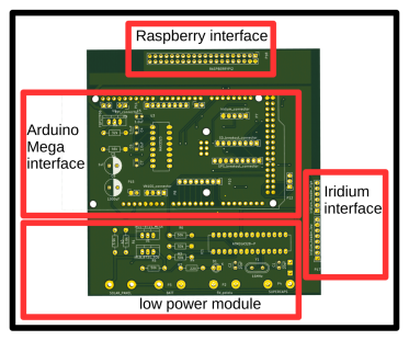
Figure 2: The general layout of the main PCB on which all components are mounted. The full CAD files are released as open source material, see Appendix A.

2.2 Software and in situ data processing

This section presents the software workflow for workflow the instrument. It should be noted that this workflow can be easily customized in software to change the activity pattern or integrate additional measurements:

• At the beginning of each measurement cycle, the low-power unit of the instrument wakes up the logger.

• The logger measures waves in ice using the IMU and records GPS information during 25 minutes.

• When the measurements are finished, a status message is sent through Iridium. This contains information such as the logger GPS position, the battery level, and some technical information about the logger health.

• Following transmission of the status information, the Raspberry Pi (RPi) is triggered to wake up. It receives a copy of the data that has just been recorded, processes the data so as to produce compressed spectra, transmits the data back to the logger, and shuts itself down. The RPi is only awake for a few minutes.

• Following shutdown of the RPi, the logger transmits the compressed spectra through Iridium.

• Finally, the logger is shut down and only the low-power unit is kept operating. The instrument goes into ultra low power mode for a pre-programmed time interval of around 5 hours, which can be modified in software as previously mentioned.

The code for the low power unit and the logger is written in C++, while the signal processing on the RPi is in Python. The Iridium transmission cost is kept low as only compressed spectra and some status information are transmitted. The typical Iridium cost is about 3 $ a day. While it would be possible to send more data by transmitting a succession of Short Bust Data (SBD) messages (according to the data sheet of the Iridium modem, it should be possible to transmit one SBD packet each 10 seconds), we preferred to avoid such a solution as this would increase the cost per day (though this is not the main motivation, as the communication costs remain limited compared with the price of the instrument), energy consumption (transmitting information by satellite is quite energy demanding), and most importantly this would require us to split the data between several SBD packets, which reduces reliability of the whole system. Indeed, this means that if just one packet as part of a multi-packet message gets lost, the whole data is potentially corrupted and useless. Regarding the capabilities of the Iridium modem we use, we also note that it allows for bi-directional communications with the instrument. This means that further developments in the software would allow for remotely controlling the behavior of the instrument, such as the time interval between measurements. This could allow different groups to adapt our instrument to their needs by performing minor changes into the software, which is much less time consuming than developing a new design from scratch. Such updates could also be used to modify, for example, the frequency at which measurements are performed, so that even intermittent phenomena could be captured if they are expected to play an important role (Doble and others,, 2017; Collins and others,, 2015).

As a consequence of the limited amount of data that can be transmitted through Iridium using the SBD packets, the in situ data processing and compression are important parts of the design. All of the onboard data processing is performed based on data sampled at 10 Hz. This includes the calculating of auto- and co-spectra and any integrated spectral parameters we wish to send by Iridium. In addition, the first five Fourier coefficients, i.e. the 1-D energy spectrum and the four directional coefficients, are sent via Iridium at a reduced frequency resolution in order to meet our requirements for data transmission. Details of the onboard data processing can be found in the subsequent paragraphs.

The vertical acceleration ($a_{z}$) and the two orthogonal components of the buoy slope (i.e. pitch and roll) are recorded internally at 10 Hz on the North, East and Down reference frame as calculated by the onboard Kalman filter (running internally at 800Hz together with the raw data acquisition). To calculate the vertical displacement $\eta$ the vertical acceleration is integrated twice with respect to time in the frequency domain using the same method as Kohout and others, (2015). This is done by calculating the Fourier transform and using the frequency response weights of $1/\omega^{2}$ and a half-cosine taper for the lower frequencies to prevent an abrupt cut-off (Tucker and Pitt,, 2001), i.e.

$$\eta(t)=\mathrm{IFFT}\left[H(f)\mathrm{FFT}(a_{z})\right],$$ (1)

where $\mathrm{FFT}$ and $\mathrm{IFFT}$ denote the Fourier and Inverse Fourier transforms respectively and $H(f)$ is the half-cosine taper function,

$$H(f)=\begin{cases}0,&0<f<f_{1}\\ \frac{1}{2}\left[1-\cos{\left(\pi\frac{f-f_{1}}{f_{2}-f_{1}}\right)\left(\frac{-1}{2\pi f^{2}}\right)}\right],&f_{1}\leq f\leq f_{2}\\ \frac{-1}{2\pi f^{2}},&f_{2}<f<f_{c},\end{cases}$$ (2)

where $f$ is the frequency, $f_{c}$ is the Nyquist frequency, and $f_{1}$ and $f_{2}$ are the corner frequencies for the half-cosine taper. We use the same corner frequencies as Kohout and others, (2015) of $f_{1}=0.02\mathrm{Hz}$ and $f_{2}=0.03\mathrm{Hz}$, which are suitable for waves of period in the range of 4 to 20 s. The time series of the vertical displacement is then the real part of the inverse Fourier transform.

The spectra and co-spectra of these time series can be used to provide the directional distribution, which is usually written as (Kuik and others,, 1988)

$$E(f,\theta)=S(f)D(f,\theta),$$ (3)

where $S(f)$ is the 1-D power spectral density (PSD, also referred to as $PSD_{\eta}$ in the following), calculated from the heave, and $D(f,\theta)$ is the normalized directional distribution which has the property

$$\int_{-\pi}^{\pi}D(f,\theta)d\theta=1.$$ (4)

While several methods exist to calculate $D(f,\theta)$ (Kuik and others,, 1988; Sutherland and others,, 2017) they are predominantly based on the following four Fourier coefficients (Longuet-Higgins,, 1963):

$$a_{1}(f) =\int_{-\pi}^{\pi}\cos\left(\theta\right)D(f,\theta)d\theta=\frac{Q_{zx}(f)}{k(f)C_{zz}(f)}$$ (5)

$$b_{1}(f) =\int_{-\pi}^{\pi}\sin\left(\theta\right)D(f,\theta)d\theta=\frac{Q_{zy}(f)}{k(f)C_{zz}(f)}$$ (6)

$$a_{2}(f) =\int_{-\pi}^{\pi}\cos\left(2\theta\right)D(f,\theta)d\theta=\frac{C_{xx}(f)-C_{yy}}{k^{2}(f)C_{zz}(f)}$$ (7)

$$b_{2}(f) =\int_{-\pi}^{\pi}\sin\left(2\theta\right)D(f,\theta)d\theta=\frac{2C_{xy}(f)}{k^{2}(f)C_{zz}(f)},$$ (8)

where $C$ represented the auto- and co-spectra and $Q$ the quadspectra, with $x$, $y$ and $z$ denoting the pitch, roll and heave respectively. Here $k(f)$ is the wavenumber, which can be obtained from the known dispersion relation or estimated from the autospectra as:

$$k(f)=\left(\frac{C_{xx}(f)+C_{yy}(f)}{C_{zz}(f)}\right)^{1/2}.$$ (9)

While the software infrastructure necessary for obtaining directional wave information is already in place, we will not discuss this issue further here. Indeed, more work needs to be done on the current instrument to make sure that the compass of the IMU is isolated from magnetic disturbances induced by the battery and electronics.

Equation (9) is sometimes used as a quality control flag (Tucker and Pitt,, 2001) when the dispersion relation is known, e.g. with the open water dispersion relation $k_{0}=\omega^{2}/g$ where $\omega$ is the angular frequency ($2\pi f$) and $g$ is the acceleration due to gravity. For waves in ice, there are several motivations here for using the open water dispersion relation, rather than a dispersion relation taking into account the effect of the ice. First, it would be challenging to perform a direct estimation of the ice thickness from the data recorded, and such estimation would probably be noisy and brittle, and therefore unsuited for an autonomous instrument operating on its own. Moreover, it seems relatively well established that the dispersion relation in thin broken ice representative of the marginal ice zone (MIZ) is, for practical matters, well described by the open water dispersion relation as was reported in several studies (Sutherland and Rabault,, 2016; Marchenko and others,, 2017; Sutherland and Dumont,, 2018). This is due to the existence of many cracks and regions of open water between the floes that prevent the transmission of flexural stresses, while at the same time the added mass effect of the ice is negligible for the typical range of frequencies encountered. When sending data via Iridium we will use this ratio,

$$R(f)=\left(\frac{C_{xx}(f)+C_{yy}(f)}{C_{zz}(f)}\right)^{1/2}\frac{g}{\omega^{2}}.$$ (10)

The spectra are calculated using the Welch method (Earle,, 1996) and 12000 samples (20 minutes at 10 Hz sampling), using a hanning window on 1024 sample segments and a 50 % overlap. The Fourier coefficients are then downsampled into 25 logarithmically equally spaced bins between 0.05 Hz and 0.25 Hz. This type of sampling gives greater resolution at low frequencies (a minimum resolution of 0.0035 Hz near 0.05 Hz) and less at higher frequencies (a maximum resolution of 0.0162 Hz near 0.25 Hz). Therefore this downsampling strategy allows for greater resolution at low frequencies where most of the wave energy in ice is expected to be prevalent.

All the parameters of this processing algorithm are chosen following previous work on in situ measurements of waves in ice (Kohout and others,, 2014, 2015), and can be modified in the software by the user if one needs to adapt to specific conditions. Of course, modifying some of those parameters, such as the frequency cutoffs or the frequency range exported, may change the amount of data generated and may require some additional adaptations of the compression method. In addition, introducing variability in the configuration of the instruments may be a source of possible mistakes, and it may be worth in this case to consider adding some basic information about the frequency vector of the data transmitted in the SBD messages, to allow cross-checking.

Each Iridium message containing the spectral parameters consists of 340 bytes (as previously mentioned, this is imposed because of how the Iridium SBD protocol works). This includes estimates of the significant wave height and zero-upcrossing, calculated both from the time series as well as from the spectral moments, as well as the reduced six spectra: $S(f)$, $a_{1}(f)$, $b_{1}(f)$, $a_{2}(f)$, $b_{2}(f)$ and $R(f)$. In order to reduce the number of bytes sent via Iridium the maximum absolute value ($\mathrm{max}_{i}$) for each array is sent as a 32-bit float, and the array is sent as a signed 16-bit integer between $-\mathrm{max}_{i}$ and $\mathrm{max}_{i}$.

The significant wave height and zero-upcrossing periods are calculated from both the full time series and the full spectrum. Both temporal and spectral methods are used for redundancy checks to compare with the reduced spectrum also sent via Iridium. The frequency integration bounds used cover the same frequency range as transmitted by Iridium. The significant wave height can be calculated from the time series as $H_{St}=4\mathrm{std}(\eta)$ where $\eta$ is the elevation time series. The significant wave height (SWH) can also be calculated from the spectral moment as $H_{S0}=4\sqrt{m_{0}}$ where the $n_{th}$ spectral moment is defined as

$$m_{n}=\int_{0.05}^{0.25}f^{n}S(f)df,$$ (11)

where we use the same frequency limits as the ones of the transmitted spectrum.

The use of integration limits that are more restrained than the complete extent of the spectra means that $H_{S0}$ is a filtered version of $H_{St}$ (if the whole spectra were used, then $H_{St}$ and $H_{S0}$ would be equal). Therefore, comparing those two values can be seen as a simple self-consistency check of the methodology used.

In the following, we will use the abbreviation “SWH” to signify significant wave height in a general way for example in axis labels, while more detailed captions will refer to the methodology used by writing either $H_{S0}$ or $H_{St}$.

The typical wave period can also be evaluated in several ways. The zero-upcrossing period can be calculated from the time series by calculating the mean time between successive times where $\eta$ goes from positive to negative, in which case it is referred to as $T_{Z0}$. The zero-upcrossing period can also be estimated using spectral moments, i.e. $T_{z}=\sqrt{m_{2}/m_{0}}$. In addition, we will refer in the following to the average crest period $T_{c}=\sqrt{m_{2}/m_{4}}$, and the spectral peak period $T_{p}$, which is defined as the frequency for which the wave spectrum reaches its maximum. Here also, using different methods to compute the same underlying physical quantity can be viewed as a simple cross-checking of the data. In the following, we refer to those quantities in general as the wave period (’WP’ in abbreviation), while specific curves will be labeled by the exact methodology used. A summary of all the variables sent via Iridium, and the precision of each, can be found in Table 1.

Variable	Machine precision
Significant wave height $H_{St}$ (from time series)	32-bit floating point
Zero-upcrossing period $T_{Z0}$ (from time series)	32-bit floating point
Significant wave height $H_{S0}$ (from spectral moment)	32-bit floating point
Zero-upcrossing period $T_{z}$ (from spectral moments)	32-bit floating point
magnitude of $S(f)$	32-bit floating point
magnitude of $a_{1}(f)$	32-bit floating point
magnitude of $b_{1}(f)$	32-bit floating point
magnitude of $a_{2}(f)$	32-bit floating point
magnitude of $b_{2}(f)$	32-bit floating point
$S(f)$ at 25 frequencies	25 $\times$ 16-bit signed integer
$a_{1}(f)$ at 25 frequencies	25 $\times$ 16-bit signed integer
$b_{1}(f)$ at 25 frequencies	25 $\times$ 16-bit signed integer
$a_{2}(f)$ at 25 frequencies	25 $\times$ 16-bit signed integer
$b_{2}(f)$ at 25 frequencies	25 $\times$ 16-bit signed integer
$R(f)$ at 25 frequencies	25 $\times$ 16-bit signed integer

Table 1: Transmitted data via Iridium. A total of 340 bytes is sent per Iridium message.

After receiving the compressed data via Iridium, similar data decompression is implemented and applied to decrypt the messages transmitted. Moreover, a step of de-noising is applied to the transmitted spectra on the receiver side. Applying denoising on the receiver side allows to switch it on and off, to perform quality checks if necessary. Namely, the IMU has a stable noise characteristic which translates into a reproducible background noise on the spectra as illustrated in Fig. 3. In all the following, denoising will only be discussed and applied to the 1-D PSD (i.e., $S(f)$), but this approach could be generalized to the other Fourier coefficients that are being transmitted.

While some information about spectral noise levels are available in the datasheet of the IMU, this is often difficult to translate into a real-world estimate of the noise background due to the internal Kalman filtering, and processing applied on the signal. Therefore, the noise level as a function of frequency $n(f)$ is obtained by fitting a theoretical shape of the form $n(f)=(9.81\times 10^{-3}C)^{2}(2\pi f)^{-4}$ to a record obtained on still ground, where $C$ has unit mg$/\sqrt{\mathrm{Hz}}$ (where we mean “milli g” by mg, and the renormalization numerical constant of value $9.81\times 10^{-3}$ has the unit of ms^-2/mg to enforce dimensionality) and characterizes the noise level. This specific noise shape is chosen as it describes the effect of a uniform spectral noise density on the acceleration measurements when converted into the elevation wave spectra, taking into account the double integration that takes place during the processing. As visible in Fig. 3, this theoretical noise shape is well verified. We find experimentally that $C=0.24$mg$/\sqrt{\mathrm{Hz}}$ describes the obtained noised satisfactorily, which compares reasonably well with the product specification of the VN100 (which states that the spectral noise density should be $0.14$ mg/${\sqrt{\mathrm{Hz}}}$, Vectornav Corporation, (2018)), taking into account that the datasheet value may be an optimistic estimate obtained in the laboratory.

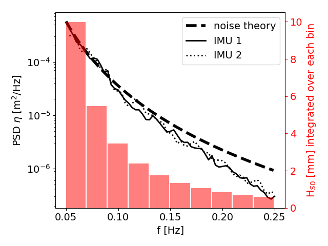
Figure 3: Illustration of the stable noise level of the IMU after processing with the Welch algorithm. The IMUs 1 and 2 are two different VN100 IMUs that were used for tests on still ground. The noise level is consistent across both IMUs, which can be used to denoise afterhand the transmitted spectra. The noise theory is obtained by fitting a theoretical noise shape to the data on the high frequency part of the spectra, where the effect of noise is most important due to the double integration performed to compute the wave elevation. Finally, the histogram presents $H_{S0}$ obtained by integrating over the width of each of the bins, and provides an estimate of the effective noise level of the instruments at each frequency.

In practice, the effect of noise can be neglected for waves larger than around 10 mm at a frequency of 0.15Hz. However, in the case when small waves (i.e. typically under 5 mm at 0.15Hz) are observed, correcting for this background noise improves the quality of the measurements especially for the lowest frequency where the noise introduced by the double integration of the vertical acceleration is largest. More specifically, we consider that the wave signal $s(t)$ and the IMU noise $n(t)$ are uncorrelated, and we want to compute the power spectral density of the combined output $w(t)=s(t)+n(t)$. Remembering that the power spectral density is the Fourier transform of the auto-correlation function $\Gamma$, we mean to calculate:

$$\Gamma_{w,w}(\tau)=\mathbb{E}\left[(s(t)+n(t))(s(t+\tau)+n(t+\tau))\right].$$ (12)

Applying the distributivity of the expected value operator and using the condition that the signals $s$ and $n$ are uncorrelated, the cross-terms disappear leading to $\Gamma_{w,w}(\tau)=\Gamma_{s,s}(\tau)+\Gamma_{n,n}(\tau)$, therefore $PSD(w)=PSD(s)+PSD(n)$. This means that the stable sensor noise level can be subtracted from the power spectral density of the transmitted spectra to reduce noise. In the following, this processing will be applied to the wave elevation spectra.

3 Deployment on the ice

3.1 Deployment on landfast ice in Tempelfjorden, Svalbard and validation of the on-board algorithms

In this subsection, we present a cross-validation of the algorithms and methodology used for the on-board processing and Iridium data compression by comparing results obtained from the raw data recorded by a waves in ice logger and processed using the methodology previously presented in Rabault and others, (2017), against the results obtained from a waves in ice instrument, which were transmitted over Iridium.

The data were obtained during a deployment in landfast ice in Tempelfjord, Svalbard performed in March 2018. The ice conditions were similar to what were encountered in an earlier deployment in 2015 (Sutherland and Rabault,, 2016), see Fig 4. A waves in ice logger and a waves in ice instrument were deployed side-by-side on the frozen fjord, around 500 meters from the ice edge. Both performed measurements from March 21st to March 27th. Surface waves were observed between the evening on March 22nd and early afternoon on March 23rd. As the deployment took place on landfast ice in the inner part of a fjord, the waves were small (the peak significant wave height was about 2.5 cm), but nonetheless could be reliably measured by our instruments.

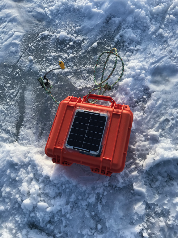
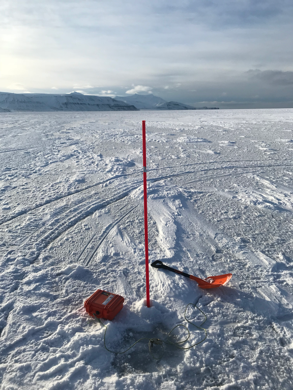
Figure 4: Illustration of the deployment of a waves in ice instrument on landfast ice in Tempelfjorden, Svalbard (left), and waves in ice logger deployed on its side (right). The shovel gives an idea of the size of the instrument boxes.

The spectrograms obtained by both instruments are presented in Fig. 5. Obviously, the resolution in time is much higher in the case of the logger (which records data continuously) than with the iridium-enabled instrument which transmits data only around each 3 hours (as this was a test run over a shorter amount of time, the wakeup frequency was increased compared to the standard value of 5 hours). The resolution in frequency is also reduced, due to the integration and down-sampling of the spectra, which has the effect of reducing the resolution of the individual spectra. However, both the distribution and typical value of the power spectral density are satisfactorily reproduced by the under-sampled spectrogram (this will also be shown in more details in the next paragraph). In addition, we also want to stress that, as was mentioned previously, the wakeup and transmission frequency could easily be increased if deemed necessary for a different task, and it would be even possible to control this parameter through the 2-ways iridium link by developing additional software.

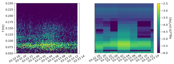
Figure 5: Comparison between the spectrogram produced from analyzing the data logged continuously by a waves in ice logger (left), and the spectra produced in situ and transmitted using Iridium by a waves in ice instrument (right). The data were generated during a deployment on landfast ice in Tempelfjorden, Svalbard in March 2018. While the frequency and time resolutions are, obviously, lesser in the second case, both the energy level and frequency distribution of the wave signal are very similar in both cases.

A more detailed comparison between the results obtained by the waves in ice instrument and the waves in ice logger is presented in Fig. 6. As visible in Fig. 6, the spectra agree well, which provides a more detailed illustration of the results presented in Fig. 5. In this figure, and in all the following when error bars will be presented either for wave spectra or for reports of significant wave height, a 3-$\sigma$ confidence interval is used. Confidence intervals are calculated from the Chi-squared distribution, following the methodology presented in Young, (1986, 1995); Specialist Committee on Stability in Waves of the 28th ITTC, (2017), where the number of degrees of freedom is calculated from the number of overlapping segments used in the Welch method (Kohout and others,, 2015).

Therefore, the agreement observed in this subsection cross-validates the in situ, on board data processing against the data processing our group has been using in the past, as well as the data compression and decompression algorithms used to transmit the reduced spectra over Iridium. This is especially important as there are many fully autonomous steps involved in the on-board data processing, data compression and transmission, and therefore the results of this section offer a cross-validation suggesting that the algorithms and implementations used are indeed functioning correctly in the autonomous instrument when no human expertise or inspection is available.

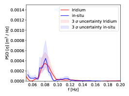
(a) 2018-03-22 21:00

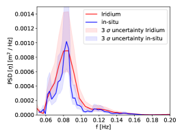
(b) 2018-03-23 02:00

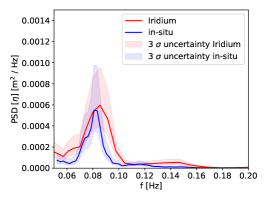
(c) 2018-03-23 18:00

Figure 6: Comparison between the wave spectra obtained from the waves in ice instrument and the waves in ice logger before, during, and after the peak wave activity recorded. This provides a cross-validation of the processing algorithm and of the data compression methodology used in the waves in ice instrument.

3.2 Deployment on a large ice floe in the Marginal Ice Zone in the Barents sea, and comparison with the data obtained from nearby pressure sensors

In this subsection, we compare the results obtained using a waves in ice logger with those of a nearby pressure sensor mounted under the ice during a field campaign on a large ice floe in the Barents sea during May 2016. Both datasets have been presented previously in the literature (Marchenko and others,, 2017), and here we simply offer a more detailed assessment of the agreement between the two methodologies as a way to validate our instrument. As the waves in ice logger has been cross-validated against the waves in ice instrument in the previous subsection, this constitutes a validation of both of them against a different measurement technique.

In all of the following, the data from the IMU loggers will be analyzed following the same methodology as in the previous sections, while the analysis of the pressure records will follow the methodology presented in (Marchenko and others,, 2013, 2017). The pressure measurements were performed using a Sea Bird SBE39 plus equipped with a laboratory-calibrated pressure probe, measuring at a sampling rate of 2.0Hz. The relation in the spectral domain between the pressure and elevation spectra can be written as (Marchenko and others,, 2013, 2017):

$$S_{p}(z,f)=S_{\eta}(f)\left[P(k,z)\rho_{w}g\right]^{2},$$ (13)

with $P(k,z)$ a transfer function defined as:

$$P(k,z)=\frac{\cosh(k(z+H))}{\cosh(kH)}-1,$$ (14)

where $S_{p}(z,f)$ is the spectrum of the pressure fluctuations at depth $z$ (in our case, $z=11$m), $\rho_{w}$ is the density of water, $g$ the acceleration of gravity, $S_{\eta}(f)$ the wave elevation spectrum, $k$ the wavenumber, and $H=160$m the water depth. As measured in Marchenko and others, (2017), the dispersion relation is not affected by the relatively thin ice floe in the frequency band where wave motion is present, and therefore we use the dispersion relation for open water of intermediate depth, $\omega^{2}=gk\tanh(kH)$, with $\omega=2\pi f$ the angular frequency.

Following this methodology, a typical peak significant wave height of about $12$ cm is obtained with both the IMU-based logger and the pressure sensor, as visible in Fig. 7 and already reported in Marchenko and others, (2017). In addition, both the evolution in time of the significant wave height and sample spectra taken at specific times (presented in Fig. 8) demonstrate good agreement between the two measurement techniques. Although a slight difference (at the limit of statistical significance) can be observed between the waves in ice instrument and the pressure sensor for frequencies of around 0.7 Hz, we believe that this can come from either oscillations of the pressure sensor (the pressure sensor is attached under the ice on a weighted rope, and therefore small oscillations of the sensor may be introduced by the waves and ice motions), and / or from the fact that both instruments were deployed a few meters away from each other, therefore, the response of the ice floe to the waves may be slightly different at both locations. In addition, pressure sensors may also measure pressure fluctuations that are appearing due to local hydrodynamic processes in the water, for example originating from waves / current interaction or eddy processes, that may add some energy in specific frequency ranges. Therefore, we consider that the data provided in this section are in good enough agreement that they successfully validate our results against a different instrument and measurement technique.

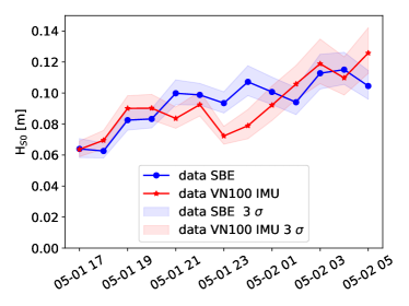
Figure 7: Comparison between the significant wave height computed from the IMU-based and pressure-based instruments, as a function of time. The colored area presents the confidence intervals at 3-$\sigma$. Both the general trend and the typical value of the significant wave height are in good agreement between the two methodologies.

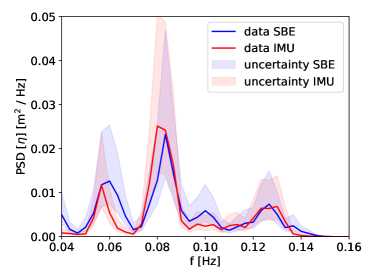
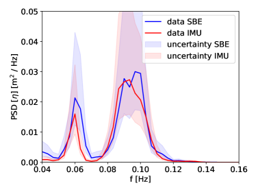
Figure 8: Comparison between the frequency spectra for the wave elevation computed based on the pressure (SBE) and acceleration (IMU) data. The colored area indicates the 3-$\sigma$ confidence intervals. The spectra on the left are taken on May 1st 2016 at 22.00.00 UTC, while the spectra on the right are taken on May 2nd 2016 at 06.00.00 UTC. Excellent agreement is obtained regarding both the location of the spectral maxima and their amplitudes.

3.3 Deployment in the Marginal Ice Zone in the Northeast Barents sea, real-world testing of the instruments, and comparison with data from a waves model

In this subsection, we present early results obtained in the course of the Nansen legacy cruise which took place in September 2018. The aim of this subsection is not to present a detailed scientific analysis of the results, which will be performed in future work, but to check and validate the proper functionality of the waves in ice instruments regarding energy consumption, GPS tracking function, and 1D wave spectrum estimates. A total of 4 instruments (named 1 to 4 in the following) were deployed from the research vessel RV Kronprins Haakon on September 19th. The deployment took place in the MIZ, Nortwest of Svalbard. During the deployment, the vessel was steaming inside the MIZ and the pack ice. As a consequence, the 4 instruments were deployed as an array with the first sensor being located on an ice floe in the outer MIZ (ice concentration 1/10th), the second on an ice floe further in the MIZ (ice concentration 3/10th), the third at the beginning of the closed pack ice (ice concentration 9/10th), and the fourth inside the closed pack ice (ice concentration 10/10th), as illustrated in Fig. 9. During deployment, the instruments were equipped with a floating device and buried half-way inside the snow, with only the top of the case (hosting the solar panel and the antennas) directly pointing to the sky.

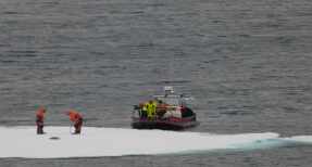
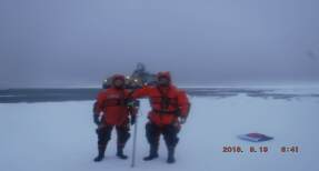
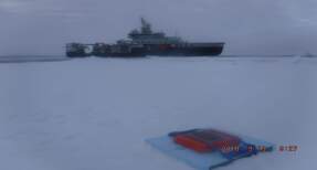
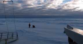
Figure 9: Deployment of the instruments 1 to 4 (left to right) in the Marginal Ice Zone, Northeast Barents sea. The concentration of ice increases from instrument 1 to 4, as visible in the pictures (1/10th, 3/10th, 9/10th, 10/10th). The instruments, equipped with buoys, are visible on the ice. Photos: credit Malte Müller and Lars R. Hole, Norwegian Meteorological Institute.

The temporal evolution of the battery level of the second instrument, which was the one which transmitted for the longest time, is presented in Fig. 10. As previously stated, the battery technology used inside the instruments is LiFePO4, and according to the datasheet the voltage of a fully charged battery is around 3.3V, and a fully discharged battery has a voltage of around 2.7V. As visible in Fig. 10, the battery barely depleted over the period of 12 days for which it was deployed. This is due to both the high power efficiency of the instrument, and the presence of the solar panel that provides energy at least for the first days of deployment, until the start of the polar night. It should be noted that temperature can also influence the battery voltage, which explains for apparent increases in battery level during some night periods. It is also apparent from Fig. 10 that the battery level was not the cause for the end of transmission. This confirms the quality of the power management solution and overall design, and is further discussed later in this section.

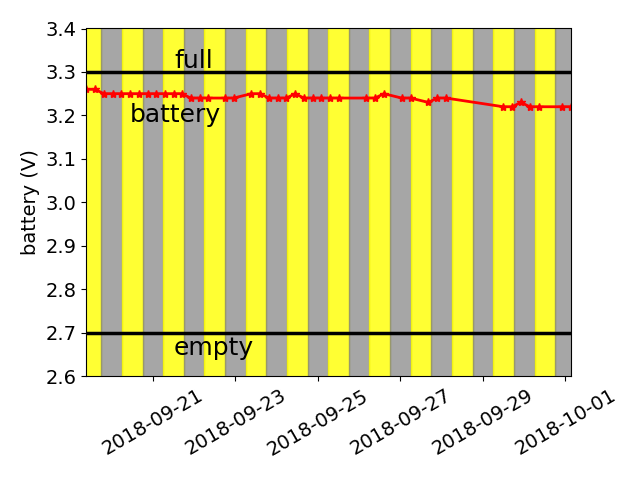
Figure 10: Time evolution of the battery level of instrument 2. The background color indicates time of the day: yellow is for 06:00 to 18:00, gray is for 18:00 to 06:00. The full and empty battery levels correspond to $3.3$V and $2.7$V, respectively. The battery level remains very high thanks to efficient power management and the presence of a solar panel.

The GPS information transmitted by all 4 instruments is presented in Fig. 11. As visible in Fig. 11, the trajectories of the instruments are well resolved until transmissions are lost. While some dropouts are present, a pattern of drift first to the West, then South and South East is clearly visible. During this period of 12 days, the instrument 2 (which survived the longest) drifted approximately $340$ km. This corresponds to the effect of the transpolar current, together with the forcing created by a storm present in the region September 24th and 25th. The data will be used for validating satellite tracking of ice drift and models, and these results also indicate that the instruments are valuable to use as drifters.

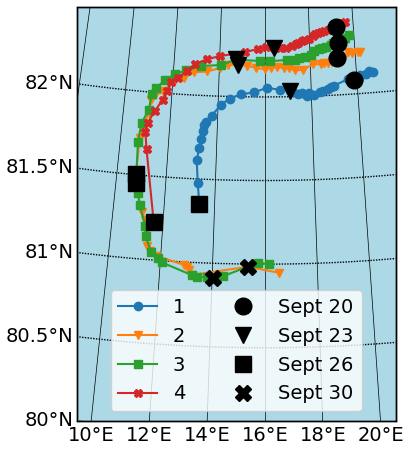
Figure 11: The drift of the instruments, as obtained from the GPS strings transmitted through Iridium. The symbols indicate the position of each instrument for the first transmission received on the corresponding day. A general drift pattern is clearly visible.

The core mission of the instruments is to provide in situ measurements of waves in ice. The spectrograms presenting the wave information transmitted by the instruments are visible in Fig. 12. Each spectrum is obtained using the Welch method, which is binned and compressed before being sent through Iridium, as described in the previous section. As visible in Fig. 12, the patterns for the waves in ice activity are coherent among sensors. In particular, there is an episode of high wave intensity between September 24th and September 25th, which corresponds to a storm in the region. Clear damping is visible as the waves propagate deeper into the ice, and the damping is higher for high frequency waves in agreement to what is expected from theoretical considerations. These data further cross-validate the approach and algorithms used for the measurements of waves in ice.

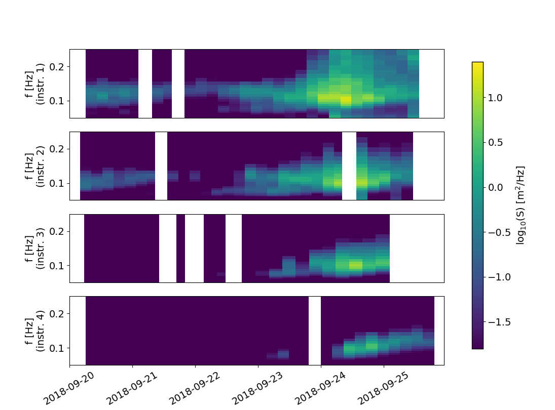
Figure 12: Spectrograms from all instruments, ordered going from the outer marginal zone (top) to the closed pack ice (bottom). Wave activity is clearly visible, and corresponds well with the duration of a storm in particular 24-09 to 25-09. Damping is clearly visible as the waves propagate deeper into the ice. This further validates the good functioning of the binning and transmission algorithm, and these data will be used for further calibration of waves in ice models.

Another cross-checking of the good quality of the on-board processing and data compression can be performed by comparing the scalar results transmitted, such as $H_{St}$, $H_{S0}$, $T_{z}$ and $T_{Z0}$, with similar values calculated from the reduced spectra sent through Iridium. This is illustrated for both quantities measuring wave height and period in Fig. 13. In this figure, the quantities obtained from the scalar values transmitted through Iridium are presented alongside those calculated from the reduced spectra (indicated by the ’proc’ suffix), following the methodology presented in the previous section. As visible on Fig. 13, we observe good agreement between quantities transmitted and calculated from the reduced spectra, which is an additional validation of both the methodology used and an indication that the resolution of the reduced spectra is enough to capture the dynamics of interest since the transmitted scalar quantities were computed over the whole, non under-sampled spectra. This figure also further validates the ability of the instrument to clearly detect changes in wave characteristics arising as a consequence of their propagation through the MIZ. Namely, both the wave damping and the preferential propagation of low frequency waves are clearly visible from comparing the results obtained by the different sensors. These data will be used to perform model calibration in later works.

Finally, the results obtained from the instrument further out of the MIZ can be compared with wave model predictions in the region. For this, we use the WAM wave model, run operationally by the Norwegian Meteorological Institute. As developing models for wave propagation in the MIZ is challenging and still a field of research, the model was set up so that ice with a concentration over 3/10th is considered as continent and completely stops wave propagation. Therefore, wave predictions are made only for instrument 1 and ignore the effect of the sparse ice floes present in the region. Similarly, the dynamic response of the ice floe is considered negligible to first order, i.e. we assume that the floe and attached IMU mostly follow the displacement of the water. The WAM wave model is a state-of-the art third generation spectral wave model (Hasselmann and others,, 1988). The basic physics and numerics of the WAM Cycle 4 wave model are described by Komen and others, (1994). The model solves the action balance equation, as do all third-generation spectral wave models (Tolman,, 1991; Booij and others,, 1999; Ardhuin and others,, 2010). In its current version, WAM 4.6.3 (freely available at http://mywave.github.io/WAM/), the source function integration scheme of Hersbach and Janssen, (1999) and the reformulated wave model dissipation source function (Bidlot and others,, 2007) are used. The spatial resolution is about 4 km, and the model covers the Norwegian Sea and the Barents Sea on a rotated spherical grid with boundary conditions from the European Centre for Medium-Range Weather Forecasts (see Breivik and others, (2009) for details on the boundary scheme). The two-dimensional spectrum is represented by 36 directions and 36 frequency bins, logarithmically spaced on 10% increments from 0.0345 Hz. The model is run daily to +66 hours. Here we have concatenated forecasts from consecutive runs to provide a continuous time series for comparison against our observations. The ice cover is taken from the operational weather prediction model and is updated daily. There will be discrepancies between the real ice cover and the modeled ice cover, and the model has no way of distinguishing between fractional ice cover and fast ice. For this reason, a hard ice boundary is set where the ice concentration exceeds 30%. Results are presented alongside the data from the IMUs in Fig. 13. As is visible there, the agreement between the model and in situ measurements is generally satisfactory considering the many coarse approximations used. This is one more external validation of the good functioning of the instruments.

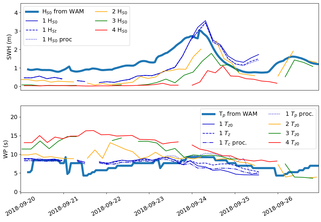
Figure 13: Comparison between the scalar quantities (significant wave height SWH and wave period WP according to different metrics, as described in section 2.2) transmitted by Iridium, the equivalent integral quantities calculated from the reduced spectra following the methodology presented in the previous section (quantities with suffix ’proc’), and results from the WAM waves model in the region close to the instrument outermost of the MIZ. The quality of the agreement between the different methods used for computing the wave height and period confirms both the methodology and under sampled spectra resolution chosen. In addition, the evolution of the wave properties as these travel through the MIZ are clearly visible. Namely, waves get attenuated (visible in the significant wave height), and the attenuation is larger for higher frequency waves (visible from the shift in the peak frequency of the waves). The quantities obtained from the reduced spectra are only presented for the first sensor to not overload the figure, but similar agreement is found for all instruments. Finally, reasonable agreement is obtained between the data reported by the instrument outermost in the MIZ and the predictions of the WAM model for the surrounding free-water wave field.

Regarding end of transmission, the battery level is clearly not to blame. Most likely, environmental conditions were at the origin of both transmission dropouts and finally loss of contact. The most probable causes are snow covering the antenna and shielding radio transmissions, polar bears damaging the instruments (3 polar bears were encountered during the deployment of the last two sensors), and ice breakup. This last factor is especially likely for the sensor furthest out from the MIZ, which lost contact when the storm was at its strongest. While little can be done about polar bears and ice breakup, we will consider mounting the antennas on a pole on the side of the main instrument in future iterations, in the hope that this may help getting contact with the satellite. However, this constitutes a tradeoff. Indeed, we believe that the reason why the instruments could survive for such a long duration despite polar bear activity lies in the low profile of the instruments, and probably a design featuring a case of larger vertical dimension or a pole may be more attractive and get damaged withing short time.

4 Conclusion and future work

Instruments performing in situ measurements of waves in ice were successfully designed in-house at the University of Oslo, tested and cross-tested during short field campaigns, and deployed in the MIZ in the Arctic, north of Svalbard during the Nansen legacy cruise in collaboration with the Norwegian Meteorological Institute. High quality data on ice drift and wave propagation in sea ice were obtained, which provides confidence in the engineering solutions employed in designing the instrument. These data will be used for further development and calibration of waves in ice models.

As both the hardware and software of the instrument are made available as an open source design (see Appendix A), this opens new possibilities for in situ measurements in the Arctic. Indeed, flexible and more affordable instruments may allow far more and higher quality measurements in harsh environments like the Arctic. Using open source code and PCBs allows for the reduction in the cost of the electronics to the point where the sensor performing the measurement represents over 50% of the total cost. In addition, flexibility means that scientists will be able to quickly design the instruments they need by adapting the baseline design to their own needs, rather than going through long and costly contracting with private companies. This means that the production of a small series of instruments adapted to the needs of a specific measurements campaign can take place within a few weeks, therefore, greatly reducing risks and costs.

We will continue to work on this design to provide simplified assembly processes for the end user and to further reduce costs and enhance functionality in the years to come, adopting the same kind of incremental refinements approach that was used for evolving from the first waves in ice loggers presented in 2016 to the present instruments. In particular, we will work further on isolating the IMU from magnetic disturbances induced by the battery and electronics, so that also directional information can be obtained in the future. We hope that sharing our design may participate in creating an ecosystem for open source instruments and benefit the community at large. Developing cost-effective instruments for in situ measurements in the Arctic is a promising avenue for collecting the data that several communities need, and may help towards better studies of these challenging, remote environments.

Appendix A: open source code and designs

All the designs and files used for the building of the instruments, including the PCB files ready for production, the code used on all processors (low power unit, logger, Raspberry Pi), and general instructions for assembling the instruments, are made available on the Github of the author under a MIT license that allows full re-use and further development (link:https://github.com/jerabaul29/LoggerWavesInIce_InSituWithIridium). All software and designs are based entirely on open source tools, so that the designs can be easily modified and built upon.

References

- Ardhuin and others, (2010) Ardhuin F, Rogers E, Babanin AV, Filipot JF, Magne R, Roland A, van der Westhuysen A, Queffeulou P, Lefevre JM, Aouf L and Collard F (2010) Semiempirical Dissipation Source Functions for Ocean Waves. Part I: Definition, Calibration, and Validation. J Phys Oceanogr, 40(9), 1917–1941 (doi: 10.1175/2010JPO4324.1)
- Ardhuin and others, (2017) Ardhuin F, Stopa J, Chapron B, Collard F, Smith M, Thomson J, Doble M, Blomquist B, Persson O, Collins III CO and others (2017) Measuring ocean waves in sea ice using sar imagery: A quasi-deterministic approach evaluated with sentinel-1 and in situ data. Remote sensing of Environment, 189, 211–222
- Bidlot and others, (2007) Bidlot J, Janssen P and Abdalla S (2007) A revised formulation of ocean wave dissipation and its model impact. ECMWF Technical Memorandum 509, European Centre for Medium-Range Weather Forecasts
- Booij and others, (1999) Booij N, Ris RC and Holthuijsen LH (1999) A third-generation wave model for coastal regions 1. Model description and validation. J Geophys Res, 104(C4), 7649–7666 (doi: 10.1029/98JC02622)
- Breivik and others, (2009) Breivik Ø, Gusdal Y, Furevik BR, Aarnes OJ and Reistad M (2009) Nearshore wave forecasting and hindcasting by dynamical and statistical downscaling. J Marine Syst, 78(2), S235–S243 (doi: 10/cbgwqd)
- Christensen and Broström, (2008) Christensen K and Broström G (2008) Waves in sea ice. Technical report, Norwegian Meteorological Institute
- Collins and others, (2015) Collins CO, Rogers WE, Marchenko A and Babanin AV (2015) In situ measurements of an energetic wave event in the arctic marginal ice zone. Geophysical Research Letters, 42(6), 1863–1870, ISSN 1944-8007 (doi: 10.1002/2015GL063063), 2015GL063063
- Doble and others, (2006) Doble M, Mercer D, Meldrum D and Peppe O (2006) Wave measurements on sea ice: developments in instrumentation. Annals of Glaciology, 44, 108–112 (doi: 10.3189/172756406781811303)
- Doble and Bidlot, (2013) Doble MJ and Bidlot JR (2013) Wave buoy measurements at the antarctic sea ice edge compared with an enhanced ECMWF wam: Progress towards global waves-in-ice modelling. Ocean Modelling, 70, 166 – 173, ISSN 1463-5003 (doi: http://dx.doi.org/10.1016/j.ocemod.2013.05.012), ocean Surface Waves
- Doble and others, (2017) Doble MJ, Wilkinson JP, Valcic L, Robst J, Tait A, Preston M, Bidlot JR, Hwang B, Maksym T and Wadhams P (2017) Robust wavebuoys for the marginal ice zone: Experiences from a large persistent array in the beaufort sea. Elem Sci Anth, 5
- Earle, (1996) Earle MD (1996) Nondirectional and directional wave data analysis procedures. DBC Tech. Doc 96-01, Natl. Data Buoy Cent., Natl. Oceanic and Atmos. Admin., U.S. Dep. of Commer., Washington, D. C.
- Hasselmann and others, (1988) Hasselmann S, Hasselmann K, Bauer E, Janssen PAEM, Komen GJ, Bertotti L, Lionello P, Guillaume A, Cardone VC, Greenwood JA, Reistad M, Zambresky L and Ewing JA (1988) The WAM model—a third generation ocean wave prediction model. J Phys Oceanogr, 18, 1775–1810 (doi: 10/bhs3rr)
- Hersbach and Janssen, (1999) Hersbach H and Janssen P (1999) Improvement of the short-fetch behavior in the Wave Ocean Model (WAM). J Atmos Ocean Tech, 16(7), 884–892 (doi: {10.1175/1520-0426(1999)016<0884:IOTSFB>2.0.CO;2})
- Horvat and Tziperman, (2015) Horvat C and Tziperman E (2015) A prognostic model of the sea-ice floe size and thickness distribution. The Cryosphere, 9(6), 2119–2134
- Horvat and others, (2016) Horvat C, Tziperman E and Campin JM (2016) Interaction of sea ice floe size, ocean eddies, and sea ice melting. Geophysical Research Letters, 43(15), 8083–8090
- Hwang and others, (2017) Hwang B, Wilkinson J, Maksym E, Graber HC, Schweiger A, Horvat C, Perovich DK, Arntsen AE, Stanton TP, Ren J and others (2017) Winter-to-summer transition of arctic sea ice breakup and floe size distribution in the beaufort sea. Elementa Science of the Anthropocene, 5
- Kohout and others, (2014) Kohout A, Williams M, Dean S and Meylan M (2014) Storm-induced sea-ice breakup and the implications for ice extent. Nature, 509(7502), 604
- Kohout and others, (2015) Kohout AL, Penrose B, Penrose S and Williams MJM (2015) A device for measuring wave-induced motion of ice flows in the antarctic marginal ice zone. Annals of Glaciology, 56(69), 415–424 (doi: 10.3189/2015AoG69A600)
- Komen and others, (1994) Komen GJ, Cavaleri L, Donelan M, Hasselmann K, Hasselmann S and Janssen PAEM (1994) Dynamics and Modelling of Ocean Waves. Cambridge University Press, Cambridge
- Kuik and others, (1988) Kuik A, Van Vledder GP and Holthuijsen L (1988) A method for the routine analysis of pitch-and-roll buoy wave data. Journal of physical oceanography, 18(7), 1020–1034
- Liu and Mollo-Christensen, (1988) Liu AK and Mollo-Christensen E (1988) Wave propagation in a solid ice pack. Journal of Physical Oceanography, 18(11), 1702 – 1712, ISSN 0022-3670 (doi: 10.1175/1520-0485)
- Liu and others, (1991) Liu AK, Holt B and Vachon PW (1991) Wave propagation in the marginal ice zone: Model predictions and comparisons with buoy and synthetic aperture radar data. Journal of Geophysical Research: Oceans, 96(C3), 4605–4621
- Longuet-Higgins, (1963) Longuet-Higgins MS (1963) Observations of the directional spectrum of sea waves using the motions of a floating buoy. Ocean wave spectra
- Marchenko and others, (2013) Marchenko A, Morozov E and Muzylev S (2013) Measurements of sea-ice flexural stiffness by pressure characteristics of flexural-gravity waves. Annals of Glaciology, 54(64), 51–60 (doi: doi:10.3189/2013AoG64A075)
- Marchenko and others, (2017) Marchenko A, Rabault J, Sutherland G, Collins COI, Wadhams P and Chumakov M (2017) Field observations and preliminary investigations of a wave event in solid drift ice in the barents sea. In 24th International Conference on Port and Ocean Engineering under Arctic Conditions
- Marchenko and others, (2019) Marchenko A, Wadhams P, Collins C, Rabault J and Chumakov M (2019) Wave-ice interaction in the north-west barents sea. Applied Ocean Research, 90, 101861, ISSN 0141-1187 (doi: https://doi.org/10.1016/j.apor.2019.101861)
- Pfirman and others, (1995) Pfirman S, Eicken H, Bauch D and Weeks W (1995) The potential transport of pollutants by arctic sea ice. Science of The Total Environment, 159(2–3), 129 – 146, ISSN 0048-9697 (doi: http://dx.doi.org/10.1016/0048-9697(95)04174-Y)
- Rabault, (2018) Rabault J (2018) An investigation into the interaction between waves and ice. PhD Thesis, University of Oslo
- Rabault and others, (2016) Rabault J, Sutherland G, Ward B, Christensen KH, Halsne T and Jensen A (2016) Measurements of waves in landfast ice using inertial motion units. IEEE Transactions on Geoscience and Remote Sensing, 54(11), 6399–6408, ISSN 0196-2892 (doi: 10.1109/TGRS.2016.2584182)
- Rabault and others, (2017) Rabault J, Sutherland G, Gundersen O and Jensen A (2017) Measurements of wave damping by a grease ice slick in svalbard using off-the-shelf sensors and open-source electronics. Journal of Glaciology, 1–10 (doi: 10.1017/jog.2017.1)
- Rabault and others, (2019) Rabault J, Sutherland G, Jensen A, Christensen KH and Marchenko A (2019) Experiments on wave propagation in grease ice: combined wave gauges and particle image velocimetry measurements. Journal of Fluid Mechanics, 864, 876–898 (doi: 10.1017/jfm.2019.16)
- Reigstad and others, (2017) Reigstad M, Eldevik T and Gerland S (2017) The nansen legacy. scientific exploration and sustainable management beyond the ice edge. overall project plan. https://arvenetternansen.com/wp-content/uploads/2018/02/Nansen-Legacy-3.0-WEB-2.pdf, accessed 22/11/18
- Rigor and Colony, (1997) Rigor I and Colony R (1997) Sea-ice production and transport of pollutants in the laptev sea, 1979–1993. Science of The Total Environment, 202(1–3), 89 – 110, ISSN 0048-9697 (doi: http://dx.doi.org/10.1016/S0048-9697(97)00107-1), environmental Radioactivity in the Arctic
- Roach and others, (2018) Roach LA, Horvat C, Dean SM and Bitz CM (2018) An emergent sea ice floe size distribution in a global coupled ocean–sea ice model. Journal of Geophysical Research: Oceans
- Specialist Committee on Stability in Waves of the 28th ITTC, (2017) Specialist Committee on Stability in Waves of the 28th ITTC (2017) Confidence intervals for significant wave height and modal period. Technical report, International Towing Tank Conference, available at https://www.ittc.info/media/8099/75-02-07-014.pdf
- Squire and others, (1995) Squire V, Dugan JP, Wadhams P, Rottier PJ and K A (1995) Of ocean waves and sea-ice. Annual Review of Fluid Mechanics, 27, 115 – 168 (doi: http://10.1146/annurev.fl.27.010195.000555)
- Squire, (2018) Squire VA (2018) A fresh look at how ocean waves and sea ice interact. Phil. Trans. R. Soc. A, 376(2129), 20170342
- Stopa and others, (2018) Stopa J, Ardhuin F, Thomson J, Smith MM, Kohout A, Doble M and Wadhams P (2018) Wave attenuation through an arctic marginal ice zone on 12 october 2015: 1. measurement of wave spectra and ice features from sentinel 1a. Journal of Geophysical Research: Oceans, 123(5), 3619–3634
- Sutherland and Rabault, (2016) Sutherland G and Rabault J (2016) Observations of wave dispersion and attenuation in landfast ice. Journal of Geophysical Research: Oceans, 121(3), 1984–1997, ISSN 2169-9291 (doi: 10.1002/2015JC011446)
- Sutherland and others, (2017) Sutherland G, Rabault J and Jensen A (2017) A method to estimate reflection and directional spread using rotary spectra from accelerometers on large ice floes. Journal of Atmospheric and Oceanic Technology, 34(5), 1125–1137 (doi: 10.1175/JTECH-D-16-0219.1)
- Sutherland and others, (2019) Sutherland G, Rabault J, Christensen KH and Jensen A (2019) A two layer model for wave dissipation in sea ice. Applied Ocean Research, 88, 111 – 118, ISSN 0141-1187 (doi: https://doi.org/10.1016/j.apor.2019.03.023)
- Sutherland and Dumont, (2018) Sutherland P and Dumont D (2018) Marginal ice zone thickness and extent due to wave radiation stress. Journal of Physical Oceanography, 48(8), 1885–1901 (doi: 10.1175/JPO-D-17-0167.1)
- Tolman, (1991) Tolman HL (1991) A Third-Generation Model for Wind Waves on Slowly Varying, Unsteady, and Inhomogeneous Depths and Currents. J Phys Oceanogr, 21(6), 782–797 (doi: 10/ddxwxn)
- Tucker and Pitt, (2001) Tucker M and Pitt E (2001) Waves in Ocean Engineering. Elsevier ocean engineering book series, Elsevier, ISBN 9780080435664
- Vectornav Corporation, (2018) Vectornav Corporation (2018) VN100 product specification. https://www.vectornav.com/docs/default-source/documentation/vn-100-documentation/PB-12-0002.pdf?sfvrsn=9f9fe6b9_18, accessed 20/12/18
- Wadhams, (1979) Wadhams P (1979) Field experiments on wave-ice interaction in the labrador and east greenland currents, 1978. Polar Record, 19, 373–376, ISSN 1475-3057 (doi: 10.1017/S0032247400002138)
- Wadhams and Doble, (2009) Wadhams P and Doble MJ (2009) Sea ice thickness measurement using episodic infragravity waves from distant storms. Cold Regions Science and Technology, 56(2–3), 98 – 101, ISSN 0165-232X (doi: http://dx.doi.org/10.1016/j.coldregions.2008.12.002)
- Wadhams and Squire, (1980) Wadhams P and Squire VA (1980) Field experiments on wave-ice interaction in the bering sea and greenland waters, 1979. Polar Record, 20, 147–153, ISSN 1475-3057 (doi: 10.1017/S0032247400003144)
- Wang and Shen, (2010a) Wang R and Shen HH (2010a) Experimental study on surface wave propagating through a grease–pancake ice mixture. Cold Regions Science and Technology, 61(2–3), 90 – 96, ISSN 0165-232X (doi: http://dx.doi.org/10.1016/j.coldregions.2010.01.011)
- Wang and Shen, (2010b) Wang R and Shen HH (2010b) Gravity waves propagating into an ice-covered ocean: A viscoelastic model. Journal of Geophysical Research: Oceans, 115(C6), n/a–n/a, ISSN 2156-2202 (doi: 10.1029/2009JC005591)
- Weber, (1987) Weber JE (1987) Wave attenuation and wave drift in the marginal ice zone. Journal of Physical Oceanography, 17(12), 2351–2361 (doi: 10.1175/1520-0485(1987)017<2351:WAAWDI>2.0.CO;2)
- Young, (1995) Young I (1995) The determination of confidence limits associated with estimates of the spectral peak frequency. Ocean Engineering, 22(7), 669 – 686, ISSN 0029-8018 (doi: https://doi.org/10.1016/0029-8018(95)00002-3)
- Young, (1986) Young IR (1986) Probability distribution of spectral integrals. Journal of Waterway, Port, Coastal, and Ocean Engineering, 112(2), 338–341 (doi: 10.1061/(ASCE)0733-950X(1986)112:2(338))
- Zhao and Shen, (2015) Zhao X and Shen HH (2015) Wave propagation in frazil/pancake, pancake, and fragmented ice covers. Cold Regions Science and Technology, 113, 71 – 80, ISSN 0165-232X (doi: http://dx.doi.org/10.1016/j.coldregions.2015.02.007)