The secondary transit of the hot Jupiter WASP-121b at 2 $\mu$m

Ground-based observations of the secondary transit in the 2MASS K band are presented for the hot Jupiter WASP-121b. These are the first occultation observations of an extrasolar planet carried out with an instrument attached to a $1$ m-class telescope (SMARTS’ $1.3$ m). We find a highly significant transit depth of $(0.228\pm 0.023)$%. Together with the Hubble Space Telescope near infrared emission spectrum, current data support more involved atmosphere models with species producing emission/absorption features, rather than simple smooth black body emission. Analysis of the time difference between the primary and secondary transits and the durations of these events yield an eccentricity of $e=0.0207\pm 0.0153$, which is consistent with the earlier estimates of low/zero eccentricity, but with a smaller error. Together with the existing K-band data on other systems, WASP-121b lends further support to the lack of efficient heat transport between the day and night sides for nearly all Hot Jupiters.

1 Introduction

When combined with other pieces of information (such as planet mass), the low thermal radiation of extrasolar planets is a direct evidence of their substellar nature. In addition to this independent verification, measuring the radiation spectrum yields a wealth of information on atmospheric structure and basic orbital parameters. Due to their low temperatures (relative to their host stars), the best chance of detection is obviously in the infrared. From the first detection, employing the mid-infrared instrument of the Spitzer Space Telescope by Deming et al. (deming2005 (2005)), many systems have been observed not only by space-based, but also by ground-based instruments attached to 4-meter class telescopes. Here we report the multiple detection of the secondary transit of the Hot Jupiter (HJ) WASP-121b in the 2MASS K band by A Novel Dual Imaging CAMera (ANDICAM) attached to the $1.3$ m telescope of the SMARTS Consortium.

The transiting extrasolar planetary system WASP-121 was discovered by Delrez et al. (delrez2016 (2016)) using the wide-field telescopes of the SuperWASP project (Pollacco et al. pollacco2006 (2006), see also Anderson et al. anderson2018 (2018) for the latest update). The analysis of these and the subsequent spectroscopic followup observations revealed that WASP-121b is a very hot Jupiter, with a maximum photospheric temperature above $3000$ K. This is not surprising, since the planet orbits an F star rather close, with a period of $1.27$ days. The close orbit, the extended planet’s radius of $R_{\rm p}=1.87\leavevmode\nobreak\ R_{\rm J}$ with standard mass of $M_{\rm p}=1.18\leavevmode\nobreak\ M_{\rm J}$ imply rather strong tidal dissipation, leading to Roche-lobe filling and then to a speedy disruption within some hundred million years, assuming a stellar tidal dissipation factor $Q_{\rm star}<10^{8}$ (see Delrez et al. delrez2016 (2016)). In addition, the planet has probably experienced a strong dynamical interaction with some nearby third body, as can be inferred from the large projected spin-orbit angle of $258^{\circ}\pm 5^{\circ}$ (see Delrez et al. delrez2016 (2016)). Interestingly, secondary transits were observed multiple times by the same authors in the Sloan-z’ band by the $60$ cm TRAPPIST telescope – to our knowledge, this is the first occultation detection from the ground by a telescope of this size. The significant detection of the occultation depth of a mere $(0.060\pm 0.013)$% resulted in the first direct estimation of the planet temperature. Important followup observations (both during the primary and secondary transits) have been made by Evans et al. (evans2016 (2016, 2017, 2018)) by using the Hubble Space Telescope’s Wide Field Camera 3 in the near infrared, Spitzer’s IRAC detector at $3.6$ $\mu$m and HST/STIS in the UV. These data indicate a weak $H_{2}O$ emission during occultation and absorption during transit, implying temperature inversion due to some high-altitude absorber. In spite of the successful fit of the HST emission spectrum, and quite currently the transmission spectrum observed by the same instrument, the authors caution for the non-uniqueness of the solution (e.g., type of absorber, precision of the fit at different wavelengths, etc.). These issues are not unique to WASP-121b, they are also present in other very hot Jupiters (e.g., WASP-33b, Kepler-13Ab – see Parmentier et al. parmentier2018 (2018)). In spite of the considerable progress made in the past ten years, there is a substantial lack of understanding the relations between the physical parameters of the systems and the thermal properties of their planets (see the uniform analysis by Adams & Laughlin adams2018 (2018) of 10 systems with full infrared phase curves).

The purpose of this work is to add a flux value to the emission spectrum of WASP-121b at a single waveband and thereby increase the number of constraints on future atmosphere modeling of the planet. Furthermore, timing estimates are presented to give more stringent limits on the orbital eccentricity, a valuable parameter for the analysis of the dynamical history of the system.

2 Observations and the method of analysis

Photometric observations in the 2MASS K and Cousins I bands (effective wavelengths of $2.2$ $\mu$m and $0.8$ $\mu$m, respectively) have been made by using the ANDICAM instrument in a beam-splitting mode, allowing simultaneous data acquisition in the two bands. On each night, the target was monitored continuously, by allowing ample amount of pre- and after-event time (permitted by the actual sky position) to reliably fix the out-of-transit (OOT) baseline for the event lasting almost for $3$ hours. An exposure time of $15$–$20$ s was used, resulting in an overall cadence of $70$–$500$ s, due to the overheads, related to read-outs, varying movements due to dithering and other data acquisition steps. The observing log with some associated parameters is given in Table 1.

Table 1: List of secondary transit observations of WASP-121b in the near infrared.

Date [UT]	$T_{\rm occ}$ [HJD]	$T_{\rm tot}$ [hours]	$N_{\rm tot}$
02/26/2016	2457444.64855	4.86	177
01/11/2017	2457764.65485	6.13	203
01/25/2017	2457778.67903	6.64	205

Notes:
$T_{\rm occ}$ stands for the time of the center of occultation as estimated from the ephemeris given by Delrez et al. (delrez2016 (2016)) for the primary transit in their Table 4. $T_{\rm tot}$ and $N_{\rm tot}$ are the total observing time and data points gathered.

For the K-band observations dithering was used to decrease the higher sensitivity against detector non-uniformity in the near infrared. We found this method useful, as we did not have a priori information on pixel sensitivity. Admittedly, this method has also some risk, since by testing different parts of the CCD, we may bump into bad positions, leading to light curves of larger scatter associated with the particular dither position. All in all, we think that our strategy has proven to be useful and led to a higher quality result at the end.

By stacking several images, we show the dither pattern in Fig. 1 for one of the nights. The number of dither positions changed from night to night, and their durations were also not the same. The image (that has already been corrected for flat field) spectacularly exhibits sequences of rings, reminiscent of the trace of some earlier drops of dew. In spite of their high visibility, their effect has been proven to be less damaging for the data quality than the varying pixel sensitivity (that is considerable more difficult to spot, because they lack the type of spatial correlation the rings have).

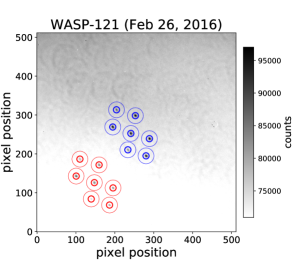
Figure 1: Dithering pattern used during the near infrared observations. The image shows the $2.4^{\prime}\times 2.4^{\prime}$ FOV of the ANDICAM near infrared camera, attached to the $1.3$ m telescope of the SMARTS Consortium. The target (WASP-121=2MASS 07102406-3905506) is in the middle, the comparison star 2MASS 07102364-3905561 is in the lower left corner. North is on the top West is on the left. Circles around the target and the comparison star show the aperture sizes used to estimate the star and background fluxes.

In producing the photometric time series to be used in the derivation of the basic occultation parameters, we proceed as follows. First we compute simple relative fluxes at various, but fixed circular apertures from $10$ to $20$ pixel radii with an increment of $2$ pixels. After a lot of experimenting, and inspecting the final product of the full detrending procedure to be described below, we find that the aperture with the pixel radius of $16$ yields a light curve with the smallest scatter. All results presented in this paper refer to the above aperture size.

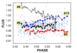
Figure 2: Simple photometric flux ratios ordered by the orbital period (pale dots). Some dithers are annotated to see the nightly trends (or the lack of them, i.e., #9). Dither #6 (gray dots) is plotted also after employing zero point shift and detrending by the position vector (black dots, see Sect. 2 for details).

By using the relative fluxes (target over comparison star flux, hereafter raw flux) and folding the data with the orbital period, we can examine if we can see some sign of an occultation event. The result is shown in Fig. 2. The pale dots show that the raw fluxes are very noisy, and the event with the expected depth of $0.1$–$0.2$% is hopelessly buried in the noise. We can find out the reason of this somewhat unexpected high level of noise by examining the individual light curves (LCs) associated with the various dither positions. Indeed, we see from the highlighted LCs that there is a strong dependence on the dither position, leading to both zero point shifts and nightly trends. Therefore, (not entirely unexpectedly), we must employ some detrending method that is likely the cause of the trends and zero point shifts. The detrending step is vital and therefore quite common in the extraction of planetary signals in general, and, in particular, in the derivation of wavelength-dependent transit depths for the exquisite accuracy needed to estimate emission or transmission spectra (e.g., Stevenson et al. stevenson2012 (2012); Kreidberg et al. kreidberg2015 (2015)).

It is well-known that ground-based instruments detect stellar light deformed by the multiplicative noise and systematics originating from the Earth’s atmosphere and from the environment/instrument. In addition, we also have an additive noise source, coming from the sky background

$$F = F_{0}\times T_{\rm atm}\times T_{\rm env}+F_{\rm bg}\hskip 2.84526pt,$$ (1)

where $F$ is the detected, $F_{0}$ is the true stellar flux. The transmission functions of the Earth’s atmosphere and the instrument are denoted by $T_{\rm atm}$ and $T_{\rm env}$, respectively, whereas the background flux by $F_{\rm bg}$. In traditional photometric reductions the atmospheric and instrumental effects are filtered out with the aid of comparison stars near the target, by using the assumption of the close similarity in the transmission functions for the target and its neighboring companions. However, when higher accuracy is required, this method usually fails, because of the lack of complete equivalence between the transmission functions of the target and the comparison stars (and, for faint targets, there is also the issue of the presence of the additive background noise).

Due to the lack of obvious exact solution of the problem (similarly to the methodology followed in other studies, e.g., Bakos et al. bakos2010 (2010), Delrez et al. delrez2016 (2016)), we opt to an approximate one. Here we take the logarithm of the target to comparison star flux ratios $F/F^{\rm c}$, and fit the data with the linear combination of the presumed signal and certain external photometric parameters (e.g., position, PSF width). In addition, we treat each LC of the different dither positions individually, with particular zero points and trends (but with the same underlying signal). That is, we Least Square minimize the following expression

$$\mathcal{D} = \sum_{j=1}^{M}\sum_{i=1}^{N_{\rm j}}w_{\rm j}\bigg{[}\log\Bigg{(}{F_{\rm j}(i)\over F_{\rm j}^{\rm c}(i)}\Bigg{)}-E_{\rm j}(i)\bigg{]}^{2}\hskip 5.69054pt,$$ (2)

$$E_{\rm j}(i) = a_{0,\rm j}+a_{x,\rm j}X_{\rm j}(i)+a_{y,\rm j}Y_{\rm j}(i)+A\log(F_{\rm trap}(i))\hskip 2.84526pt.$$ (3)

Here all data are sorted by the orbital phase. We assume that there are $M$ dither positions altogether with $N_{\rm j}$ data points at the $j$-th dither. Since our extensive tests showed that neither arbitrary polynomial nor additional external parameters are needed to reach a high signal-to-noise ratio ($S/N$) detection, we use only the pixel position components $(X,Y)$ of the target to correct for instrumental effects. The stellar flux during the occultation is approximated by a trapezoidal function $F_{\rm trap}$ with fixed ingress/egress time, duration and transit center of $0.015$, $0.120$ and $2457764.65485$ days, respectively, corresponding to those given by Delrez et al. (delrez2016 (2016)). The weights $\{w\}$ are constant for the same dither index and proportional to the reciprocal of the variance of the residuals around the best-fitting trapezoidal. Since the solution is not known, the weights are iterated during the process of solution. At the end, the data are converted back to relative intensities, with an OOT normalization of $1.0$ for the fitted trapezoidal. The error of the occultation depth is computed as follows

$$\sigma(\delta_{\rm occ})=\Bigg{(}1-{N_{\rm p}\over N}\Bigg{)}^{-1/2}\Bigg{(}{s_{14}\over N_{14}^{2}}+{s_{\rm oot}\over N_{\rm oot}^{2}}\Bigg{)}^{1/2}\hskip 2.84526pt,$$ (4)

where $s_{14}$ and $s_{\rm oot}$ are sums of the squared residuals in the in- and out-of-transit phases, respectively. Akin to these are the number of data points $N_{14}$ and $N_{\rm oot}$. The factor in front (with $N_{\rm p}$ number of the parameters fitted to $N$ total number of data points) is for the debiasing of the error due to the decrease of the degrees of freedom, because of parameter fitting. The $S/N$ of the detection is the ratio of the average transit depth to the above error

$$S/N={1\over\sigma(\delta_{\rm occ})}{1\over N_{14}}\sum_{i=1}^{N_{14}}F_{\rm trap}(i)\hskip 2.84526pt.$$ (5)

3 Occultation parameters

First we fix all secondary transit parameters (but the occultation depth) by assuming circular orbit and the validity of the parameters derived for the primary transit by Delrez et al. (delrez2016 (2016)). Following the procedure described in Sect. 2, we compute the best fitting occultation depth under various conditions, concerning the number of points clipped and the dither LCs omitted. The result is shown in Table. 2. Except perhaps for the extreme choices of data trimming parameters ($N_{\rm dith}^{\rm cut}$ and $N_{\sigma}^{\rm cut}$), the occultation depth is relative stable. To avoid too sparsely populated dither LCs, and not to ‘overtrim’ the data, we opt for the case of $N_{\rm dith}^{\rm cut}=10$ and $N_{\sigma}^{\rm cut}=4$. The folded LC obtained in this way is shown in Fig. 3. The resulting secondary transit depth is $0.00228\pm 0.00023$.

Table 2: Occultation depths for WASP-121 in the 2MASS K band

$N_{\rm dith}^{\rm cut}$	$N_{\sigma}^{\rm cut}$	$N_{\rm par}$	$N$	$S/N$	$\sigma_{\rm fit}$	$\delta_{\rm occ}$
00	$\infty$	$70+\phantom{0}0$	$585$	$8.1$	$0.00272$	$0.00212$
00	$5$	$70+\phantom{0}8$	$585$	$8.4$	$0.00264$	$0.00215$
00	$4$	$70+11$	$585$	$8.8$	$0.00264$	$0.00224$
00	$3$	$70+25$	$585$	$9.2$	$0.00256$	$0.00227$
10	$\infty$	$61+\phantom{0}0$	$561$	$8.2$	$0.00275$	$0.00217$
10	$5$	$61+\phantom{0}8$	$561$	$8.5$	$0.00266$	$0.00220$
10	$4$	$61+11$	$561$	$8.9$	$0.00266$	$0.00228$
10	$3$	$61+25$	$561$	$9.3$	$0.00257$	$0.00231$
15	$\infty$	$52+\phantom{0}0$	$520$	$8.2$	$0.00281$	$0.00231$
15	$5$	$52+\phantom{0}8$	$520$	$8.6$	$0.00270$	$0.00233$
15	$4$	$52+11$	$520$	$8.9$	$0.00270$	$0.00243$
15	$3$	$52+25$	$520$	$9.3$	$0.00260$	$0.00244$

Notes:
$N_{\rm dith}^{\rm cut}$ is the lower limit on the number of data points per dither position. $N_{\sigma}^{\rm cut}$ is the number of standard deviations used in the clipping of the data points. $N_{\rm par}$ is the number of parameters fitted, plus the number of data points omitted ($N_{\rm p}$ in Eq. 4 includes both of these). Items in the last two columns (unbiased estimates of the standard deviation of the residuals and occultation depth) refer to the OOT$=1$ normalization as described in Sect. 2.

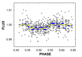
Figure 3: Systematics-filtered folded flux ratios normalized to $1.0$ in the out-of-transit part. Average fluxes (in $30$ phase bins) are shown by blue dashes, the best fitting trapezoidal secondary transit approximation is plotted by yellow continuous line.

To check the level of the systematics filtering, we compute the autocorrelation function (ACF) of the residuals after subtracting the best-fitting trapezoidal as shown in Fig. 3. In the units of the orbital period, the ACF is computed with steps of $0.00123$ up to $0.115$, i.e. close to the length of the full transit event. As a sanity check, we also compute the ACF for many Gaussian white noise realizations. The result is shown in Fig. 4. We see that the residuals are almost uncorrelated. The basic correlation length is under $\sim 0.005$ in the units of the orbital period. This value is less than one half of the ingress duration. It seems that the de-correlation method applied yields nearly white noise residuals, supporting the validity of the pure statistical error estimation given by Eq. 4. We also note that similar short-time-scale correlations are observable in other studies dealing with systematics, in particular in the analysis of the HST data by Evans et al. (evans2017 (2017)).

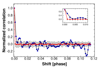
Figure 4: Blue dots: autocorrelation function (ACF) of the residuals of the trapezoidal fit to the final dataset shown in Fig. 3. Red dots: ACF of generated uncorrelated noise. Error bars are for the standard deviations of the the ACF values of the random datasets. The time lag is given in the units of the orbital period. The inset shows the immediate neighborhood of ACF at zero time shift (given in the units of the orbital period).

Although the noise is rather high, the relative large number of data points led to a high-$S/N$ detection. Therefore, it is tempting to see if our assumption on the applicability of the primary transit parameters is really held, and if there is a chance to further constrain the eccentricity by the best-fitting occultation center and event duration. To this aim we map the quality of the fit as a function of $\Delta T_{\rm c}$ (tested occultation center time minus the one calculated from the primary transit with the assumption of circular orbit) and $t14$ (occultation duration).

In addition to our data, to examine further the issue of eccentricity, the secondary transit data of Delrez et al. (delrez2016 (2016)) are also investigated. Since the observations were made in the Sloan z’ band, the signal is considerably shallower than in the 2MASS K ($K_{\rm s}$) band. Nevertheless, the number of data points ($6260$ flux measurements on seven nights) compensates for this, and yields a confident detection of $S/N=7.5$, with $\delta_{\rm occ}=0.000697\pm 0.000081$ and a residual standard deviation of $0.003190$. This depth is larger by $0.000096$ than the one derived by Delrez et al. (delrez2016 (2016)), but the difference is within $1\sigma$, and could be accounted for by the lower number of detrending parameters used in our code. We found it satisfactory to use only the pixel coordinates, and avoid to correct with a polynomial and other parameters, since these do not yield an appreciable improvement in the quality of the fit, and, in addition, may lead to a depression of the occultation depth.

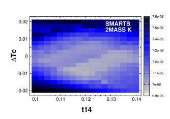
Figure 5: Intensity plot for the unbiased estimate of the variance of the residuals between the data and the occultation model scanned in the parameter space of the displacement of the occultation center $\Delta T_{\rm c}$ and the duration of the event $t14$. We employ iterative $4\sigma$ clipping to find the best solution for each parameter combination.

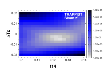
Figure 6: As in Fig. 5, but for the TRAPPIST data. The better contrast (in spite of the larger residual scatter) of the best solution is likely accounted for by the more than ten times larger number of data points than for the SMARTS observations.

The ($\Delta T_{\rm c}$, $t14$) maps are shown in Figs. 5 and 6 for the $K_{\rm s}$ and Sloan z’ data, respectively. As expected, the topology of both maps confirms the rather small (if any) deviations from the parameters predicted by the primary transit with the assumption of circular orbit. Furthermore, the Sloan z’ data are more restrictive than the $K_{\rm s}$ data, even though the $S/N$ value is higher for the latter. This is because the parameter maps yield information also on the sensitivity of the solution on the neighboring parameter values and not only on a specific combination of the parameters, that might be better or worse, depending on the functional form of the variance on these parameters and noise level. The better quality of the Sloan z’ data is also visible from the nearly three times smaller error of the derived occultation depth.

Table 3: Observed secondary transit times for WASP-121b

Dataset	$T_{\rm occ}$ [BJD]	$O-C$ [d]	$t14$	Source
SMARTS (K)	2457764.6469	$-0.0080$	$0.116$	KOV18
	$\pm 0.0023$	$\pm 0.0023$	$\pm 0.005$
TRAPPIST (z’)	2456762.5594	$-0.0040$	$0.128$	KOV18
	$\pm 0.0027$	$\pm 0.0027$	$\pm 0.007$
HST (’white’)	2457703.4588	$0.0004$	$-$	EVA17
	$\pm 0.0004$	$\pm 0.0004$
Spitzer (3.6)	2457783.7774	$-0.0013$	$-$	EVA17
	$\pm 0.0007$	$\pm 0.0007$

Notes:
EVA17: Evans et al. (2017) – KOV18: this paper (the source of the TRAPPIST data is Delrez et al. delrez2016 (2016)) – The O-C values are computed in respect of the ephemerides predicted from the primary transit as given by Delrez et al. (delrez2016 (2016)), assuming circular orbit. – See text for the equality of the errors on $T_{\rm occ}$ and $O-C$. – Evans et al. (evans2017 (2017)) do not supply occultation duration values.

The currently available secondary transit parameters are summarized in Table 3. In the case of the KOV18 items the errors have been computed in the following way. Once the best-fitting trapezoidal was found, we added Gaussian white noise with the observed standard deviations of the residuals corresponding to this solution, and then the best-fitting trapezoidal to these simulated data was searched for. By repeating the process $500$ times we arrived to statistically stable estimates of the formal errors. The ingress/egress time was always fixed to the observed values given by the primary transit data of Delrez et al. (delrez2016 (2016)), and we did the same also with the remaining parameters, depending which parameter was tested for errors (e.g., in the case of the occultation center, we fixed the duration and the ingress/egress times). Although this approach is primarily dictated by keeping the execution time within a reasonable limit, our error estimates for the moment of the occultation time is in perfect agreement with the one predicted by the analytic formula of Deeg & Tingley (deeg2017 (2017)). The errors of $O-C$ are taken equal to those of $T_{\rm occ}$, because the errors of the computed occultation times (C) have been proven to be negligible.

We see that the available observations suggest a small (or zero) eccentricity. Since the more precise estimation requires also the knowledge of the transit duration, the lack of this parameter for the most accurate HST and Spitzer observations makes us unable to include these data in the analysis. Therefore, we use only the occultation parameters derived from the SMARTS and TRAPPIST observations.

Following Winn (winn2010 (2010)), by omitting the negligible inclination effect, we use the following formula to estimate the eccentricity

$$e=\Bigg{[}\Bigg{(}{\pi\over 2}{\Delta T_{\rm c}\over P}\Bigg{)}^{2}+{\Bigg{(}{{r14-1}\over{r14+1}}\Bigg{)}^{2}}\Bigg{]}^{1\over 2}\hskip 2.84526pt,$$ (6)

where $P$ is the orbital period, $\Delta T_{\rm c}$ is the observed time of the occultation center minus the predicted time from the primary transit, assuming zero eccentricity; $r14=t14(\rm occ)/t14(\rm tra)$, that is the ratio of the secondary and primary transit durations. Assuming that the errors are independent on the transit times and durations both for the primary and the secondary transits and that these errors are also uncorrelated with the error of the period, we can use the above equation to estimate the eccentricity and its pure statistical error. For the primary transit and period we take the values given in Table 4 of Delrez et al. (delrez2016 (2016)). For the secondary transit we use the values shown in Table 3 of this paper. Errors are assumed to be Gaussian. Then, Eq. 6 yields $e=0.0207\pm 0.0153$ if we use the SMARTS and $e=0.0314\pm 0.0222$, if we use the TRAPPIST data. These eccentricity values are also tested by using the primary transit center values of Evans et al. (evans2018 (2018)) for the HST/STIS G430Lv2 band (we get very similar results also for the other bands). We note that this test is not entirely consistent, since we use the transit duration value of Delrez et al. (delrez2016 (2016)), because, Evans et al. (evans2018 (2018)) do not give this parameter for their data. We get for the SMARTS and TRAPPIST data, respectively, $e=0.0198\pm 0.0157$ and $e=0.0312\pm 0.0224$, i.e., very close to those estimated on the basis of the primary transits of Delrez et al. (delrez2016 (2016)).

In concluding, we note that Delrez et al. (delrez2016 (2016)) give a $3\sigma$ upper limit of $e=0.07$ from the global analysis of the photometric and radial velocity data. Our independent analysis is quite consonant with theirs.

4 Comparison with planet atmosphere models

As of the time of this writing, there are the following secondary eclipse observations available for WASP-121b. The Sloan z’ data at $0.9$ $\mu$m by Delrez et al. (delrez2016 (2016)), the HST data in $1.1-1.6$ $\mu$m and the Spitzer data at $3.6$ $\mu$m, both by Evans et al. (evans2017 (2017)). The main panel in Figure 7 shows the two single-band data points together with our occultation depth in the K band at $2.2$ $\mu$m (see also Table 4 for the actual numerical values used). The data are overplotted on the recent planetary atmosphere models of Evans et al. (evans2017 (2017)) and Parmentier et al. (parmentier2018 (2018)). We note that although the “No dissociation” model shows very clearly that one has to consider element dissociation in modeling HJ atmospheres, it is unphysical, and it is shown merely for exhibiting the extreme case of neglecting this important physical process. This model was constructed by using chemical equilibrium chemistry in the atmospheric structure modul of the global circulation model, but $H_{2}O$ abundance was fixed in computing the spectrum. However, the model labelled “Solar composition” is consistent in this respect, and shows that the currently available data are in an overall agreement with it, without making any special assumption or adjustment. Unfortunately, the situation is somewhat more involved, as there are several other possibilities yielding spectra rather similar to that of the “Solar composition” model. For example, one may increase the heavy metal content of the “Solar composition” model by a factor of three, without any essential effect on the emission spectrum – see Parmentier et al. (parmentier2018 (2018)) for further details.

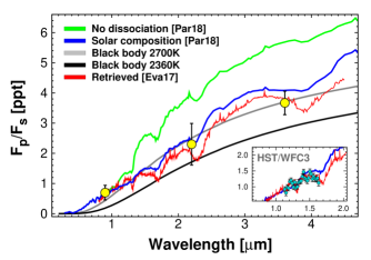
Figure 7: Comparison of the single-band secondary transit depths with the planetary atmosphere models of Parmentier et al. (parmentier2018 (2018), [Par18]) and Evans et al. (evans2017 (2017), [Eva17]). The error bars show $3\sigma$ statistical uncertainties. We warn that the “No dissociation” model is unphysical, and is shown merely to limelight the effect of omitting dissociation in the computation of the spectrum (see text for further details). The black-body lines correspond to different efficiency of the day/night heat transport (black: fully efficient; gray: no heat transport). For completeness, the inset shows the HST observations of Evans et al. (evans2017 (2017)) with their spectrum retrieval model and the solar composition model of [Par18]. For better visibility, we use $1\sigma$ error bars here.

Table 4: Secondary transit depths of WASP-121b.

Instr./Filter	$\lambda_{\rm c}$	Depth	Error	Source
TRAPPIST (z’)	0.9	0.697	0.081	Delrez et al. (delrez2016 (2016))
2MASS K	2.2	2.280	0.230	this paper
Spitzer/IRAC	3.6	3.670	0.130	Evans et al. (evans2017 (2017))

Notes:
Only single-band data are shown. – The central wavelength $\lambda_{\rm c}$ is given in $\mu$m, the depth and its $1\sigma$ statistical error are given in ppt (part per thousand).

The black body lines (gray and black) in Figure 7 show the effect of heat transport from the day-side to the night-side. Assuming zero Bond albedo in both cases, the black line displays the case of heat transport with maximum efficiency ($A_{\rm B}=0$, $\varepsilon=1.0$ – see Cowan & Agol cowan2011 (2011), Lopez-Morales & Seager lopez2007 (2007)). It is clear that all available data exclude this possibility and support circulation models that are rather inefficient, resulting in a higher day-side temperature. For WASP-121b, this temperature seems to be close to $2700$ K, corresponding to $\varepsilon=0.57$, assuming $A_{\rm B}=0$. In a comparison with the models of Evans et al. (evans2017 (2017)) – who use also the above planet temperature – we find that their ‘retrieved’ model slightly underestimates our occultation depth by $1.6\sigma$, whereas the mismatch for the black body line of $2700$ K is only $0.4\sigma$.

By scanning the planet temperature, we find that the best-fitting black body model to the three single-band data points (weighted equally) is reached when $T_{\rm p}=2652$ K. The RMS and the $\chi^{2}$ value of the residuals is $0.194$ ppt and $15.4$, respectively. All points are within $1\sigma$, except for the one at $0.9$ $\mu$m, that deviates by $3.8\sigma$. For the solar composition model of Parmentier et al. (parmentier2018 (2018)) we get $0.244$ ppt and $10.3$ for the RMS and $\chi^{2}$, respectively. These large values result from the Spitzer data, with a deviation of $3.2\sigma$ (the other two points deviate less than $0.5\sigma$). Repeating the same comparison for the retrieved model of Evans et al. (evans2017 (2017)), we get, respectively, $0.238$ ppt and $4.7$ for the RMS and $\chi^{2}$. Now all points deviates just barely under $1\sigma$, except for the $2.2$ $\mu$m point, that deviates by $1.6\sigma$.

It is important to note that the status of the outliers might change with a different way of handling systematics. As mentioned, over-correcting systematics may lead to lower occultation depth (e.g., we got larger depth from the $0.9$ $\mu$m data by $\sim 0.1$ ppt than the one derived by Delrez et al. delrez2016 (2016), quite likely, because of the lack of polynomial correction in our derivation).

With the data available today, it seems that the retrieval model of Evans et al. (evans2017 (2017)) is capable to catch most of the features of the observed spectrum. The fact that our data deviates by $1.6\sigma$ from their model spectrum, indicates that although additional fine tuning is needed, the basic characteristics of the data are well-matched. On the other hand, the required $VO$ abundance is some thousand times of the solar value, which warrants some caution (see Evans et al. evans2017 (2017) and Parmentier et al. parmentier2018 (2018) for further discussion of this issue with the emission spectrum).

Additional complications come from the more extensive data available from HST and ground-based transmission spectrum measurements. The recent analysis of these data by Evans et al. evans2018 (2018)) lends further support for a high (10–30-times solar) $VO$ abundance and lack of $TiO$. Furthermore, these data also pose some challenges in explaining the steep rise of the absorption in the near ultraviolet regime. The authors invoke sulfanyl ($SH$) as a possible absorber, since the standard explanation by Rayleigh scattering fails in the case of WASP-121b, due to the high atmospheric temperature implied by Rayleigh scattering only.

Unfortunately, the currently available data on WASP-121b still too sparsely populate the more easily measurable part of the emission spectrum. In the waveband between $2$ $\mu$m and $4$ $\mu$m (where the $CO$ and $H_{2}O$ emissions are the most pronouncing) additional data would be of great help. High S/N measurements carried out by instruments like CRIRES at VLT would be clearly capable to map this crucial region. In addition to the determination of the abundances of the molecules above, this would perhaps constrain also the abundances derived from the shorter wavelength part of the spectrum, where high S/N data gathering is more difficult.

5 Conclusions

We presented the first secondary transit measurements of an extrasolar planet in the near infrared by using a 1-m class telescope. With the ANDICAM imager attached to the $1.3$ m telescope of the SMARTS Consortium, we detected an occultation depth of $(0.228\pm 0.023)$% in the 2MASS K band from observations made in three nights on the very hot Jupiter WASP-121b. We compared this value with theoretical planetary spectra of Parmentier et al. (parmentier2018 (2018)) and Evans et al. (evans2017 (2017)) and found that it fits perfectly the former model, using solar composition, atmospheric circulation and molecular dissociation. However, when considering all available secondary transit data (Sloan z’, HST and Spitzer data – see Delrez et al. delrez2016 (2016) and Evans et al. evans2017 (2017)), it seems that the $VO$-enhanced model of Evans et al. (evans2017 (2017)) is preferred over the solar composition model, albeit with a less favorable match to our data. Although the $2700$ K black body line yields also an acceptable overall fit to the available data, the more detailed HST spectrum is not reproduced well. Additional data in the $(2$ – $4)$ $\mu$m regime would be very useful to verify model predictions on $CO$ and $H_{2}O$ emissions and build a more coherent planet atmosphere model.

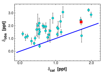
Figure 8: Observed vs calculated secondary transit depths for the $32$ extrasolar planets known today with emission measurements at $\sim 2.2$ $\mu$m. Nearly all observations lie above the equality line, corresponding to the calculated/expected black body value, assuming effective heat transport from the day side to the night side. WASP-121b is shown as a red square. Error bars show $1\sigma$ statistical errors.

In agreement with other studies (e.g., Adams & Laughlin adams2018 (2018), and references therein), our data support the lack of efficient day-to-night side heat transport (see Fig. 7). This conclusion is further strengthened if we compare the predicted and observed occultation depths by using all available data today. Based on the list of Alonso (alonso2018 (2018)), we collected the secondary transit depths measured in the 2MASS K band for $32$ Hot Jupiters (see Croll et al. croll2015 (2015), Cruz et al. cruz2015 (2015), Zhou et al. zhou2015 (2015), Martioli et al. martioli2018 (2018) and this paper). The observed depths as a function of the expected value (assuming zero Bond albedo and fully efficient heat transport) are shown in Fig. 8. The figure clearly shows a nearly uniform offset, with no apparent dependence on the expected depth. The effect is exacerbated if we consider more realistic albedos as suggested by recent analyses of full orbit phase curves – see Adams & Laughlin (adams2018 (2018)).

We arrive to a similar conclusion if we examine the difference between the observed and calculated occultation depths as a function, e.g., of the temperature at the substellar point. Therefore, – admitting the need for a more complete characterization of the heat distribution by directly measuring the night- and day-side fluxes (i.e., Komacek & Showman komacek2016 (2016)) – from the $2.2$ $\mu$m measurements alone, there does not seem to exist a correlation between the heat redistribution efficiency and planet temperature (i.e., Cowan & Agol cowan2011 (2011), Komacek & Showman komacek2016 (2016)). Supporting our result, it is interesting to note that a similar study by Baskin et al. (baskin2013 (2013)), based on Spitzer $3.6$ $\mu$m and $4.5$ $\mu$m data has led to the same conclusion.

Although our observations were made in a single waveband, they yield a reasonably solid piece of information both on the orbital and on the atmospheric characterization of the WASP-121 system. Together with future emission data in the $(2$ – $4)$ $\mu$m band they will allow to prove or deny the existence of the $CO$, $H_{2}O$ emission feature on the day side predicted by the models in this waveband.

- (1) Adams, A. D. & Laughlin, G. 2018, AJ, 156, 28
- (2) Alonso, R. 2018, Handbook of Exoplanets, ISBN 978-3-319-55332-0, id.40 (arXiv:1803.06204)
- (3) Anderson, D. R., Temple, L. Y., Nielsen, L. D. et al. 2018, submitted to MNRAS, (arXiv: 1809.04897)
- (4) Bakos, G. Á., Torres, G., Pál, A. et al. 2010, ApJ, 710, 1724
- (5) Baskin, N. J., Knutson H. A., Burrows, A., et al. 2013, ApJ, 773, 124
- (6) Cowan, N. B. & Agol, E. 2011, ApJ, 729, 54
- (7) Croll, B., Albert, L., Jayawardhana, R. et al. 2015, ApJ, 802, 28
- (8) Cruz, P., Barrado, D., Lillo-Box, J. et al. 2015, A&A, 574A, 103
- (9) Deeg, H. J. & Tingley, B. 2017, A&A, 599, A93
- (10) Delrez, L., Santerne, A., Almenara, J.-M. et al. 2016, MNRAS, 458, 4025
- (11) Deming, D., Seager, S., Richardson, L. J., & Harrington, J. 2005, Nature, 434, 740
- (12) Evans, T. M., Sing, D. K., Wakeford, H. R. et al. 2016, ApJ, 822, L4
- (13) Evans, T. M., Sing, D. K., Kataria, T. et al. 2017, Nature, 548, 58
- (14) Evans, T. M., Sing, D. K., Goyal, J. M. et al., 2018, AJ, 156, 283
- (15) Kreidberg, L., Line, M. R., Bean, J. L., et al. 2015, ApJ, 814, 66
- (16) Komacek, T. D., & Showman, A. P. 2016, ApJ, 821, 16
- (17) Lopez-Morales, M. & Seager, S. 2007, ApJ, 667, L191
- (18) Martioli, E., Colón, K. D., Angerhausen, D. 2018, MNRAS, 474, 4264
- (19) Parmentier, V., Line, M. R., Bean, J. L. et al. 2018, A&A, 617, 110
- (20) Pollacco D. L., Skillen, I., Collier Cameron, A. et al. 2006, PASP, 118, 1407
- (21) Stevenson, K. B., Harrington, J., Fortney, J. J., et al. 2012, ApJ, 754, 136
- (22) Winn, J. N. 2010, arXiv:1001.2010v5
- (23) Zhou, G., Bayliss, D. D. R., Kedziora-Chudczer, L. et al. 2015, MNRAS, 454, 3002