Uncovering predictability in the evolution of the WTI oil futures curve

Abstract

Accurately forecasting the price of oil, the world’s most actively traded commodity, is of great importance to both academics and practitioners. We contribute by proposing a functional time series based method to model and forecast oil futures. Our approach boasts a number of theoretical and practical advantages including effectively exploiting underlying process dynamics missed by classical discrete approaches. We evaluate the finite-sample performance against established benchmarks using a model confidence set test. A realistic out-of-sample exercise provides strong support for the adoption of our approach with it residing in the superior set of models in all considered instances.

Keywords: crude oil, forecasting, functional time series, futures contracts, futures markets

1 Introduction

Traditionally, statistical frameworks adopted in both the academic literature and practice address the modelling of low-frequency regularly spaced datasets. However, the recent availability of higher-resolution time series brings with it unique challenges and opportunities (Engle, 2000). Functional Time Series (FTS) is a convenient modelling and forecasting framework boasting the ability to tackle such problems. Tsay (2016) demonstrates that FTS analysis is widely applicable to many areas of big data analytics and business statistics. We take up this mantle and propose a novel exponential smoothing state space FTS framework to address a critical problem in empirical finance, namely the modelling and forecasting of crude oil futures prices.

Alquist et al. (2013) outline three critical areas for which reliable forecasts of oil prices are essential. First, airlines, automobile firms, utilities and even homeowners make pricing, consumption and investment decisions based on forecasts of oil prices. Second, oil price forecasts are a key component of central bank macroeconomic projections and market practitioners’ risk assessments, with more accurate forecasts potentially improving policy responses and risk management strategies. Third, oil price forecasts inform energy usage and carbon emission projections with regulatory policy implications such as fuel excise adjustments and climate change interventions. More specifically, in this paper, we focus on oil futures prices. In general, commodity futures are far more actively traded than their related spot contracts (see, e.g., Ng and Pirrong, 1996). Outlining the importance of futures markets, Laws and Thompson (2004) explicitly identify four functions they serve: efficient price discovery, resource allocation, risk management and financing. Furthermore, energy futures price forecasts can accurately inform the pricing of related securities and projects (Kyriakou et al., 2016).

The use of such financial derivatives in Europe has been widely documented (see, e.g., Carroll et al., 2017). More specifically for oil derivatives, Brent crude was traditionally regarded as the leading indicator of prices within Europe. However, as the United States (US) recently repealed its 40-year-old ban on exporting WTI (West Texas Intermediate) crude, forecasting WTI crude oil futures has become a vital issue for European audiences. Since the repeal of this ban, there has been a surge in WTI futures trading. This phenomenon has led to a trend of increased trading volumes for WTI oil futures coupled with reduced trading volumes for the traditionally European Brent oil futures.

Furthermore, recent production of oil in the European North Sea has seen a structural decline at a time when US WTI crude has observed record production levels. This has led to reports that the firm who set the price of Brent, S&P Global Platts, is now considering using WTI prices to calculate its latest European index. These factors have culminated in WTI arguably becoming the price discovery leader in global crude oil markets and overtaking Brent as the leading oil benchmark in Europe.

Two main classes of models are outlined in the commodity futures modelling literature: discrete latent factor and fundamental macroeconomic-based models. Latent factor approaches to model commodity futures curves include those presented by Casassus and Collin-Dufresne (2005); Chantziara and Skiadopoulos (2008); Trolle and Schwartz (2009) and Casassus et al. (2013), with a separate strand of literature concluding that fundamentals are important in explaining energy prices (see, e.g., Kilian, 2009; Singleton, 2013; Andreasson et al., 2016; Basak and Pavlova, 2016). Based on this literature we adopt the fundamental commodity futures forecasting framework of Andreasson et al. (2016), as well as the principal component approach of Chantziara and Skiadopoulos (2008) as two benchmarks for our proposed FTS model. This aligns with the approach taken by Cummins et al. (2016) who adopt both frameworks and find no discernible difference between the performance of the latent and fundamental models.

To the best of our knowledge, this paper constitutes the first application of FTS methods to describe, model and forecast commodity futures curves. In the FTS domain, the item of interest is a set of curves, shapes, objects or, more broadly, functional observations. Because trading is focused on specific segments of the oil futures curve, quotes are only observable at discrete expiry points. However, the novel approach that we propose (described in Section 3) seeks to uncover the true underlying curve dynamics that is often missed by traditional techniques. This unearthed underlying process is subsequently projected forward using an exponential smoothing model that has widespread application in business forecasting (see, e.g., Hyndman et al., 2008; Taylor, 2010). In an exponential smoothing setting, forecasts are weighted combinations of past observations–in our case, the functional principal component decomposition of daily oil futures curves. The idea is that the most recent observations inform the forecast most heavily, with weights decreasing exponentially for more distant past observations. We evaluate our forecasting models using the data snooping bias-free model confidence set (MCS) procedure of Hansen et al. (2011), as also employed by Neumann and Skiadopoulos (2013) and Baruník and Malinská (2016). Through this, we ascertain that the FTS approach is superior relative to the benchmark models.

In addition to producing more accurate one-day ahead out-of-sample oil price forecasts, the use of an FTS framework boasts several practical and conceptual advantages. First, the approach effectively captures serial dependence, a prominent attribute of daily oil futures curves. Secondly, it facilitates the modelling of data observed at a small number of unequally spaced points, as well as those with possible non-negligible measurement error, which are common in business statistics (see, e.g., Kowal et al., 2018). In our specific context, we follow Cummins et al. (2016) in focusing on the most actively traded futures contract expiries (CL1–CL9, CL12, and CL18), resulting in unequally spaced data points along the futures curve, which our FTS framework models effectively. Third, the approach facilitates the pricing of non-standard expiry OTC (over-the-counter) contracts, as the output is a complete forecasted futures curve across an essentially infinite number of expiries. Finally, and more practically, given that it relies on latent factors, our approach circumvents the need to a priori identify fundamental factors that model oil futures prices, thus mitigating the risk of omitted variable bias. The paper continues as follows: Section 2 describes the oil futures dataset, Section 3 outlines our proposed FTS methodology and forecasting evaluation framework, Section 4 presents in- and out-of-sample results and Section 5 concludes the paper.

2 Oil Futures Data

Crude oil is the world’s most heavily traded commodity futures contract (see, e.g., Sévi, 2014). More specifically, Bernardi et al. (2018) outline that WTI crude oil has the highest weighting of all futures across the three leading commodity indices compiled by Bloomberg, UBS and Dow Jones. Each WTI futures contract is written on 1,000 barrels of crude oil, whereby a price is agreed today for oil to be delivered and paid for on a specific date in the future. On any given day, a large number of contracts is traded with expiration dates in consecutive months. Generic series can be constructed by rolling from one contract to another, with CL1 representing the oil futures contract with the shortest date to expiry, CL2 the second shortest and so forth. Because of lower trading intensity, liquidity levels are reduced for certain non-standard maturities observed along the futures curve. To alleviate any such concerns, we concentrate only on the most actively traded generic monthly futures in line with Cummins et al. (2016). The futures we use are CL1–CL9, CL12 and CL18 obtained from the CME Group. The CME Group is the world’s largest marketplace for buying and selling futures contracts. It consists of four separate exchanges: the Chicago Mercantile Exchange, Chicago Board of Trade, New York Mercantile Exchange and Commodity Exchange. Our sample is at a daily frequency from January 2009 to December 2015. To construct the fundamental factor model, daily VIX quotes are downloaded from the Chicago Board of Options Exchange and S&P 500 (Standard and Poor’s 500 index) levels retrieved from Yahoo! Finance, with the Trade Weighted US Dollar Index (USD) and US Economic Policy Uncertainty Index (EcPol) both being obtained from FRED (Federal Reserve Economic Data). Descriptive statistics for our dataset are given in Table 1.

Table 1: Descriptive Statistics

	Mean	Std. Dev.	Median	Minimum	Maximum	Skewness	Kurtosis
CL1	81.51	19.99	86.72	33.98	113.93	-0.70	-0.65
CL2	82.07	19.48	87.41	35.78	114.43	-0.70	-0.66
CL3	82.50	19.00	87.94	36.79	114.71	-0.71	-0.65
CL4	82.81	18.59	88.37	37.60	114.83	-0.73	-0.62
CL5	83.05	18.20	88.77	38.45	114.82	-0.74	-0.59
CL6	83.21	17.83	89.10	39.07	114.78	-0.75	-0.55
CL7	83.31	17.50	89.36	39.68	114.73	-0.76	-0.52
CL8	83.39	17.18	89.52	40.24	114.58	-0.77	-0.48
CL9	83.44	16.88	89.56	40.88	114.38	-0.78	-0.44
CL10	83.51	16.05	89.34	42.28	113.65	-0.80	-0.33
CL11	83.32	14.59	88.21	44.41	111.71	-0.83	-0.15
VIX	20.17	8.04	17.56	10.32	56.65	1.59	2.32
S&P 500	1,481.51	390.40	1,385.14	676.53	2,130.82	0.18	-1.19
USD	77.55	6.40	75.91	68.02	94.97	1.19	0.47
EcPol	116.10	67.15	100.85	3.32	548.95	1.51	3.61

Note: This table reports the descriptive statistics of CME Group’s historical crude oil continuous futures prices. CL1 represent the next consecutive month’s futures contract, CL2 is the following month’s futures contract and so forth. The sample period is January 2009–December 2015.

Figure 1 presents plots of the relationship between oil futures prices on selected days in 2009 and 2013. In general, the spread between short- and long-expiry futures can be either positive or negative, with the relationship dependent on underlying market forces. On 30 January 2009 (Figure 1a) longer expiries are more expensive than shorter-expiry contracts, which is known as a state of contango. In Figure 1b, the opposite effect is seen, with longer-expiry futures being cheaper, which is known as backwardation. Our flexible FTS approach effectively characterises both states. Furthermore, Figure 2 presents the evolution of prices for short (1 month), medium (6 months) and long expiry (18 months) futures throughout our sample period. It can be seen that the price spread is not constant over time, with Schwartz and Smith (2000) previously establishing that such differences between short- and long-maturity contracts provide substantial information about short-term price variations. We next detail our proposed FTS framework to forecast this oil dataset.

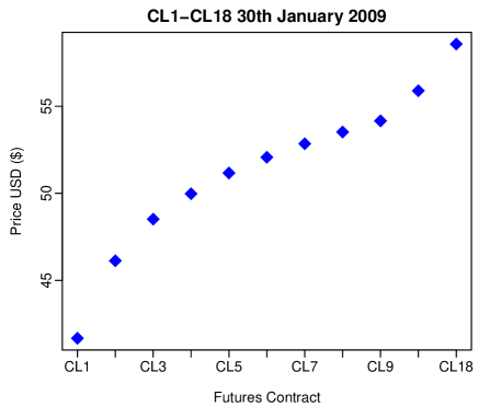
(a) Panel A

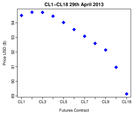
(b) Panel B

Figure 1: The crude oil continuous futures price for each of 11 different expiries on the 30 January 2009 (Panel A) and 29 April 2013 (Panel B)

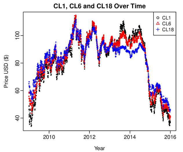
Figure 2: Evolution of three crude oil continuous futures prices over January 2009–December 2015 period; short-term, medium-term and long-term expiries are represented by CL1, CL6 and CL18, respectively

3 Methodology

3.1 Exponential Smoothing Functional Time Series Forecasts

We adopt an FTS approach to first model and subsequently forecast the relationship between the prices associated with oil futures contracts of different expiries. To model this futures curve, we first let $(\mathcal{X}_{t},t\in\mathbb{Z})$ be an arbitrary FTS defined on a common probability space $(\Omega,A,P)$. In our case $\mathcal{X}_{t}$ represents the futures curve on each day $i$, with the continuum $\theta$ given in terms of the futures contract expiry, CL1, CL2, etc. Each function is a square integrable function satisfying $\|\mathcal{X}_{t}\|^{2}=\int_{\mathcal{I}}\mathcal{X}_{t}^{2}(\theta)d\theta<\infty$. The notation $\mathcal{X}\in\mathcal{L}_{\mathcal{H}}^{p}(\Omega,A,P)$ is used to indicate that $\text{E}(\|\mathcal{X}\|^{p})<\infty$ for some $p>0$. For instance, when $p=1$, $\mathcal{X}(\theta)$ has the mean curve $\mu(\theta)=\text{E}[\mathcal{X}(\theta)]$; when $p=2$, the non-negative definite covariance function is given by

$$c_{\mathcal{X}}(\theta,\omega)=\text{Cov}[\mathcal{X}(\theta),\mathcal{X}(\omega)]=\text{E}\left\{[\mathcal{X}(\theta)-\mu(\theta)][\mathcal{X}(\omega)-\mu(\omega)]\right\},$$ (1)

for all $\theta,\omega\in\mathcal{I}$. The covariance function in (1) allows the covariance operator of $\mathcal{X}$ to be defined as:

$$\mathcal{K}_{\mathcal{X}}(\phi)(\omega)=\int_{\mathcal{I}}c_{\mathcal{X}}(\theta,\omega)\phi(\theta)d\theta.$$

There then exists an orthonormal sequence $(\phi_{k})$ of continuous functions and a non-increasing sequence $(\lambda_{k})$ of positive numbers, such that:

$$c_{\mathcal{X}}(\theta,\omega)=\sum^{\infty}_{k=1}\lambda_{k}\phi_{k}(\theta)\phi_{k}(\omega),\qquad\theta,\omega\in\mathcal{I}.$$

Therefore, a Karhunen-Loève expansion of such a stochastic process $\mathcal{X}(\theta)$ can be expressed as:

$$\mathcal{X}(\theta) =\mu(\theta)+\sum^{\infty}_{k=1}\beta_{k}\phi_{k}(\theta)$$

$$=\mu(\theta)+\sum^{K}_{k=1}\beta_{k}\phi_{k}(\theta)+e(\theta),$$ (2)

where scores $\beta_{k}$ are given by the projection of $\mathcal{X}(\theta)-\mu(\theta)$ in the direction of the $k^{\text{th}}$ eigenfunction $\phi_{k}$; that is, $\beta_{k}=\langle\mathcal{X}(\theta)-\mu(\theta),\phi_{k}(\theta)\rangle$; $e(\theta)$ denotes the model truncation error function with a mean of zero and a finite variance; and $K<n$ is the number of retained components. Equation (2) facilitates dimension reduction as the first $K$ terms often provide a good approximation to the infinite sums, and thus the information inherent in $\bm{\mathcal{X}}(\theta)$ can be adequately summarised by the $K$-dimensional vector $(\bm{\beta}_{1},\cdots,\bm{\beta}_{K})$.

There are at least four common approaches to determine our selection of $K$, namely cross-validation (Ramsay and Silverman, 2005), Akaike’s information criterion (Akaike, 1974), the bootstrap method (Hall and Vial, 2006), the ratio method (Lam and Yao, 2012) and explained variance (Chiou, 2012). Here, the value of $K$ is determined as the minimum that reaches a certain level of the proportion of total variance explained by the $K$ leading components such that:

$$K=\operatorname*{\arg\!\min}_{K:K\geq 1}\left\{\sum^{K}_{k=1}\widehat{\lambda}_{k}\Big{/}\sum^{\infty}_{k=1}\widehat{\lambda}_{k}\mathds{1}_{\left\{\widehat{\lambda}_{k}>0\right\}}\geq P_{1}\right\},$$

where $P_{1}=99\%$, $\mathds{1}_{\left\{\widehat{\lambda}_{k}>0\right\}}$ is to exclude possible zero eigenvalues, and $\mathds{1}\{\cdot\}$ represents the binary indicator function. When we align with Chantziara and Skiadopoulos (2008) and Cummins et al. (2016) and utilise three principal components, $99\%$ of the variation in our dataset is explained; therefore we also specify $P_{1}=99\%$.

By characterising the relationship between oil futures prices of different expiries in the above manner, we obtain daily functional realisations of its term structure, or futures curve. With a set of realisations $\bm{\mathcal{X}}(\theta)=\{\mathcal{X}_{1}(\theta),\dots,\mathcal{X}_{n}(\theta)\}$, the mean function can be approximated as $\widehat{\mu}(\theta)=\sum^{n}_{t=1}\mathcal{X}_{t}(\theta)/n$, and the theoretical covariance function can be empirically estimated as:

$$\widehat{c}_{n}=\frac{1}{n}\sum^{n}_{i=1}\langle\mathcal{X}_{t},x\rangle\mathcal{X}_{t},\qquad x\in\mathcal{H},$$

which is shown to be consistent under weak dependency (see, e.g., Hörmann and Kokoszka, 2010). From the empirical covariance function, we can extract estimated functional principal component functions $\bm{B}=\{\widehat{\phi}_{1}(\theta),\dots,\widehat{\phi}_{K}(\theta)\}$. Conditioning on the past functions $\bm{\mathcal{X}}(\theta)$ and the estimated functional principal components $\bm{B}$, the one-step-ahead point forecast of $\mathcal{X}_{n+1}(\theta)$ can be expressed as:

$$\widehat{\mathcal{X}}_{n+1|n}(\theta) =\text{E}[\mathcal{X}_{n+1}(\theta)|\bm{\mathcal{X}}(\theta),\bm{B}]$$

$$=\widehat{\mu}(\theta)+\sum^{K}_{k=1}\widehat{\beta}_{n+1|n,k}\widehat{\phi}_{k}(\theta),$$

where $\widehat{\beta}_{n+1|n,k}$ denotes time series forecasts of the $k^{\text{th}}$ component scores. The forecasts of these scores can be obtained via a univariate time series forecasting method, such as exponential smoothing (see Ord and Fildes, 2013, for a review), which can handle non-stationarity of the functional principal component scores.

Following early work by Gardner, Jr and McKenzie (1985), we consider a damped trend exponential smoothing model, where a parameter $0\leq\xi<1$ dampens the trend to a flat line sometime in the future. For each set of principal component scores, the resulting model is expressed as:

$$\beta_{t} =\ell_{t-1}+\xi b_{t-1}+\epsilon_{t},$$

$$\ell_{t} =\ell_{t-1}+\xi b_{t-1}+\delta\epsilon_{t},$$

$$b_{t} =\xi b_{t-1}+\gamma\epsilon_{t},$$

where $\ell_{t}$ denotes level at time $t=1,\dots,n$, $b_{t}$ denotes the growth rate and $\epsilon_{t}$ denotes the error term. Elton et al. (2006) also consider exponential smoothing for financial economic forecasting.

3.2 Benchmarks

To evaluate the performance of our proposed FTS framework, we employ the use of fundamental and latent factor benchmarks. We utilise fundamental factors proposed by Andreasson et al. (2016) to model commodity futures prices, namely the Trade Weighted US Dollar Exchange Rate, S&P 500 Index levels, the VIX (a measure of the market’s expectation of future S&P 500 index volatility) and the EcPol developed by Baker et al. (2015). The model is specified as follows:

$$\text{Oil}_{t}^{\tau}=\zeta+\beta_{1}\text{SP500}_{t-1}+\beta_{2}\text{VIX}_{t-1}+\beta_{3}\text{USD}_{t-1}+\beta_{4}\text{EcPol}_{t-1}+\varepsilon_{t},$$

with $\text{Oil}^{\tau}_{t}$ denoting the log return of the oil futures with expiry $\tau$ at time $t$, $\zeta$ denoting the intercept term, SP500_t-1 denoting S&P 500 log return at time $t-1$, VIX_t-1 denoting VIX volatility index log change at time $t-1$, USD denoting the trade-weighted US dollar index at time $t-1$, EcPol_t-1 denoting US Economic Policy Uncertainty Index log change at time $t-1$ and $\varepsilon_{t}$ denoting the error term at time $t$. We hereafter refer to this model as Fundamental.

Our second benchmark is the latent factor model, as proposed by Chantziara and Skiadopoulos (2008). They use three discrete principal component extractions as factors for forecasting, as follows:

$$\text{Oil}_{t}^{\tau}=\zeta+\beta_{1}\text{f}_{1,t-1}+\beta_{2}\text{f}_{2,t-1}+\beta_{3}\text{f}_{3,t-1}+\upsilon_{t},$$

where $\text{f}_{1,t-1},\text{f}_{2,t-1}$ and $\text{f}_{3,t-1}$ denote the first, second and third principal components calculated from the oil futures prices, $\beta_{1},\beta_{2}$ and $\beta_{3}$ denote the coefficients and $\upsilon_{t}$ denotes the error term. We hereafter refer to this model as PC.

Finally, as a naïve benchmark, we also incorporate the random walk without drift into our in-sample analysis. The random walk without drift model can be expressed as:

$$\text{Oil}_{n+1}^{\tau}=\text{Oil}_{n}^{\tau}+\nu_{n+1},$$

where $\nu_{n+1}$ is a zero-mean error term that is uncorrelated to $\text{Oil}_{n}^{\tau}$. The random walk without drift is also utilised in the out-of-sample performance evaluation to produce the Mean Absolute Scaled Error (MASE) as proposed by Hyndman and Koehler (2006). The MASE loss function is further detailed in the following sections.

3.3 Forecast Evaluation

Out-of-sample forecasts are obtained using an expanding scheme. Each day an additional observation is added to an expanding training window with the models being re-estimated. We choose to expand the training set and re-estimate the model at each time step, daily, to incorporate all available up-to-date information into our forecast. Using our January 2009–December 2015 dataset, we statistically compare the model forecasts using a 500-day out-of-sample window, whereby the January 2009–December 2013 period is initially designated as the training window with the calculated forecasts being compared with the 500 unknown observations in the December 2013–December 2015 window. As an additional robustness check that controls for sensitivity to the specific out-of-sample period, 250-day and 750-day out-of-sample windows are also specified. We evaluate in-sample predictions using (where appropriate) a variety of performance measures: Mean Absolute Error (MAE), Mean Mixed Error Under (MME(U)), Mean Mixed Error Over (MME(O)), and Mean Correct Predictor of the Direction of Change (MCPDC).

3.4 Loss Functions

We assess the performance of the models using the following measures:

1. MAE is the average of the absolute differences between the prediction, ${\textstyle\widehat{\text{Oil}}_{n+\vartheta|n+\vartheta-1}}$, and the corresponding observation, ${\text{Oil}_{n+\vartheta}}$. It measures the average error magnitude of the predictions, regardless of error direction and serves to aggregate errors into a single measure of predictive power:

   $$\text{MAE}^{\tau} =\frac{1}{T}\sum_{\vartheta=1}^{T}\left|\text{Oil}^{\tau}_{n+\vartheta}-\textstyle\widehat{\text{Oil}}^{\tau}_{n+\vartheta|n+\vartheta-1}\right|,\qquad\tau=1,\dots,11,$$

   $$\text{MAE}_{\text{overall}} =\frac{1}{11}\sum^{11}_{\tau=1}\text{MAE}^{\tau},$$

   where ${\text{Oil}^{\tau}_{n+\vartheta}}$ and ${\textstyle\widehat{\text{Oil}}^{\tau}_{n+\vartheta|n+\vartheta-1}}$ are the observed values and their predictions for a particular expiry and model, and $T$ denotes the number of observations in the forecasting period.

2. Mean error (ME) is the average of the differences between the prediction, ${\textstyle\widehat{\text{Oil}}_{n+\vartheta|n+\vartheta-1}}$, and the corresponding observation, ${\text{Oil}_{n+\vartheta}}$. It measures the average error magnitude of the predictions, taking into account error direction, and serves to aggregate errors into a single measure of predictive power:

   $$\text{ME}^{\tau} =\frac{1}{T}\sum_{\vartheta=1}^{T}\left(\text{Oil}^{\tau}_{n+\vartheta}-\textstyle\widehat{\text{Oil}}^{\tau}_{n+\vartheta|n+\vartheta-1}\right),\qquad\tau=1,\dots,11,$$

   $$\text{ME}_{\text{overall}} =\frac{1}{11}\sum^{11}_{\tau=1}\text{ME}^{\tau},$$

   where ${\text{Oil}^{\tau}_{n+\vartheta}}$ and ${\textstyle\widehat{\text{Oil}}^{\tau}_{n+\vartheta|n+\vartheta-1}}$ are the observed values and their predictions for a particular expiry and model, and $T$ denotes the number of observations in the forecasting period.

3. MASE utilises the error produced by an in-sample naïve random walk without drift to scale and compare the out-of-sample errors observed. It measures the error magnitude scaled by the magnitude of the in-sample error:

   $$q_{\vartheta}^{\tau}=\frac{\text{Oil}_{n+\vartheta}^{\tau}-\widehat{\text{Oil}}^{\tau}_{n+\vartheta|n+\vartheta-1}}{\frac{1}{n-1}\sum^{n}_{\varphi=2}|\text{Oil}_{\varphi}-\text{Oil}_{\varphi-1}|},\qquad\vartheta=1,\dots,T.$$

   The error metric is independent of the scale of the data. A scaled error is less than one if it produces a better forecast than the average one-step, naïve forecast computed in-sample (Hyndman and Koehler, 2006). The MASE is simply:

   $$\text{MASE}=\frac{1}{T\tau}\sum^{T}_{\vartheta=1}\sum^{11}_{\tau=1}\left|q_{\vartheta}^{\tau}\right|.$$

4. MME is an asymmetric loss function. MME(U) penalises under-predictions more heavily, while MME(O) penalises over-predictions more heavily. It is not a scoring rule in the conventional sense. However, it is useful in that it provides us with an indication of the tendency of a model to under- or over-predict. This is an important consideration for consumers of oil, as under-predictions of future oil prices may be of greater concern to those in need of future supply:

   $$\text{MME}^{\tau}\text{(U)} =\frac{1}{T}\left[\sum_{\psi=\eta_{1}^{\text{O}}}^{\eta_{m}^{\text{O}}}\left|\text{Oil}^{\tau}_{n+\psi}-\textstyle\widehat{\text{Oil}}^{\tau}_{n+\psi|n+\psi-1}\right|+\sum_{\psi=\eta_{1}^{\text{U}}}^{\eta_{m}^{\text{U}}}\sqrt{\left|\text{Oil}^{\tau}_{n+\psi}-\textstyle\widehat{\text{Oil}}^{\tau}_{n+\psi|n+\psi-1}\right|}\right],$$

   $$\text{MME}^{\tau}\text{(O)} =\frac{1}{T}\left[\sum_{\psi=\eta_{1}^{\text{U}}}^{\eta_{m}^{\text{U}}}\left|\text{Oil}^{\tau}_{n+\psi}-\textstyle\widehat{\text{Oil}}^{\tau}_{n+\psi|n+\psi-1}\right|+\sum_{\psi=\eta_{1}^{\text{O}}}^{\eta_{m}^{\text{O}}}\sqrt{\left|\text{Oil}^{\tau}_{n+\psi}-\textstyle\widehat{\text{Oil}}^{\tau}_{n+\psi|n+\psi-1}\right|}\right],$$

   $$\text{MME}(\text{U})_{\text{overall}} =\frac{1}{11}\sum^{11}_{\tau=1}\text{MME}^{\tau}\text{(U)},$$

   $$\text{MME}(\text{O})_{\text{overall}} =\frac{1}{11}\sum^{11}_{\tau=1}\text{MME}^{\tau}\text{(O)},$$

   where $\eta_{m}^{\text{U}}$ denotes the number of under-predictions and $\eta_{m}^{\text{O}}$ denotes the number of over-predictions. $\big{\{}\eta_{1}^{\text{O}},\dots,\eta_{m}^{\text{O}}\big{\}}$ represents the indices of the over-predictions, and $\big{\{}\eta_{1}^{\text{U}},\dots,\eta_{m}^{\text{U}}\big{\}}$ represents the indices of the under-predictions.

5. The MCPDC is the percentage of predictions for which the prediction, ${\textstyle\widehat{\text{Oil}}_{n+\vartheta|n+\vartheta-1}}$, has the same sign as the corresponding observation, ${\text{Oil}_{n+\vartheta}}$. MCPDC measures how well the model can predict the direction of movement, regardless of error magnitude.

When evaluating out-of-sample forecasts, as opposed to in-sample predictions, we refer to the above measures as Mean Absolute Forecast Error (MAFE), Mean Forecast Error (MFE), Mean Absolute Scaled Forecast Error (MASFE), Mean Mixed Forecast Error Under (MMFE(U)), Mean Mixed Forecast Error Over (MMFE(O)), and Mean Correct Forecast of the Direction of Change (MCFDC), respectively.

4 Empirical Results

4.1 In-sample modelling

We briefly outline in-sample fit before drawing inferences using measures of out-of-sample performance. First, we outline the number of principal components used. In line with Chantziara and Skiadopoulos (2008) and Cummins et al. (2016) we specify three discrete principal components to model the oil futures curve. This results in 99% of the variance in the data being explained. Therefore, in the functional context, we also seek to explain 99% of the total variation, resulting in two functional principal components being adapted for the FTS model. Interestingly, a third functional principal component contributes less than 0.1% explained variation. We model the relationship between the curves using the FTS decomposition shown in Figure 3. The first functional principal component can be interpreted as characterising the linear relationship between the contracts, with the second component addressing the need to model the curvature dynamic. Regression results from fitting the benchmark fundamental and PC models are available upon request.

Figure 3: FTS in-sample fit: the mean fitted FTS (Functional Time Series) model and a graphical representation of its FPC (Functional Principal Component) decomposition over the January 2009–December 2013 period

We now seek to establish how well the models fit in an in-sample modelling exercise. In-sample modelling results using MAE, MCPDC, MME(U) and MME(O) loss functions are presented in Table 2. Each row shows the calculated performance measure on an individual expiry basis with the Overall row presenting the loss function aggregated across all contracts. In a cross-model comparison of the absolute and asymmetric performance measures the results of the in-sample fit using our training set are broadly similar. More specifically we observe the same Overall MAE result of 0.0129 across the PC, FTS and Fundamental models. This indicates that despite being constructed using distinct approaches each model closely calibrates to the in-sample patterns present in the dataset. Furthermore, this is in line with Cummins et al. (2016) who find no discernible in-sample difference between the competing oil futures models. Interestingly, all models considered outperform the naïve random walk which led to an Overall MAE of 0.0188. Another notable result is that while all models correctly predict the direction of change better than would be achieved by chance alone (i.e., MCPDC$>0.5$), the FTS boasts the greatest overall success, at 53.38%, versus 52.70% for the Fundamental and 52.95% for the PC models.

Table 2: In-sample Loss Functions

Expiry	MAE					MCPDC
	PC	FTS	Fund	RW		PC	FTS	Fund
Overall	0.0129	0.0129	0.0129	0.0188		0.5295	0.5338	0.5270
CL1	0.0152	0.0152	0.0152	0.0220		0.5325	0.5245	0.5277
CL2	0.0144	0.0145	0.0145	0.0209		0.5398	0.5213	0.5229
CL3	0.0139	0.0139	0.0139	0.0202		0.5261	0.5277	0.5205
CL4	0.0135	0.0135	0.0135	0.0197		0.5277	0.5285	0.5213
CL5	0.0131	0.0132	0.0131	0.0192		0.5301	0.5333	0.5237
CL6	0.0128	0.0128	0.0128	0.0187		0.5333	0.5357	0.5349
CL7	0.0125	0.0125	0.0125	0.0183		0.5285	0.5373	0.5333
CL8	0.0123	0.0123	0.0123	0.0180		0.5261	0.5365	0.5309
CL9	0.0120	0.0120	0.0120	0.0176		0.5253	0.5414	0.5317
CL12	0.0114	0.0114	0.0114	0.0167		0.5245	0.5414	0.5269
CL18	0.0105	0.0105	0.0105	0.0154		0.5309	0.5446	0.5229
Expiry	MME(U)					MME(O)
	PC	FTS	Fund			PC	FTS	Fund
Overall	0.0562	0.0569	0.0562			0.0583	0.0575	0.0582
CL1	0.0628	0.0637	0.0626			0.0627	0.0618	0.0627
CL2	0.0608	0.0617	0.0609			0.0615	0.0606	0.0615
CL3	0.0592	0.0600	0.0594			0.0605	0.0597	0.0605
CL4	0.0581	0.0588	0.0583			0.0596	0.0589	0.0596
CL5	0.0570	0.0577	0.0570			0.0590	0.0583	0.0589
CL6	0.0560	0.0566	0.0560			0.0583	0.0576	0.0582
CL7	0.0550	0.0558	0.0551			0.0578	0.0571	0.0576
CL8	0.0543	0.0550	0.0543			0.0573	0.0566	0.0571
CL9	0.0536	0.0543	0.0536			0.0568	0.0561	0.0566
CL12	0.0519	0.0525	0.0519			0.0552	0.0545	0.0550
CL18	0.0493	0.0498	0.0495			0.0526	0.0519	0.0523

Note: For each of the 11 different expiry continuous crude oil futures in our sample, this table presents the calculated performance measures (MAE, MME(U/O), and MCPDC) for the FTS, Fund (Fundamental) and PC models fitted to our daily dataset during the January 2009–December 2013 in-sample period. Overall refers to the loss function aggregated across all considered expiries. RW represents the random walk without drift. Because of its construction, it is not appropriate to calculate MCPDC and MME(U/O) for RW.

4.2 Out-of-sample forecasts

To overcome the potential for in-sample data overfitting we derive inferences from our out-of-sample testing results. The out-of-sample framework aims to answer the question; how well do the models perform in terms of producing accurate forecasts of unknown future observations? We choose to employ a recursively expanding estimation window as it closely represents a situation a practitioner might find themselves in, whereby they use all available data up to today to forecast tomorrow’s price. An alternative approach is to use a rolling fixed-length estimation window. We argue, however, that our expanding window approach represents a more appropriate environment for the exponential smoothing framework to determine its weightings, given that it internally deems observations in the distant past to have less of an effect on current forecasts.

Table LABEL:tab:3 presents the loss functions produced under our out-of-sample exercise. To produce the dynamic iterative forecasts, the tsa \ package o Hyndman and Shang (2018) was employed. The FTS model shows a lower forecasted absolute error overall, with its forecasting improvement not being confined to any one segment of the futures curve. The MFE loss function also indicates that the FTS has the lowest error, both overall–at -0.0010 versus -0.0017 and -0.0016, for FTS versus PC and Fundamental, respectively–and across each of the individual contract maturities. Furthermore, the use of the MASFE measure results in a similar conclusion with an error measure of 0.7286 overall for FTS versus 0.7324 and 0.7382, for PC and Fundamental, respectively. When we focus on a purely directional loss function, the FTS model correctly predicts the direction of price change more often than PC and Fundamental, and, very importantly, more often than by chance alone (i.e., MCFDC$>0.5$) for each expiry. Analysing the asymmetric MMFE(U) and MMFE(O) loss functions shows us that the FTS model has a comparative tendency to overestimate the price change–information that might be useful for instance, when adopting such forecasting frameworks for use in hedging or trading applications. The FTS model’s comparative tendency to overestimate price changes might result in contrasting implications for those adopting it for hedging or speculative trading activities. Finally, using 250 and 750 days as alternative out-of-sample window lengths leads to qualitatively similar results being obtained.

Table 3: Out-of-sample Loss Functions

Expiry	MAFE				MCFDC
	PC	FTS	Fund		PC	FTS	Fund
Overall	0.0138	0.0137	0.0139		0.5087	0.5169	0.4831
CL1	0.0166	0.0166	0.0168		0.5480	0.5060	0.4640
CL2	0.0160	0.0160	0.0162		0.5440	0.5160	0.4640
CL3	0.0154	0.0153	0.0156		0.5020	0.5180	0.4660
CL4	0.0149	0.0148	0.0151		0.4960	0.5220	0.4820
CL5	0.0144	0.0143	0.0145		0.4960	0.5220	0.4820
CL6	0.0138	0.0137	0.0139		0.4920	0.5160	0.4860
CL7	0.0135	0.0134	0.0135		0.4960	0.5280	0.4960
CL8	0.0131	0.0130	0.0131		0.5080	0.5220	0.5020
CL9	0.0126	0.0125	0.0126		0.5020	0.5220	0.4880
CL12	0.0115	0.0115	0.0116		0.4960	0.5100	0.4920
CL18	0.0097	0.0096	0.0097		0.5160	0.5040	0.4920
Expiry	MASFE				MFE
	PC	FTS	Fund		PC	FTS	Fund
Overall	0.7324	0.7286	0.7382		-0.0017	-0.0010	-0.0016
CL1	0.7548	0.7551	0.7656		-0.0021	-0.0012	-0.0021
CL2	0.7628	0.7627	0.7737		-0.0019	-0.0011	-0.0019
CL3	0.7621	0.7587	0.7706		-0.0018	-0.0010	-0.0018
CL4	0.7575	0.7526	0.7640		-0.0018	-0.0010	-0.0017
CL5	0.7507	0.7452	0.7557		-0.0017	-0.0010	-0.0017
CL6	0.7389	0.7335	0.7424		-0.0017	-0.0010	-0.0016
CL7	0.7356	0.7290	0.7386		-0.0016	-0.0009	-0.0016
CL8	0.7267	0.7220	0.7304		-0.0016	-0.0009	-0.0015
CL9	0.7133	0.7077	0.7164		-0.0015	-0.0009	-0.0015
CL12	0.6918	0.6873	0.6939		-0.0014	-0.0008	-0.0014
CL18	0.6261	0.6228	0.6297		-0.0013	-0.0007	-0.0012
Expiry	MMFE(U)				MMFE(O)
	PC	FTS	Fund		PC	FTS	Fund
Overall	0.0646	0.0624	0.0647		0.0530	0.0549	0.0536
CL1	0.0728	0.0704	0.0733		0.0583	0.0608	0.0595
CL2	0.0710	0.0684	0.0711		0.0574	0.0598	0.0585
CL3	0.0694	0.0671	0.0698		0.0566	0.0584	0.0573
CL4	0.0682	0.0659	0.0684		0.0558	0.0574	0.0563
CL5	0.0667	0.0644	0.0668		0.0545	0.0561	0.0549
CL6	0.0649	0.0627	0.0648		0.0537	0.0555	0.0542
CL7	0.0643	0.0619	0.0641		0.0527	0.0541	0.0530
CL8	0.0628	0.0608	0.0627		0.0517	0.0533	0.0520
CL9	0.0610	0.0591	0.0612		0.0509	0.0523	0.0511
CL12	0.0579	0.0560	0.0578		0.0484	0.0502	0.0488
CL18	0.0521	0.0499	0.0518		0.0436	0.0458	0.0443

Note: For each of the 11 different expiry continuous crude oil futures in our sample, this table presents the calculated forecast performance measures (MAFE, MASFE, MFE, MMFE(U/O) and MCFDC) for the out-of-sample forecasts produced by our FTS, Fund (Fundamental) and PC frameworks during the December 2013–December 2015 period. Overall refers to the loss function aggregated across all 11 expiries. The lowest forecast errors are shown in bold.

As these measures are simply indicators of an improvement in performance, we need to establish if the FTS model is indeed statistically superior. To this end, we turn to the MCS results presented in Table 4, where model confidence sets are constructed at confidence levels of 75% and 90% in line with Hansen et al. (2011). Details of the MCS framework are presented in the Appendix. As also outlined there, absolute error is adapted to distinguish between models in terms of out-of-sample performance. From the Overall row, the FTS resides exclusively in the superior set of models across the full futures curve, and for both test statistics. Furthermore, when focusing on each of the individual futures expiries, the FTS is classified, although not always exclusively, as a superior model in each case. Our MCS approach robustly identifies model outperformance, with its design inherently controlling for multiple comparisons. Multiple comparisons is the issue that given a sufficient number of simultaneous tests seemingly significant outperformance will be uncovered by chance alone.

Table 4: Model Confidence Set Results

	$\alpha=0.25$					$\alpha=0.1$
Statistic	Expiry	PC	FTS	Fundamental		Expiry	PC	FTS	Fundamental
$T_{\text{R,M}}$	Overall		$\dagger$			Overall		$\ddagger$
	CL1	$\dagger$	$\dagger$			CL1	$\ddagger$	$\ddagger$
	CL2	$\dagger$	$\dagger$			CL2	$\ddagger$	$\ddagger$
	CL3	$\dagger$	$\dagger$			CL3	$\ddagger$	$\ddagger$
	CL4		$\dagger$			CL4	$\ddagger$	$\ddagger$
	CL5		$\dagger$			CL5	$\ddagger$	$\ddagger$
	CL6		$\dagger$			CL6	$\ddagger$	$\ddagger$
	CL7		$\dagger$			CL7		$\ddagger$
	CL8		$\dagger$			CL8	$\ddagger$	$\ddagger$
	CL9		$\dagger$			CL9	$\ddagger$	$\ddagger$
	CL12	$\dagger$	$\dagger$			CL12	$\ddagger$	$\ddagger$	$\ddagger$
	CL18	$\dagger$	$\dagger$			CL18	$\ddagger$	$\ddagger$
$T_{\text{max},\text{M}}$	Overall		$\dagger$			Overall		$\ddagger$
	CL1	$\dagger$	$\dagger$			CL1	$\ddagger$	$\ddagger$
	CL2	$\dagger$	$\dagger$			CL2	$\ddagger$	$\ddagger$
	CL3	$\dagger$	$\dagger$			CL3	$\ddagger$	$\ddagger$
	CL4		$\dagger$			CL4	$\ddagger$	$\ddagger$
	CL5		$\dagger$			CL5	$\ddagger$	$\ddagger$
	CL6		$\dagger$			CL6	$\ddagger$	$\ddagger$
	CL7		$\dagger$			CL6	$\ddagger$	$\ddagger$
	CL8		$\dagger$			CL8	$\ddagger$	$\ddagger$
	CL9		$\dagger$			CL9	$\ddagger$	$\ddagger$
	CL12	$\dagger$	$\dagger$			CL12	$\ddagger$	$\ddagger$
	CL18	$\dagger$	$\dagger$			CL18	$\ddagger$	$\ddagger$

Note: For each of the 11 different expiry continuous crude oil futures in our sample, this table presents the results of the model confidence test of Hansen et al. (2011) based on the out-of-sample forecasts produced by PC, our FTS and Fundamental methods during the December 2013–December 2015 period. Overall refers to forecasts aggregated across each of the 11 expiries: $\dagger$ and $\ddagger$ are used to indicate that the framework resides in the superior set of models at 75% and 90% confidence levels, respectively.

Table 5 presents the results from alternative forecast evaluation frameworks to show the robustness of our results to the choice of test selected. All of the pairwise tests of our proposed functional approach versus the Fundamental or PC models indicate that our FTS model outperforms at the 1% significance level. This is consistent when employing the test of predictive accuracy in Diebold and Mariano (1995), the modified version in Harvey et al. (1997) and the test of conditional predictive ability in Giacomini and White (2006). When we focus on the collective tests that simultaneously evaluate all models with respect to a reference benchmark model, we again verify that the forecast produced by the FTS model is a significant improvement over those of the other models considered. More specifically, when we specify the PC model as a benchmark, the superiority is consistent at the 1% significance level for both White’s(2000) reality check and Hansen’s(2005) superior predictive ability tests. However, when we specify the Fundamental model as the benchmark, only the Hansen (2005) test is shown to be significant. This serves to highlight the increased power of the Hansen (2005) test over the White’s(2000) reality check on which it is based. Overall, these results provide additional evidence to support the conclusion that the FTS forecasting approach is indeed significantly better than both the PC and Fundamental models.

Table 5: Alternative Statistical Tests

	Pairwise Tests			Collective Tests
Test	FTS Vs Fund	FTS Vs PC		Fund Benchmark	PC Benchmark
Diebold-Mariano (1995)	-0.0038***	-0.0096***
	(0.0030)	(0.0077)
Modified Diebold-Mariano (1997)	-8.8250***	-3.0326***
	(0.0000)	(0.0012)
White (2000) Reality Check				0.0000	0.0081***
				(0.6910)	(0.0000)
Hansen (2005) SPA				0.6365***	0.1118***
				(0.0000)	(0.0000)
Giacomini-White (2006) CPA	76.8000***	10.4300***
	(0.0000)	(0.0050)

Note: This table presents alternative tests for statistical outperformance across all the contracts considered; $p$-values associated with each test are given in parentheses beneath the calculated test statistics. *, **, ***, represent significance at the 10%, 5%, and 1% levels, respectively. The models considered are FTS, PC and Fund (Fundamental); CPA, conditional predictive ability; SPA, superior predictive ability. Please see underlying texts indicated for further technical implementation details.

5 Concluding Remarks

Despite a strong practitioner need to model and accurately forecast oil futures prices, recent academic research has been unable to establish a discernible difference between the performance of competing models. We contribute to this strand of literature through the innovative introduction of an infinite dimensional class of factors, based on exponential smoothing forecasts of functional PCs. Our functional approach has many advantages. First, it circumvents the need to explicitly identify factors that model the shape of the oil futures curve. Second, it takes advantage of information that traditional models overlook; despite only certain contracts being actively quoted and traded on any given day, there is an underlying continuous smooth process linking oil futures contracts of different expiries. Finally, it is flexible in the sense that it is data driven, leaving the potential for it to be extended to other applications.

Our focus on WTI crude oil futures is motivated by the critical role of derivatives trading in Europe, as highlighted by Carroll et al. (2017), and the growing importance of WTI crude in a European context. We present out-of-sample results that provide empirical support for the adoption of our FTS approach when forecasting WTI oil futures, with the functional model residing in the superior set of models for all considered expiries. We now outline how our results link with previous studies.

First, our in-sample results agree with Cummins et al. (2016), who highlight that an in-sample fitting indicates no discernible difference between latent and macroeconomic factors when modelling oil futures. However, our proposal to employ the FTS model in the out-of-sample context contradicts their conclusions by uncovering a statistically outperforming forecasting model. Second, the contrasting in- and out-of-sample findings suggest that instability or overfitting might be influencing forecasting evaluation. These statistical phenomena have previously been highlighted by Giacomini and Rossi (2009) and Clark (2004), respectively. Third, our results also highlight that moving beyond the discrete approaches of Chantziara and Skiadopoulos (2008) and Andreasson et al. (2016) into a continuous FTS domain yields strong empirical benefits. As well as the importance of oil price forecasts for decision making as outlined in Section 1, our uncovered forecasting outperformance could also inform economically exploitable speculative trading or hedging strategies, with their success being dependent on an individual investor’s trading costs. Future work in this area might consider alternative benchmark models and forecasting horizons, seek to construct a semi-parametric model by supplementing our FTS framework with fundamental exogenous factors, or further refine forecast accuracy through a forecast combination approach such as employed by Gao and Nardari (2018).

Appendix A: Model Confidence Set

To examine statistical significance among the three methods, we consider the Model Confidence Set (MCS). The MCS procedure proposed by Hansen et al. (2011) consists of a sequence of tests which permits to construct a set of “superior” model, where the null hypothesis of equal predictive ability (EPA) is not rejected at a certain confidence level. As the EPA test statistic can be evaluated for any loss function, we adopt the tractable absolute error measure.

The procedure begins with an initial set of models of dimension $m=3$ encompassing all the model considered, $M_{0}=\{M_{1},M_{2},M_{3}\}$. For a given confidence level, a smaller set, the superior set of models $\widehat{M}_{1-\alpha}^{*}$ is determined where $m^{*}\leq m$. The best scenario is when the final set consists of a single model, i. e., $m=1$. Let $d_{ij,t}$ denotes the loss differential between two models $i$ and $j$, that is

$$d_{ij,t}=l_{i,t}-l_{j,t},\qquad i,j=1,\dots,m,\quad t=1,\dots,n,$$

and calculate

$$d_{i\cdot,t}=\frac{1}{m-1}\sum_{j\in\text{M}}d_{ij,t},\qquad i=1,\dots,m$$

as the loss of model $i$ relative to any other model $j$ at time point $t$. The EPA hypothesis for a given set of M candidate models can be formulated in two ways:

$$\text{H}_{\text{0,M}}:c_{ij} =0,\qquad\text{for all}\quad i,j=1,2,\dots,m$$

$$\text{H}_{\text{A,M}}:c_{ij} \neq 0,\qquad\text{for some}\quad i,j=1,2,\dots,m.$$ (A.1)

or

$$\text{H}_{\text{0,M}}:c_{i.} =0,\qquad\text{for all}\quad i,j=1,2,\dots,m$$

$$\text{H}_{\text{A,M}}:c_{i.} \neq 0,\qquad\text{for some}\quad i,j=1,2,\dots,m.$$ (A.2)

where $c_{ij}=\text{E}(d_{ij})$ and $c_{i.}=\text{E}(d_{i.})$ are assumed to be finite and time independent. Based on $c_{ij}$ or $c_{i.}$, we construct two hypothesis tests as follows:

$$t_{ij}=\frac{\overline{d}_{ij}}{\sqrt{\widehat{\text{Var}}\left(\overline{d}_{ij}\right)}},\qquad t_{i.}=\frac{\overline{d}_{i.}}{\sqrt{\widehat{\text{Var}}\left(\overline{d}_{i.}\right)}},$$ (A.3)

where $\overline{d}_{i.}=\frac{1}{m-1}\sum_{j\in\text{M}}\overline{d}_{ij}$ is the sample loss of $i^{\text{th}}$ model compared to the averaged loss across models in the set $M$, and $\overline{d}_{ij}=\frac{1}{n}\sum^{n}_{t=1}d_{ij,t}$ measures the relative sample loss between the $i^{\text{th}}$ and $j^{\text{th}}$ models. Note that $\widehat{\text{Var}}\left(\overline{d}_{i.}\right)$ and $\widehat{\text{Var}}\left(\overline{d}_{ij}\right)$ are the bootstrapped estimates of $\text{Var}\left(\overline{d}_{i.}\right)$ and $\text{Var}\left(\overline{d}_{ij}\right)$, respectively. According to Hansen et al. (2011) and Bernardi and Catania (2015), we perform a block bootstrap procedure with 5,000 bootstrap samples, where the block length $p$ is given by the maximum number of significant parameters obtained by fitting an AR($p$) process on all the $d_{ij}$ term. For both hypotheses in (A.1) and (A.2), there exist two test statistics:

$$T_{\text{R,M}}=\max_{i,j\in\text{M}}|t_{ij}|,\qquad T_{\max,\text{M}}=\max_{i\in\text{M}}t_{i},$$ (A.4)

where $t_{ij}$ and $t_{i.}$ are defined in (A.3).

The MCS procedure is a sequential testing procedure, which eliminates the worst model at each step until the hypothesis of equal predictive ability is accepted for all the models belonging to a set of superior models. The selection of the worst model is determined by an elimination rule that is consistent with the test statistic,

$$e_{\text{R,M}}=\operatorname*{arg\,max}_{i\in M}\left\{\sup_{j\in M}\frac{\overline{d}_{ij}}{\sqrt{\widehat{\text{Var}}\left(\overline{d}_{ij}\right)}}\right\},\qquad e_{\max,\text{M}}=\operatorname*{arg\,max}_{i\in M}\frac{\overline{d}_{i.}}{\widehat{\text{Var}}\left(\overline{d}_{i.}\right)}.$$

To summarise, the MCS procedure to obtain a superior set of models consists of the following steps:

1. Set $M=M_{0}$;

2. If the null hypothesis is accepted, then $M^{*}=M$; otherwise use the elimination rules defined in (A.4) to determine the worst model;

3. Remove the worst model, and go to Step 2).

References

- (1)
- Akaike (1974) Akaike, H. (1974), ‘A new look at the statistical model identification’, IEEE Transactions on Automatic Control 19(6), 716–723.
- Alquist et al. (2013) Alquist, R., Kilian, L. and Vigfusson, R. J. (2013), Forecasting the price of oil, in G. Elliott, C. Granger and A. Timmermann, eds, ‘Handbook of Economic Forecasting’, Vol. 2, North-Holland: Amsterdam, The Netherlands, chapter 8, pp. 427–507.
- Andreasson et al. (2016) Andreasson, P., Bekiros, S., Nguyen, D. K. and Uddin, G. S. (2016), ‘Impact of speculation and economic uncertainty on commodity markets’, International Review of Financial Analysis 43, 115–127.
-
Baker et al. (2015)
Baker, S. R., Bloom, N. and Davis, S. J. (2015), Measuring economic policy uncertainty, Working paper
21633, National Bureau of Economic Research.
http://www.policyuncertainty.com/media/BakerBloomDavis.pdf - Baruník and Malinská (2016) Baruník, J. and Malinská, B. (2016), ‘Forecasting the term structure of crude oil futures prices with neural networks’, Applied Energy 164, 366–379.
- Basak and Pavlova (2016) Basak, S. and Pavlova, A. (2016), ‘A model of financialization of commodities’, The Journal of Finance 71(4), 1511–1556.
-
Bernardi and Catania (2015)
Bernardi, M. and Catania, L. (2015),
The model confidence set package for R, Working paper 362, University of
Rome “Tor Vergata”.
ftp://www.ceistorvergata.it/repec/rpaper/RP362.pdf - Bernardi et al. (2018) Bernardi, S., Leippold, M. and Lohre, H. (2018), ‘Maximum diversification strategies along commodity risk factors’, European Financial Management 24(1), 53–78.
- Carroll et al. (2017) Carroll, A., O’Brien, F. and Ryan, J. (2017), ‘An examination of European firms’ derivatives usage: the importance of model selection’, European Financial Management 23(4), 648–690.
- Casassus and Collin-Dufresne (2005) Casassus, J. and Collin-Dufresne, P. (2005), ‘Stochastic convenience yield implied from commodity futures and interest rates’, The Journal of Finance 60(5), 2283–2331.
- Casassus et al. (2013) Casassus, J., Liu, P. and Tang, K. (2013), ‘Economic linkages, relative scarcity, and commodity futures returns’, Review of Financial Studies 26(5), 1324–1362.
- Chantziara and Skiadopoulos (2008) Chantziara, T. and Skiadopoulos, G. (2008), ‘Can the dynamics of the term structure of petroleum futures be forecasted? Evidence from major markets’, Energy Economics 30(3), 962–985.
- Chen and Li (2017) Chen, Y. and Li, B. (2017), ‘An adaptive functional autoregressive forecast model to predict electricity price curves’, Journal of Business & Economic Statistics 35(3), 371–388.
- Chiou (2012) Chiou, J.-M. (2012), ‘Dynamical functional prediction and classification with application to traffic flow prediction’, The Annals of Applied Statistics 6(4), 1588–1614.
- Clark (2004) Clark, T. E. (2004), ‘Can out-of-sample forecast comparisons help prevent overfitting?’, Journal of forecasting 23(2), 115–139.
- Cummins et al. (2016) Cummins, M., Dowling, M. and Kearney, F. (2016), ‘Oil market modelling: A comparative analysis of fundamental and latent factor approaches’, International Review of Financial Analysis 46, 211–218.
- Diebold and Mariano (1995) Diebold, F. X. and Mariano, R. S. (1995), ‘Comparing predictive accuracy’, Journal of Business & Economic Statistics pp. 253–263.
- Elton et al. (2006) Elton, E. J., Gruber, M. J. and Spitzer, J. (2006), ‘Improved estimates of correlation coefficients and their impact on optimum portfolios’, European Financial Management 12(3), 303–318.
- Engle (2000) Engle, R. F. (2000), ‘The econometrics of ultra-high-frequency data’, Econometrica 68(1), 1–22.
- Gao and Nardari (2018) Gao, X. and Nardari, F. (2018), ‘Do commodities add economic value in asset allocation? new evidence from time-varying moments’, Journal of Financial and Quantitative Analysis 53(1), 365–393.
- Gardner, Jr and McKenzie (1985) Gardner, Jr, E. S. and McKenzie, E. (1985), ‘Forecasting trends in time series’, Management Science 31(10), 1237–1246.
- Giacomini and Rossi (2009) Giacomini, R. and Rossi, B. (2009), ‘Detecting and predicting forecast breakdowns’, The Review of Economic Studies 76(2), 669–705.
- Giacomini and White (2006) Giacomini, R. and White, H. (2006), ‘Tests of conditional predictive ability’, Econometrica 74(6), 1545–1578.
- Hall and Vial (2006) Hall, P. and Vial, C. (2006), ‘Assessing the finite dimensionality of functional data’, Journal of the Royal Statistical Society (Series B) 68(4), 689–705.
- Hansen (2005) Hansen, P. R. (2005), ‘A test for superior predictive ability’, Journal of Business & Economic Statistics 23(4), 365–380.
- Hansen et al. (2011) Hansen, P. R., Lunde, A. and Nason, J. M. (2011), ‘The model confidence set’, Econometrica 79(2), 453–497.
- Harvey et al. (1997) Harvey, D., Leybourne, S. and Newbold, P. (1997), ‘Testing the equality of prediction mean squared errors’, International Journal of Forecasting 13(2), 281–291.
- Hörmann and Kokoszka (2010) Hörmann, S. and Kokoszka, P. (2010), ‘Weakly dependent functional data’, The Annals of Statistics 38(3), 1845–1884.
- Horváth et al. (2014) Horváth, L., Kokoszka, P. and Rice, G. (2014), ‘Testing stationarity of functional time series’, Journal of Econometrics 179(1), 66–82.
- Horváth and Rice (2015) Horváth, L. and Rice, G. (2015), ‘Testing for independence between functional time series’, Journal of Econometrics 189(2), 371–382.
- Hyndman and Koehler (2006) Hyndman, R. J. and Koehler, A. B. (2006), ‘Another look at measures of forecast accuracy’, International Journal of Forecasting 22(4), 679 – 688.
-
Hyndman and Shang (2018)
Hyndman, R. J. and Shang, H. L. (2018), ftsa: Functional Time Series Analysis. R package
version 5.2.
https://CRAN.R-project.org/package=ftsa - Hyndman et al. (2008) Hyndman, R., Koehler, A. B., Ord, J. K. and Snyder, R. D. (2008), Forecasting with Exponential Smoothing: the State Space Approach, Springer Science & Business Media, Heidelberg.
- Kearney et al. (2018) Kearney, F., Cummins, M. and Murphy, F. (2018), ‘Forecasting implied volatility in foreign exchange markets: A functional time series approach’, The European Journal of Finance 24(1), 1–18.
- Kearney et al. (2015) Kearney, F., Murphy, F. and Cummins, M. (2015), ‘An analysis of implied volatility jump dynamics: Novel functional data representation in crude oil markets’, The North American Journal of Economics and Finance 33, 199–216.
- Kilian (2009) Kilian, L. (2009), ‘Not all oil price shocks are alike: Disentangling demand and supply shocks in the crude oil market’, American Economic Review 99(3), 1053–1069.
- Kokoszka et al. (2018) Kokoszka, P., Miao, H., Reimherr, M. and Taoufik, B. (2018), ‘Dynamic functional regression with application to the cross-section of returns’, Journal of Financial Econometrics 16(3), 461–485.
- Kokoszka et al. (2015) Kokoszka, P., Miao, H. and Zhang, X. (2015), ‘Functional dynamic factor model for intraday price curves’, Journal of Financial Econometrics 13(2), 456–477.
- Kowal et al. (2017) Kowal, D. R., Matteson, D. S. and Ruppert, D. (2017), ‘A Bayesian multivariate functional dynamic linear model’, Journal of the American Statistical Association 112(518), 733–744.
- Kowal et al. (2018) Kowal, D. R., Matteson, D. S. and Ruppert, D. (2018), ‘Functional autoregression for sparsely sampled data’, Journal of Business & Economic Statistics forthcoming.
- Kyriakou et al. (2016) Kyriakou, I., Nomikos, N. K., Papapostolou, N. C. and Pouliasis, P. K. (2016), ‘Affine-structure models and the pricing of energy commodity derivatives’, European Financial Management 22(5), 853–881.
- Lam and Yao (2012) Lam, C. and Yao, Q. (2012), ‘Factor modelling for high-dimensional time series: Inference for the number of ffactor’, The Annals of Statistics 40(2), 694–726.
- Laukaitis (2008) Laukaitis, A. (2008), ‘Functional data analysis for cash flow and transactions intensity continuous-time prediction using Hilbert-valued autoregressive processes’, European Journal of Operational Research 185(3), 1607–1614.
- Laws and Thompson (2004) Laws, J. and Thompson, J. (2004), ‘The efficiency of financial futures markets: Tests of prediction accuracy’, European Journal of Operational Research 155(2), 284–298.
- Liu et al. (2016) Liu, X., Xiao, H. and Chen, R. (2016), ‘Convolutional autoregressive models for functional time series’, Journal of Econometrics 194(2), 263–282.
- Müller et al. (2011) Müller, H.-G., Sen, R. and Stadtmüller, U. (2011), ‘Functional data analysis for volatility’, Journal of Econometrics 165(2), 233–245.
- Neumann and Skiadopoulos (2013) Neumann, M. and Skiadopoulos, G. (2013), ‘Predictable dynamics in higher-order risk-neutral moments: Evidence from the s&p 500 options’, Journal of Financial and Quantitative Analysis 48(3), 947–977.
- Ng and Pirrong (1996) Ng, V. K. and Pirrong, S. C. (1996), ‘Price dynamics in refined petroleum spot and futures markets’, Journal of Empirical Finance 2(4), 359 – 388.
- Ord and Fildes (2013) Ord, K. and Fildes, R. (2013), Principles of Business Forecasting, Cengage Learning, Mason, OH, USA.
- Ramsay and Silverman (2005) Ramsay, J. and Silverman, B. (2005), Functional Data Analysis, 2nd edn, Springer Series in Statistics, New York.
- Schwartz and Smith (2000) Schwartz, E. and Smith, J. E. (2000), ‘Short-term variations and long-term dynamics in commodity prices’, Management Science 46(7), 893–911.
- Sévi (2014) Sévi, B. (2014), ‘Forecasting the volatility of crude oil futures using intraday data’, European Journal of Operational Research 235(3), 643–659.
- Singleton (2013) Singleton, K. J. (2013), ‘Investor flows and the 2008 boom/bust in oil prices’, Management Science 60(2), 300–318.
- Taylor (2010) Taylor, J. W. (2010), ‘Triple seasonal methods for short-term electricity demand forecasting’, European Journal of Operational Research 204(1), 139–152.
- Trolle and Schwartz (2009) Trolle, A. B. and Schwartz, E. S. (2009), ‘Unspanned stochastic volatility and the pricing of commodity derivatives’, Review of Financial Studies 22(11), 4423–4461.
- Tsay (2016) Tsay, R. S. (2016), ‘Some methods for analyzing big dependent data’, Journal of Business & Economic Statistics 34(4), 673–688.
- Wang et al. (2008) Wang, S., Jank, W. and Shmueli, G. (2008), ‘Explaining and forecasting online auction prices and their dynamics using functional data analysis’, Journal of Business & Economic Statistics 26(2), 144–160.
- White (2000) White, H. (2000), ‘A reality check for data snooping’, Econometrica 68(5), 1097–1126.
- Zhang (2016) Zhang, X. (2016), ‘White noise testing and model diagnostic checking for functional time series’, Journal of Econometrics 194(1), 76–95.