Evidence of Outflow Induced Soft Lags of Galactic Black Holes

Abstract

The nature of lag variation of Galactic black holes remains enigmatic mostly because of nonlinear and non-local physical mechanisms which contribute to the lag of the photons coming from the region close to the central black holes. One of the widely accepted major sources of the hard lag is the inverse Comptonization mechanism. However, exact reason or reasons for soft lags is yet to be identified. In this paper, we report a possible correlation between radio intensities of several outbursting Galactic black hole candidates and amounts of soft lag. The correlation suggests that the presence of major outflows or jets also change the disk morphology along the line of sight of the observer which produces soft lags.

1 Introduction

X-ray lags of Galactic black hole candidates (hereafter GBHs) are reported in the literature Miyamoto et al. (1988) for quite some time. Lags are obtained using cross Fourier spectrum of X-ray light curves having various energy bands. The reference or soft band are selected based on the lower cutoff of the detector and on the specificity of the object needed to be studied. For RXTE, the soft band 2-5 keV is a good choice to study the GBHs as the Keplerian disk flux (Shakura & Sunyaev (1973)) maximizes within $0.1-10$ keV. Harder photons, energized via inverse Compton process (Sunyaev & Titarchuk (1980)), in the energy bands 5-10, 10-18 keV and more, are used to create cross correlate with the soft band to generate phase lag spectra. Depending on the sign of the lag integrated over the a particular frequency range, one can infers the arrival time delay between either of the two bands. Hard lags or positive lags occur when hard photons arrive later than their softer counterpart. The reverse is true for soft lags (please see Fabian et al. (2009) and Uttley et al. (2014) for details on lags related to black holes). It is believed that inverse Comptonization always produces hard lags (Payne (1980)). However, GBHs exhibit complex lag behavior which are very difficult to interpret within the standard framework. It was understood that the lags are originated due to the accretion flows.

The accretion disks around GBHs are formed due to the matter supplied from its binary companion. The companion star can supply matter via Roche Lobe overflow, tidal disruption event or winds. During the accretion, the matter gains kinetic energy by falling into deeper gravitational potential well of a black hole. The process heats up the matter which finally leads to the radiations in the entire EM spectra. The observed spectra of black hole binaries in X-ray regime contains two major components. Thermal black body part which is believed to be originated from Keplerian disk (Shakura & Sunyaev (1973)) and a power law part (Sunyaev & Titarchuk (1980)) generated due to inverse Comptonization of the soft photons inside a hot corona or Compton cloud. The origin and configuration of this so called Compton cloud remained mischievous until the mid to late 90’s. Several models like TCAF (Chakrabarti & Titarchuk, 1995), ADAF (Narayan & Yi, 1994), RIAFs (Yuan et al., 2003) are proposed to explain the spectral properties. Previous to that, Chakrabarti (1990) elaborately presented the mass independent analytical solutions of accretion flow properties around black holes. The transonic solution clearly favored the shock transition as the flow can enter into a higher entropy branch during its course towards the black hole. Due to this sudden velocity change, the sub-keplerian matter heats up more which creates the Compton cloud. The shock transition radius or shock location ($X_{s}$) depends on the angular momentum and energy of the matter at outer boundary. In order to understand the progress of Low Frequency QPOs during rising and declining phase of any outburst, one may also consider advective flow models proposed by Chakrabarti & Titarchuk (1995); Esin et al. (1997) or Blanford & Begelman (1999). Most of the advective flow models predict a variable Compton cloud which often produced by the shock formation near the centrifugal barrier Chakrabarti (1999). Numerical simulations performed by Molteni et al. (1994) indicated that the luminosity variation due to shock oscillation could result in the formations of LFQPO. Another school of thought presented numerical simulations (Fragile & Anninos (2005); Fragile et al. (2007) and Ingram et al. (2009)) which support the claim on possible origin of LFQPOs due to Lense-Thirring precision of disk plane with axis of rotation of the central black hole. However, formation of LFQPOs by Lense-Thirring precision in presence of viscosity and radiative cooling for relatively larger ($50~{}r_{g}$) Compton cloud, are yet to be tested.

Several (Cui, Chen & Zhang (1999); Nowak, Wilms & Dove (1999); Poutanen & Fabian (1999); Kara et al. (2013); Dutta & Chakrabarti (2016) (hereafter DC16), Chatterjee et al. (2017b) (hereafter CCG17b)) attempts were made to understand the X-ray lag spectra in presence of Comptonization, reflection and magnetic field and gravitational focusing. DC16 pointed out that the soft lags are seen in high inclination angle ($\theta_{obs}\geq 60^{\circ}$) sources. It was found that above a certain QPO frequency ($\nu_{tr}$), the lag changes sign from hard to soft. Coupled with Ray-Tracing (Chatterjee, Chakrabarti & Ghosh (2017a), hereafter CCG17a) and Monte-Carlo simulations, CCG17b showed the energy dependent lag variations as a function of the size of the Compton cloud, accretion rate and inclination angle. Effects of inclination angle (see CCG17a for further details) on lag magnitude were demonstrated as well. Inverse Comptonized photons naturally lag behind soft photons that are coming directly to the observer. With increasing inclination, number of reflected photons by disk increases (see CCG17a) also. The simulations by CCG17a showed a similar lag variation as were observed by DC16 in case of GX 339-4. van den Eijnden et al. (2017) performed a survey over 15 GBHs and also found that the soft lags were seen only in case of high $\theta_{obs}$ candidates. They argued that the soft lags computed for type-C QPOs are originated by the Lense-Thirring precision of the inner disk in cases of the high inclination angle Galactic black holes.

In this picture, origin of type-B QPOs differs from type-C QPOs. B-type QPOs are considered to be originated from jets (van den Eijnden et al., 2017) as the amplitude of such QPOs decreases with increasing inclination angle. It is also worthwhile to note that the LFQPOs also change their types (A, B or C), centroid frequency ($0.01\mathrm{Hz}\leq\nu_{c}\leq 20~{}\mathrm{Hz}$), amplitude and rms as an outburst progresses and very few are observed at highest/softest possible state where the effect of thermal Comptonization is found to be the least.

Table 1: Details of Source Information and Observation

Information	XTE 1550-564	XTE 1859+226	H 1743-322	GRS 1915+105
Distance (kpc)	$4.4\pm 0.5$	$8\pm 3$	$10.4\pm 2.9$	$8.6\pm 2.0$
Mass ($M_{BH}/M_{\odot}$)	$10.4\pm 2.3$	$10.8\pm 4.7$	$11.4\pm 0.9$	$12.4\pm 2.0$
Inclination (degrees)	$67\pm 10.0$	$74\pm 4.0$	$69\pm 3.0$	$70\pm 2.0$
Outburst Year	1998	1999	2003	1996
MJD span	$51065-51092$	$51464-51480$	$52730-52800$	$50350-50600$
Number of radio	12 (843 MHz), 7 (8.6 GHz)	11 (8.4 GHz)	28 (8.4 GHz)	35 (8.4 GHz)
Observation				51 (15.2 GHz)
Radio Telescope	MOST†, ATCA‡	VLA	VLA	GBI⋆, Ryle⋆
Project Code		AH0669	AL0586, AR0508,AS0762
			AJ0302, AB1075,AR0523
			AM0773, AM0759
X-Ray Observation	16	65	31	72
(RXTE PCA)
References	1, 5, 6	1, 2	1, 3	1, 4, 7

1. Tatarenko et al. (2016) and references therein; 2. Coriat et al. (2011); 3. Corbel et al. (2005); 4. Reid et al. (2014);
5. Wu et al. (2002)^†; 6. Hannikainen et al. (2001)^‡; 7. Muno et al. (2001)^⋆.

As a natural consequence of accretion, commonly, advective flow models produce significant amount of outflows. In presence of magnetic field (Lovelace, 1976), to some extent, these outflows may also be collimated into compact or blobby jets depending on the spectral state (Fender et al. (2004); Fender et al. (2009)) of the outbursting candidate. In recent years, the correlations between X-ray flux ($F^{X}$) and radio flux ($F^{R}$) for numerous black hole candidates (Merloni et al. (2003); Hannikainen et al. (1998); Corbel et al. (2003), Cadolle Bel et al. (2007), Soleri & Fender (2011); Coriat et al. (2011); Jonker et al. (2012) and Islam & Zdziarski (2018)) suggested a strong radiative and morphological connection between X-ray emitting accretion disk and synchrotron dominated radio jets.

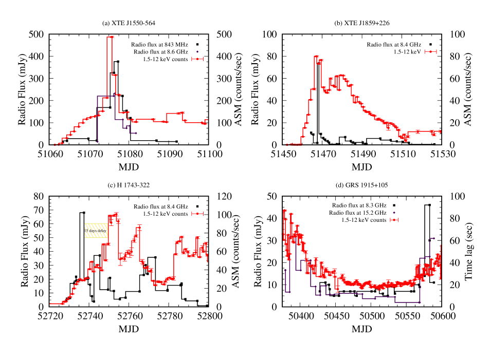
Figure 1: Radio flux and ASM counts (2-10 keV) are plotted for four candidates. In Fig. (a) and (b), we see the radio peaks are matching with the ASM maxima. In case of Fig. (c), a delay between radio and X-ray can be noticed (see §3.3 for further details). For GRS 1915+105, in between MJD 50350 to 50600, the radio flux has increased substantially in a coherent manner with the X-ray counts.

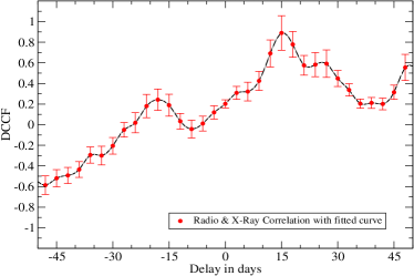
Figure 3: Discrete Cross Correlation Function (DCCF) is plotted for the radio and X-ray light curves presented in Fig. 1c. DCCF maximizes on 15 days suggesting an X-ray delay.

It is evident that the outflows/jets somehow contribute to the observed quantities like total flux and QPO frequency. Thus, to be able to understand the disk-jet connection and its implication on QPO formation, one needs to have simultaneous multi-wavelength observations. In the last decade, a few efforts were made to acquire a deeper understanding of physical mechanisms around the jet base by connecting radio, optical, and X-ray bands. Gandhi et al. (2008) showed the optical lag of GX-339-4 with respect to the X-rays and invoked a possibility of the lag to be originated by modulation of magnetic fields near the jet base. Following that, Vincentelli et al. (2018) investigated IR to X-ray lags of GX 339-4. However, the radiative coupling between disk and jet which may have affected the sub-second IR to X-ray lag remained inconclusive from their study. Later, in 2015, V 404 Cygni had undergone an outburst and was well observed in wide band. Tetarenko et al. (2019) claimed that the jet behavior changed from blobby ejecta to more compact in nature in the later stages of the outburst. The synchrotron break frequency of this object was found to be $\sim 2-5\times 10^{14}$ Hz which is in the NIR-optical band. Due to the very high break frequency, Tetarenko et al. (2019) also argued that a large fraction of photons originated in the jet region might have inverse Comptonized in the hot corona and contribute in the observed X-ray. The positive lag (soft/negative lag in our nomenclature as the lesser of the two frequency bands is lagging) of $\sim 12$ minutes between 26 and 5 GHz indicates light crossing time of $1.5$ AU. But, the absence of any such lag in between 26 and 7 GHz bands complicates the scenario more. Although their work revealed a great deal of information on the 2015 outburst of V404 Cygni, it did not probe the inner regions of jet base using X-ray timing properties. Altamirano & Méndez (2015) analyzed several outbursts of a popular black hole binary GX 339-4. The trail of hardness-phase lag followed a similar pattern to that of Cyg X-1 as they both belong to intermediate inclination $30^{\circ}<\theta_{obs}<50^{\circ}$ angle group. The soft photons (2-5 keV) for GBHs are majorly generated by the Keplerian disk and viscous time scale of such disk is believed to be in the order of few days. So, variabilities found in sub-second regime are well known to be originated by the variations of corona or Compton cloud (for further details please see Chakrabarti & Manickam (2000)). But, it is intriguing to find the average lags, even in mHz domain, are dominated by the corona and jet. Veledina et al. (2017) and Malzac et al. (2018) tried to model lag spectra between optical and X-ray using jet models. A more recent correlation between time lags and photon-index was reported by Reig et al. (2018). The correlation remains steady for rising state of low and intermediate inclination angle candidates but changes the slope for high inclination group (Fig. 3, Reig & Kylafis (2019)) and finally inverts after photon index reaches 2.0. Unlike Cyg X-1, the high inclination angle GBHs have shown negative/soft lag in X-ray band. So, the correlation might indicate about the change of lag values due to spectral state change, but, does not address how the morphology of disk-jet system might have generated the soft lags. Reig & Kylafis (2019) further investigated the lag-photon index correlation using simple jet model where optical depth of the corona/jet base falls off with increasing size of the jet base. The simulated data fits observational data of low and intermediate inclination group well. But, the jet model alone used in their simulation might not be adequate to simulate soft lags. So, under these situation, the disk-jet connection can not be ignored to understand the lag behavior of black hole candidates.

Muno et al. (2001) first reported that the lag sign changes in presence of higher activity in radio waves in GRS 1915+105. However, no follow-up observation or correlation was established to conclusively add outflows among the contributors of soft lag. More recently, CCG17b first pointed out the possibility of such correlation between time lag and radio flux seen in case of XTE J1550-564 in its 1998 outburst. In the present article, we conduct a study on four GBHs where the correlations between radio fluxes and soft lags are investigated.

This article is structured in the following way: the next Section deals with the observations and data analysis. In §3, we examine results of each candidate along with a brief description of each source. Simulated energy dependent time lags in presence of outflows are discussed in §4. We discuss possible physical explanations to corroborate observational results in §5. In §6, we draw our concluding remarks.

2 Observation and Data Analysis

We chose these four candidates (see Table 1 for details) for the availability of simultaneous radio and X-ray archival and published data. All of the four candidates have similar masses. Thus, the light crossing delay for all the sources are nearly same iff the disk size remained similar. Soft lags are mostly seen for candidates where inclination angle is high ($60^{\circ}<\theta<80^{\circ}$). The chosen candidates satisfy all of the above conditions.

2.1 Radio Data

We have used available archival Karl G. Jansky Very Large Array (VLA) data for our study. VLA has twenty seven fully steerable antennas of 25 diameter each, arranged in a ‘Y’ shaped array. Antenna configurations depend on scientific goals. The most expanded configuration is known as the ‘A’ configuration and the most compact one is called the ‘D’ configuration. ‘B’ and ‘C’ configurations are intermediate. Occasionally antennas are placed in a hybrid configurations, like ‘AB’, ‘BC’ or ‘CD’ when some of the antennas are in one configuration and some of them are in another. The maximum size of the baselines $B_{\mathrm{max}}$ in A, B, C and D configurations are 36.4, 11.1, 3.4 and 1.03 km respectively. For XTE 1859+226, the antenna were in AB configuration. The antenna were in A and D configuration for seven and twenty one days respectively for H1743–322. Here, we are only concerned about the integrated flux density of the object. So VLA configuration has no effect on the result.

Analysis and imaging of the data was carried out with Astronomical Image Processing System AIPS. The archival VLA data was read in AIPS using the task FILLM. After checking the data, we have flagged out the bad data using the task SPFLG. Then the task SETJY is used for providing the necessary source information. We have determined the calibration of the data using the task CALIB. We use the task GETJY to determine source flux densities. We used the flux density scale of Perley & Butler (2013). After that, the task CLCAL was used to apply the calibration solutions to the data. Ten seconds of integration time was used for solving amplitude and phase calibration. For the imaging and cleaning, we have used the task IMAGR and make the final image of target source. The flux density is calculated using the task JMFIT using the results of fitting a Gaussian, along with a background level. More details about the VLA data reduction can be found in the VLA cookbook.

For XTE 1550-564, we have used the published radio flux at 843 MHz from MOST radio telescope by Wu et al. (2002) and 8.6 GHz from ATCA by Hannikainen et al. (2001). We have also used the published radio flux at 8.3 GHz and 15.2 GHz for the source GRS 1915+105 from Green Bank Interferometer Monitoring Observations and Ryle radio telescope respectively by Muno et al. (2001).

2.2 X-Ray Data

We have produced time lag spectra for each observation using RXTE PCA archival data. The cross spectrum is calculated using $CF(j)=f_{1}^{*}(j)\times f_{2}(j)$, where $f_{1}$ and $f_{2}$ are the complex Fourier coefficients for the two energy bands at a frequency $\nu_{j}$. Here $f_{1}^{*}(j)$ is the complex conjugate of $f_{1}(j)$ (van der Klis et al., 1987). The phase lag between two band signals at a Fourier frequency $\nu_{j}$ is given by $\phi_{j}=arg[CF(j)]$ and the corresponding time lag is $\phi_{j}/{2\pi\nu_{j}}$ (Uttley et al., 2014). We calculated an average cross vector $CF$ by averaging complex values over multiple adjacent 16s cross spectra and then finding the final value of time lag versus frequency. We calculate time lags at the QPO centroid frequency ($\nu_{c}$) averaging over the interval $\nu_{c}\pm FWHM$ for 5-13 keV energy band against 2-5 keV energy band. For all cases of lag spectra, positive lag values mean that hard photons are lagging behind soft photons. We found that dead time effects are negligible and have ignored all the lag data where the error bar is more that $20\%$ of the time lag value. Current article contains only the lag properties of Low Frequency QPOs (type-A, type-B and type-C, see Motta et al. (2015) for further details) within the frequency range of $0.01-15.0$ Hz.

3 Results

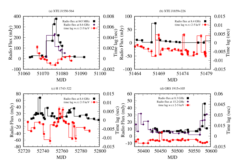
Figure 2: (a) Radio flux and X-ray soft lag shows perfect correlation for XTE J155-564. Observed radio maxima (in 8.6 GHz) coincides with soft lag maxima. (b) Radio flux and X-ray soft lag correlation for XTE J1859+226 is shown. Hard lags are only found during radio quite states. (c) Radio flux and X-ray soft lag correlation for H 1743-322 is presented. 15 days are subtracted from the original X-ray data as radio leads X-ray for H 1743-322. (d) Radio flux and X-ray soft lag correlation is shown for GRS 1915+105. Error bars, in some cases are smaller than the point size.

3.1 XTE J1550-564

XTE J1550-564 was discovered by RXTE ASM (Smith, 1998). The ASM count of the outburst achieved its peak on MJD 51076. The radio (Campbell-Wilson et al. (1998)) and optical (Orosz, Bailyn, & Jain (1998)) counterparts of this Galactic transient were detected shortly after that. Radio flux at 843 MHz (Wu et al., 2002) peaked roughly ($\sim 58$ hours) two days later than the X-ray. However, the maximum flux at higher frequencies (Hannikainen et al., 2001) was seen a day before (see Fig. 2a).

During the rising phase (51065-51076), QPO frequency is increased monotonically (see, DC16) with a sudden ‘hiccup’ on MJD 51072. Declining phase started after MJD 51076 where the QPO frequency started to decrease. Interestingly, we find that a soft lag maximum occurred on the same date (see Fig. 2a) as the radio peak flux in 8.6 GHz band. The days when the detected radio flux was low, the lag remained positive. With increasing radio flux, the magnitude of soft-lags started to increase.

3.2 XTE J1859+226

Wood et al. (1999) discovered XTE J1859+226 using on board ASM of RXTE mission. Radio (Pooley & Hjellming, 1999) and optical counterparts were discovered (Garnavich et al., 1999). Motta et al. (2015) classified the QPO types of this particular candidate along with several others according to their inclination. Brocksopp et al. (2002) suggested disc-jet connection from the radio-X-Ray correlations for this particular outburst.

Within our region of interest, the source exhibited one giant radio flare and few short radio bursts. Out of all the X-ray data that we have analyzed, positive lags are found in only eight days. During the peak of radio flux, we find a local soft lag minimum (see Fig. 2b). However, the lag sign switched soon after and simultaneous radio flux also decayed. Radio data during the interval MJD $51468.5~{}\mathrm{to}~{}51469$ was unavailable (see Fig. 2b) which could have provided reason for switching of lag sign. The regions where hard lags were detected (see Fig. 2b), observational data in nearby days showed that the object was in a rather radio quiet state.

3.3 H 1743-322

Ariel V (Kaluzienski & Holt, 1977) and HEAO 1 (Doxsey et al., 1977) satellites discovered H 1743-322 during its 1977 outburst. After remaining in quiescent state for $26$ years, the source underwent a long outburst (discovered by Revnivtsev (2003)) in 2003. The source was detected in wide range of electromagnetic spectrum (see Corbel et al. (2005) for radio counterparts; Steeghs et al. (2003) for optical counterparts). McClintock et al. (2009) performed extensive multi-wavelength studies of the 2003 outburst and discussed similarities with the 1998 outburst of XTE J1550-564. However, the source showed anomalous behavior during its 2003 outburst (see Chakrabarti et al. (2019) for details) and requires attention while understanding the accretion dynamics. Since then, the source exhibited series of outbursts around one or more per year.

VLA radio data (see, details in Table 1) during that outburst are analyzed. During the 2003 outburst, the first radio peak occurred on MJD 52737. It is seen that the ASM count and radio profiles generally correlate if the X-ray data is shifted to superimpose on radio emission date earlier by 15 days. We calculated Discrete Cross Correlation Function (DCCF) formulated by Edelson & Krolik (1988), which confirms a 15 days lag between radio and X-rays. Tetarenko et al. (2019) found a delay of $12.0^{+3.7}_{-4.2}$ minutes between 24 GHz and 5 GHz for V404 Cygni during its 2015 outburst. Given the energy range, one can find delays in the order of days between radio band and X-ray. A delay between radio and X-ray of 15 days is highly unlikely to be seen for other outbursting cases. But, it should not be neglected in the case of H 1743-322 during its 2003 outburst.

So, we performed the shift on the X-ray lag data following the delay observed in Fig. 1c. During this time, the source exhibited one giant ($\sim 70$ mJy) flare and five smaller radio bursts. During the first radio peak, we see soft-lags as we have observed for the previous two candidates. However, the magnitude of the lag is relatively small. Trailing that, rest of the radio maxima correlate (blue lines in Fig. 2c) with the observed soft-lag maxima. We also see the reverse correlation (between MJD 52750 to 52760) where the hard lags are found in the absence of radio jets.

The reason for such kind of X-ray delay is poorly known and can be conjectured that the X-ray photons were trapped due to a sudden overflow of matter. However, further investigations over radio, optical, and X-ray bands are needed to specifically address the reason of radio lead for this atypical outburst.

3.4 GRS 1915+105

Castro-Tirado et al. (1992) discovered GRS 1915+105 using WATCH on board GRANAT satellite. Apparent superluminal jets were detected (Mirabel & Rodríguez (1994)). The candidate showed complex X-ray flux variabilities both in long and short duration (Greiner et al., 1996). For LFQPOs, Reig et al. (2000) reported both hard and soft lags. Muno et al. (2001) performed multi-wavelength studies of GRS 1915+105 during 1996-1997 where no apparent correlation between X-ray and radio were reported.

During this period, around two radio flares are seen. Activity in radio is reduced substantially in the interval of MJD 50450 to MJD 50550 (see Fig. 2d). We excluded the region between MJD 50250 to 50350 and beyond MJD 50600 due to the sparse sampling of the data. We can see a local radio maxima near about MJD 50400 where the local soft lag minima is also present. Another instance of the correlation can be found near about MJD 50575. We see the hard lags spiked during this interval while the source is in rather radio quite state and after that the lag sign switched again. Reig et al. (2000) pointed out the magnitude asymmetry of the hard and soft lags of GRS 1915+105.

4 Correlation: Radio Flux vs Time Lag

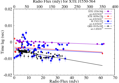
Figure 4: Correlation between radio flux and time lag is plotted for four objects. We opted for near simultaneous approach for the radio and time lag data. Each object was fitted with different slopes as properties of each objects may be vary. The gross slope was also found to be negative.

The correlation between radio flux and time is plotted in Fig. 4. We use the least square fitting method to obtain the slope and intercept. We separately fitted each curves corresponding to a particular source. All of the fitted curves show negative slopes which implicates the increase of soft lag with the increase in radio flux. Best fitted curve was obtained for XTE J1550-564 with the least amount slope. The reason behind it might be relatively lesser magnitude of soft lag which was detected during its 1998 outburst. Steepest slope was observed for GRS 1915+105. The reported lags (Muno et al. (2001), Dutta, Pal & Chakrabarti (2018)) for this candidate are much larger compared to others.

4.1 Test of Significance

We consider the null hypothesis

$$H_{0}=\mathrm{radio~{}jets~{}are~{}not~{}concurrent~{}with~{}soft~{}lags}$$

and the alternative hypothesis

$$H_{a}=\mathrm{radio~{}jets~{}are~{}concurrent~{}with~{}soft~{}lags}.$$

Our claim would strengthen if the null hypothesis is rejected. Level of confidence ($C$) is set to be $0.95$ or $95\%$. Accordingly, the test of significance $\alpha=1.0-C=0.05$. To establish the null hypothesis, we want to calculate the probability (p-value) of finding hard lags when radio flux $f_{\nu}\geq\bar{f_{\nu}^{h}}$ mJy which is essentially an “one sided right tail test”. So,

$$|Z|=\bigg{|}\frac{\bar{f_{\nu}^{h}}-\bar{f_{\nu}}}{(\sigma/\sqrt{N})}\bigg{|},$$

where $\bar{f_{\nu}^{h}}$ is the average of radio flux on the days where hard lags are seen, $\bar{f_{\nu}}$ is the global average of radio flux of a given candidate, $\sigma$ is the standard deviation and $N$ is the sample size. Thus, the probability of getting hard lags for $f_{\nu}\geq\bar{f_{\nu}^{h}}$ can be obtained from the standard chart using

$$P(Z:f_{\nu}\geq\bar{f_{\nu}^{h}})=1-P(Z:f_{\nu}\leq\bar{f_{\nu}^{h}}).$$

Table 2: Correlation Analysis.

Candidate Name	Pearson coefficient	Z score	$P(Z:f_{\nu}\geq\bar{f_{\nu}^{h}})$
XTE J1550-564	-0.754	2.26	0.012
XTE J1859+226	-0.673	2.14	0.016
H 1743-322	-0.495	6.05	$\leq 0.0003$
GRS 1915+105	-0.644	6.71	$\leq 0.0003$

We provide a chart with $Z$ scores and corresponding $P(Z)$ value for each candidates.

From the chart it is evident that $P(Z)\ll\alpha$. So, we can reject the null hypothesis.

5 Time Lag simulation

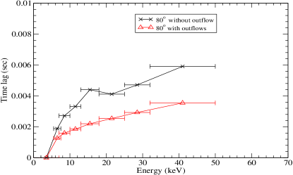
Figure 5: Simulated energy dependent time lags with and without the effect of outflows are presented for high inclination sources. The reference or soft band is 2.0 to 5.0 keV for simulated lag calculations. In presence of outflows, time lag magnitude decreases. Currently, simulation boundary extends up to 100 $r_{g}$ which is also the outer boundary of Keplerian disk. Outer boundary of Compton cloud is $~{}45~{}r_{g}$.

To mimic the features of an outburst, energy dependent time lags were simulated (CCG17b) considering relativistic thick disks as Compton cloud with decreasing outer boundary. The Keplerian disk acts as a soft photon source whose exterior was located at $100~{}r_{g}$. The outflow part was neglected (CCG17b) at first to simulate the lag spectra using anisotropic electron energy distribution in the Compton cloud. However, hydrodynamic simulation of sub-Keplerian flow allowed Chatterjee et al. (2018) to show time dependent images of disk-jet in presence of self-consistently produced outflows from Compton cloud. For similar outer boundary of the Compton cloud, the lag magnitude is found to be reduced (Fig. 5) for high inclination angle sources where outflows are considered.

6 Discussions: Possible Role of Outflows

One can infer a possible correlation between the soft lag and radio flux profiles from Fig. 2. To understand this behavior, we use two component advection flow solution which is based on transonic flow solutions around black holes (see CT95 for details). The model contains a high viscosity Keplerian disc on the equatorial plane which is surrounded by a low angular momentum advective component which produces a centrifugal barrier close to the black hole horizon. Numerical simulations of this advective component shows presence of strong winds Molteni et al. (1994) from the Compton cloud or CENtrifugal pressure supported BOundary Layer also known as CENBOL. Extending this to full general relativistic flow, recently Kim et al. (2019) showed that most of the outflow has sub-escape velocity and returns back to the equatorial region while only a fraction can achieve escape velocity and leave the system along the axis from Compton cloud. We conjecture that this return flow down-scatters hard photons and creates soft photons with large time lag. In principle, this should affect the time lag spectra of black holes. Since return flows are always associated with the jet activity, we find soft-lags to be higher when activity of the jets is also high. Figure 6 presents the cartoon diagram of the system. The effects mentioned above are only discernible for high inclination angle systems as gravitational bending enhances the number of hard photons (see CCG17a) which will eventually downscatter with the Returing OutFlows (ROF) along the line of sight of the observer.

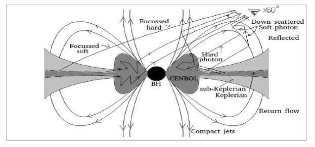
Figure 6: A cartoon diagram of the formation of jets and return flows from an advective disk is presented. Counting from the left side, six types of emergent photons are considered here. The first three photons are coming from the other side of the accretion disk and have suffered gravitational bending. Among them, the first one contributes in soft X-ray as it is not intercepted by the Compton cloud while the other two are inverse Comptonized. The fourth one is reflected and downscattered photon in the “ROF” region while the rest of the two types are hard photons which are downscatted in “ROF” and compact jet regions respectively.

Also, there may be other physical processes like lense-thirring precision (Ingram et al., 2009), disk reflection (Kara et al., 2013) which are proposed to be the contributor of the soft lags. Recently, (Schulze et al., 2017) a correlation between radio luminosity and measured spin of the Quasars suggested that the highly spinning black holes are more prone to be radio loud. This directly connects if soft lags were generated due to the spin of the central objects and their radio intensities. However, within our current studies, XTE J1550-564 showed most promising correlation between soft lags and radio intensities and the reported (Steiner et al., 2011) spin for that candidate is $0.49\pm 0.24$ indicating it to be an intermediate spin black hole. Using the Lamp-Post model proposed by Martocchia & Matt (1996) and Miniutti & Fabian (2004), the effect of outflows on lag behavior can also be understood. Outflow maximizes during the intermediate state where X-ray flux higher than the low state. During outflows (assuming the magnetic field of the lamp post corona drives out matter isotropically), number of photons reflected by the disk increases which could also enhance the soft lag magnitude (Kara et al. (2013), see §4). This could also explain the possible correlation between outflows and soft lags. Recently, Reig et al. (2018) showed correlations between photon index and lag magnitude. Their simulation (Reig & Kylafis (2019)) shows a correlation of the base of the jet and lag magnitude which can be interpreted as the change in spectral state. It would be interesting investigate such correlation changing the energy ($\varepsilon$), angular momentum ($\lambda$) and accretion rate ($\dot{m}$) (see for details Chakrabarti (1990)) in the hydrodynamic simulations of sub-Keplerian flow. But, the work is beyond the scope of this paper and will be reported elsewhere.

7 Conclusions

X-ray lags are important to understand the evolution of the geometry of an accretion disk and dominant physical mechanism. We showed here that soft lags are correlated with the radio intensity for some low mass X-ray binaries. We believe that this is a generic property of such systems since whether jets are produced ahead of outbursts (as in H1743-322) or during the outbursts, return flows will always downscatter hard photons as observed by high inclination systems. We conclude that:

1. 1. Soft-lags are concurrent with the radio flares.

2. 2. Outflows evolve with the evolution of disk. Along with Comptonization, reflection and effect of curved geometry (see DC16 and CCG17b), return outflows play a crucial role in the evolution of lag profiles.

3. 3. Our result demonstrates a model independent physical phenomenon which connect disk properties with jet activities.

Radio and X-ray time lag studies of a few GBHs at high inclination angle revealed new features in disk-jet paradigm. Recent works of Muno et al. (2001), Gandhi et al. (2008), Altamirano & Méndez (2015), Veledina et al. (2017), Malzac et al. (2018) and Tetarenko et al. (2019) have shown promising results on jet involvement with previously predicted disk activities. So, to understand more about the lag features and their origin, one must emphasize on the simultaneous broadband observations of black hole binaries.

8 Acknowledgements

AC acknowledges Post-doctoral fellowship of S. N. Bose National Centre for Basic Sciences and Indian Centre for Space Physics where a part of this work was carried out. BGD acknowledges IUCAA associateship. Authors thank Tomaso Belloni for providing the timing analysis software GHATS and anonymous Reviewer for suggestions and comments which enhanced the quality of the manuscript.

References

- Altamirano & Méndez (2015) Altamirano D. & Méndez M., 2015, MNRAS, 449, 4027
- Bardeen & Petterson (1975) Bardeen, J. M., & Petterson, J. A. 1975, ApJ, 195, L65
- Blanford & Begelman (1999) Blandford, R. D., & Begelman, M. C. 1999, MNRAS, 303, L1
- Brocksopp et al. (2002) Brocksopp C., Fender R. P., McCollough M., et al. 2002, MNRAS, 331, 7656
- Cadolle Bel et al. (2007) Cadolle Bel M. et al., 2007, ApJ, 659, 549
- Campbell-Wilson et al. (1998) Campbell-Wilson D., McIntyre V., Hunstead R. W., & Green A. 1998, IAU Circ., 7010, 3