Keywords:

Schrödinger equation; harmonic oscillator; logarithmic barriers; local large$-N$ expansions;

PACS number:

.

PACS 03.65.Ge - Solutions of wave equations: bound states

Abstract

Large$-N$ expansions are usually applied in single-well setups. We claim that this technique may offer an equally efficient constructive tool for potentials with more than one deep minimum. In an illustrative multi-well model this approach enables us to explain the phenomenon of an abrupt relocalization of ground state caused by a minor change of the couplings.

1 Introduction

The exact solvability makes the harmonic-oscillator models of bound states suitable for various quick estimates and qualitative phenomenological predictions. An amended fit of observed spectra is then usually achieved using an ad hoc  perturbation of the potential. In the resulting (say, one-dimensional) Schrödinger equation

$$\left[-\frac{\hbar^{2}}{2m}\frac{d^{2}}{dx^{2}}+\omega^{2}x^{2}+\lambda\,V_{(pert)}(x)\right]\,\psi_{n}(x)=E_{n}\,\psi_{n}(x)\,,\ \ \ \ n=0,1,\ldots\,$$ (1)

the user-friendliness of the conventional Rayleigh-Schrödinger perturbation expansions [1] then explains the widespread preference of the smooth power-law forms $V_{(pert)}(x)\sim x^{n}$ of the anharmonicities with, typically, $n=4$ or $n=6$ [2]. Alas, in contrast to the wealth of the emerging mathematical challenges [3], the strictly phenomenological impact of the quartic and sextic perturbations is not too impressive. These corrections only modify the shape of the potential far from its minimum. As a consequence, the influence of the perturbation is hardly felt by the low-lying, i.e., by the experimentally most relevant, bound states.

In our recent letter [4] we turned attention, therefore, to the possible consequences of using certain less usual value of a very small negative  exponent $n=-\alpha\approx 0$ for which the perturbation term $1/|x|^{\alpha}=1-\alpha\,\ln|x|+{\cal O}(\alpha^{2})$ is dominated, near the origin, by an infinitely high but still tunnelable repulsive barrier. For the non-power-law, short-range perturbations sampled by the logarithmic-function choice of $V_{(pert)}(x)\sim\ln|x|$ we revealed and verified that the study of the spiked-oscillator models of such a type may find an unexpectedly efficient solution method in the so called large$-N$ perturbation expansions (cf., e.g., the compact review paper [5] in this respect).

As a byproduct of the latter study we noticed that the introduction of a “soft”, weakly repulsive logarithmic central core in the potential

$$V_{eff}(x)=\omega^{2}x^{2}-g^{2}\,\ln|x|$$ (2)

enhances the pragmatic, descriptive appeal of the model. In the strong-coupling dynamical regime with $g^{2}\gg\omega^{2}$, for example, the system starts exhibiting certain features (like a pairwise degeneracy tendency of the low-lying even and odd states) which are usually attributed to the double-well models with a more strongly suppressed tunneling through the barrier.

Due to the left-right symmetry of our illustrative double-well soft-core model (2) (cf. also its square-well predecessor in [6]), multiple qualitative features of the bound-state spectra were found predictable a priori, without any extensive ad hoc  numerical or perturbative calculations which only confirmed the expectations. In our paper we intend to follow and extend this direction of research, therefore. We will consider certain more complicated shapes of the potentials with more than one logarithmic repulsive spike.

2 Large$-N$ method in nuce

The most elementary toy-model two-particle interactions $V(x)$ used in atomic, molecular and nuclear physics are very often composed of an asymptotically attractive harmonic-oscillator potential $V_{(attractive)}(x)=\omega^{2}x^{2}$ and of its short-range repulsive component. Typically, $V_{(repulsive)}(x)=g^{2}/x^{2}$ is used, at any number of particles $A$, in the popular $A-$body Calogero model [7]. This model is exactly solvable and, hence, suitable for our introductory illustrative and methodical purposes.

2.1 Calogero model in the strong-repulsion dynamical regime

In units such that $\hbar=2m=1$ the exactly solvable one-dimensional Schrödinger equation

$$\left[-\frac{d^{2}}{dx^{2}}+\frac{g^{2}}{x^{2}}+\omega^{2}x^{2}\right]\,\psi_{n}(x)=E_{n}\,\psi_{n}(x)\,,\ \ \ \ n=0,1,\ldots\,$$ (3)

with an impenetrable central barrier can be interpreted not only as the $A=2$ special case of the one-dimensional $A-$particle Calogero model (in which the attractive harmonic-oscillator two-body force is complemented by strong repulsion at short distances [7]) but also as a conventional radial component of a $D-$dimensional harmonic oscillator [2]. In both of these contexts, unfortunately, the barrier is impenetrable, not admitting a tunneling. As a consequence, not only the most common radial Schrödinger equation but also the more sophisticated Calogero’s equation must be perceived as living on a half-line or, in the Calogero’s case, as describing two independent systems defined in two separate “Weyl chambers” with $x\in(-\infty,0)$ and $x\in(0,\infty)$, respectively.

Any spontaneous transfer of the state of the system to the other chamber is, in the model, excluded. One must conclude that from the point of view of phenomenology the main weak point of the latter centrifugal-type repulsion is that it is impenetrable. Even in the most elementary two-body Calogero model the apparently double-well dynamics must be interpreted, in physics, as a pair of two independent single-well problems. At the same time, the model with the special choice of $g^{2}\gg\omega^{2}$ may serve as an illustrative example of the above-mentioned large$-N$ expansion techniques.

2.2 Oscillations near the deep local minima

The very essence of the efficient perturbative strong-coupling large$-N$ expansion technique lies in the approximation of the interaction. Near the deep minimum of $V_{eff}(x)$ at $x=R=R(N)$ the interaction is approximated by its truncated  Taylor series,

$$V_{eff}(x)\approx c_{0}+c_{1}(x-R)+c_{2}(x-R)^{2}+c_{3}(x-R)^{3}+\ldots+c_{M}(x-R)^{M}\,,\ \ \ \ \ c_{1}=0\,.$$ (4)

One of the most persuasive illustrations of the amazing practical numerical efficiency of such an approach is provided by the radial harmonic-oscillator Schrödinger equation

$$\left(-\frac{d^{2}}{dx^{2}}+x^{2}+\frac{N(N+1)}{x^{2}}\right)\ \psi_{m}(x)=E_{m}\ \psi_{m}(x)\,,\ \ \ \ \ N\gg 1\,,\ \ \ \ m=0,1,\ldots\,$$ (5)

in which the minimum of the complete effective interaction $V_{eff}(x)=x^{2}+{N(N+1)}/{x^{2}}$ lies at $x=R(N)=[N\,(N+1)]^{1/4}\gg 1$. In the Taylor series (4) we easily evaluate $c_{0}=V_{eff}(R)\gg 1$, $c_{2}={\cal O}(1)$ and $c_{2+j}={\cal O}(1/R^{j})$, $j=1,2,\ldots$. Thus, via an ad hoc  shift of coordinate $x\to x-R$ in Eq. (1) we found the constant $\omega^{2}=c_{2}$ as well as the desired small parameter $\lambda=1/R(N)$.

Needless to add that even the first nontrivial truncations of expansion (4) yield already a fairly reliable perturbative low-lying spectrum via Eq. (1) (cf. [4]). The problems only arise when we imagine that the approximate wave functions lie, by construction, on the whole real line, $x\in(-\infty,\infty)$. This appears to be a decisive conceptual shortcoming of the application of the method to Eq. (5) because as long as the centrifugal barrier does not admit tunneling, the exact bound states $\psi_{m}(x)$ do only live on the half-axis, $x\in(0,\infty)$. For this reason, the large$-N$ approximants cannot converge [5, 8].

In practice, fortunately, the $M\to\infty$ divergence of the Taylor-series potentials (4) is only rather weakly felt by the low lying approximate energies themselves. In the related literature, numerous tests of their $M-$th order large$-N$ alias  small$-\lambda$ representation

$$E_{m}(\lambda)=E_{m}(0)+\lambda\,E_{m}^{(1)}+\lambda^{2}\,E_{m}^{(2)}+\ldots+\lambda^{M}\,E_{m}^{(M)}+{\cal O}(\lambda^{M+1})\,$$ (6)

were performed for many phenomenological single-well-dominated interactions $V_{eff}(x)$ [9]. Most of these tests confirmed that the loss of the precision (reflecting the $M\to\infty$ divergence) only starts to influence the reliability of the results at certain optimal perturbation-expansion orders $M=M_{optimal}(\lambda)<\infty$.

2.3 Penetrable barriers

2.3.1 Complexified centrifugal term

One of the first amendments of the chamber-separation arrangement has been found in the framework of ${\cal PT}-$symmetric quantum mechanics. In this formulation of quantum theory [10, 11, 12] the tunneling between Weyl chambers implying a “relocalization” of the system on the real line of $x$ has been rendered possible via an ad hoc  regularization of the centrifugal-like barrier by its complexification,

$$\frac{g^{2}}{x^{2}}\ \to\ \frac{g^{2}}{(x-{\rm i}\varepsilon)^{2}}=\frac{x^{2}-\varepsilon^{2}}{(x^{2}+\varepsilon^{2})^{2}}+{\rm i}\frac{2\,\varepsilon\,x\ }{(x^{2}+\varepsilon^{2})^{2}}\ .$$ (7)

At $A=2$ [13] and at $A=3$ [14] it has been shown that in spite of the manifest non-Hermiticity of the complexified Calogero Hamiltonians the spectrum of the energies remains real and given in closed form. Reflecting, nicely, the nontrivial effects and consequences of the tunneling.

The latter two proposals using non-Hermitian interactions remained incomplete because the construction of the related physical Hilbert space (i.e., of a nontrivial inner-product metric $\Theta$ yielding the correct probabilistic interpretation of wave functions) proved prohibitively difficult [15]. In the light of some recent rigorous mathematical analyses, moreover, open questions still concern even the very existence of any  inner-product metric in such a local-interaction class of non-self-adjoint Hamiltonians [16, 17].

2.3.2 Central logarithmic spike

An easier way towards an amended model with tunneling has subsequently been proposed in [18]. In the framework of an entirely conventional quantum mechanics we merely replaced the complex spike (7) by the most elementary Hermitian point-interaction delta-function barrier which admits tunneling as well. We concluded that the property of the impenetrability of the centrifugal barrier in Eq. (5) is, for the reliability of the method, inessential.

The analytic, smooth logarithmic barrier of Refs. [4, 6] emerges as one of the other eligible candidates for a partially penetrable barrier, therefore. In loc. cit. we replaced the exactly solvable radial bound-state problem (3) by the harmonic oscillator Schrödinger equation perturbed by the logarithmic repulsive spike,

$$\frac{g^{2}}{x^{2}}\ \to\ g^{2}\,\ln\,\frac{1{\ }}{x^{2}}=-2\,g^{2}\,\ln\,|x|\,.$$ (8)

The new Schrödinger equation has been found solvable by the large$-N$ perturbation expansion technique which proved applicable at all of the sufficiently large couplings $g^{2}\gg\omega^{2}$. One of the encouraging technical merits of the replacement (8) of the power of $x$ by the more complicated logarithmic function has been found in the not quite expected user-friendliness of algebraic manipulations. This was a discovery which served also as an initial inspiration of our present paper.

3 Potentials with multiple logarithmic spikes

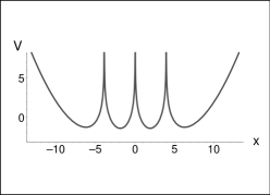
Figure 1: Illustrative four-well potential $V(x)=0.11\,x^{2}-\ln x^{2}-\ln(0.11\,x^{2}-1.7)^{2}$.

In the present paper we will pay attention to the following generalization of Eq. (8),

$$g^{2}\,\ln\frac{1}{x^{2}}\ \to\ g^{2}\,\ln\frac{1}{x^{2}}+\sum_{j=1}^{K}\,h^{2}_{j}\,\left(\ln\frac{1}{(x-s_{j})^{2}}+\ln\frac{1}{(x+s_{j})^{2}}\right)=-g^{2}\,\ln x^{2}-\sum_{j=1}^{K}\,h^{2}_{j}\,\ln(x^{2}-s_{j}^{2})^{2}\,.$$ (9)

Parameters $s_{j}>0$, $j=1,2,\ldots,K$ represent the (left-right symmetric) positions of the unbounded but still transparent logarithmic spikes converting the harmonic-oscillator well into a multi-well potential. An illustrative sample of its shape is displayed in Fig. 1. In a way inspired by such a quadruple-well example we decided to make the large$-N$ approach “localized”, restricted to any separate (and, presumably, still sufficiently pronounced and deep) minimum of the potential. We imagined that such an approach could open the way, e.g., towards a better understanding of the role of the small changes of the parameters which might influence, in a not entirely trivial manner, not only the positions of the separate minima of $V(x)$ but also the widths of the wells near these minima.

In the low-lying part of the spectrum such a simplification of the problem may be expected to enhance our understanding of what happens with the role of the minima of the potential which represent the eligible stable equilibria in classical systems. Naturally, this possibility follows from the absence of the tunneling so that the related picture of dynamics cannot be easily transferred to the quantum models with tunneling.

3.1 Large$-N$ pattern at $K=0$

After the “softening” (8) of the barrier the spatial symmetry of the $K=0$ effective potential with $g\neq 0$ (and, say, with $x\in(0,\infty)$ in Eq. (2)) still enables us to deduce that

$$V(x)=\omega^{2}x^{2}-g^{2}\ln x^{2}\,,\ \ \ \ \ \ V^{\prime}(x)=2\,\omega^{2}x-2g^{2}/x\,,\ \ \ \ \ \ V^{\prime\prime}(x)=2\,\omega^{2}+2g^{2}/x^{2}\,,\ \ldots\,.$$ (10)

This localizes the minimum of the potential at $x=x_{min}=R=g/\omega$ and defines the small parameter $\lambda=1/R$. With $e=2.718\ldots$ and $V^{\prime}(R)=0$ we have

$$V(R)=\omega^{2}R^{2}-2g^{2}\ln R=g^{2}\,\left(1-2\ln g+2\ln\omega\right)=g^{2}\,\ln(e\,\omega^{2}/g^{2})\,,\ \ \ \ \ \ V^{\prime\prime}(R)=4\,\omega^{2}\,,\ \ldots\,$$ (11)

in the truncated Taylor series (4). One also easily defines the depth and width of the leading-order harmonic-oscillator potential and arrives at the leading-order energies as prescribed by Eq. (6),

$$E_{n}=g^{2}\,\ln(e\,\omega^{2}/g^{2})+\sqrt{2}(2n+1)\,\omega+{\cal O}(1/g)\,\,,\ \ \ n=0,1,\ldots\,.$$

For the sufficiently strong repulsion $g\gg 1$, these values are found to compare well with the brute-force numerical results (cf. [4]).

3.2 Large$-N$ pattern at $K>0$

For our present purposes, one of the key consequences of the mere marginal relevance of the convergence or divergence of the asymptotic “large$-N$ input” Taylor series (4) is that the reliability of the perturbation approximants as provided by expansions (6) is almost exclusively dependent on the local  depth and width of the potential well near its minimum. In other words, without any real loss of the reliability of the results one can admit the existence of arbitrarily many other, separate minima. Such a conclusion leads us to the very core of our present methodical message: Under the assumption of a sufficiently suppressive separation barriers between the neighboring minima of the potential, one can apply the large$-N$ approximation technology, separately, in every individual well. Subsequently, the key idea is that the global low-lying spectrum will be mostly localized in the deepest and widest individual well. A delocalization of the system may be expected to occur only in the “exceptional” scenarios in which there will be no clearly dominant single individual well (or, in the spatially symmetric arrangements, a symmetric non-central pair of dominant wells).

The presence of several  repulsive logarithmic spikes in the potentials will form a multiple-well potential with its minima separated by the logarithmic barriers which are unbounded but still penetrable. Due to the freedom in our choice of the number of the barriers as well as of their strengths and positions, a remarkable flexibility of the resulting shape of the potentials will be achieved. Fig. 1 offers a typical illustration in which the quadruple-well shape of the potential is specific in having also the comparable depths of the separate minima. An analogous multi-well shape of our potentials may be also obtained at $K=2$ (cf. Fig. 2), etc.

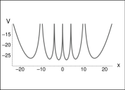
Figure 2: The shape of $V(x)=\omega^{2}\,x^{2}-g^{2}\,\log x^{2}-\lambda^{2}\,\log(\omega^{2}\,x^{2}-h^{2})^{2}-\mu^{2}\,\log(\omega^{2}\,x^{2}-f^{2})^{2}$ at $\omega^{2}=0.11,\,g^{2}=2\,,\lambda^{2}=2.3\,,h^{2}=1.7,\,\mu^{2}=5$ and $f^{2}=11.3$.

Remarkably enough, the latter descriptive merit of the model proves accompanied by an enhanced sensitivity of the depth of the separate minima to the comparatively small changes of the parameters. In the context of classical physics such a sensitivity is usually interpreted as opening a way towards a “catastrophe” [19]. In our present quantum-physics setting, such a sensitivity to the parameters must be interpreted more carefully of course [20].

3.3 An interplay between the widths and depths

In a way encouraged by the user-friendliness of the single-spike logarithmic $K=0$ anharmonic oscillator (cf. Eq. (10)) and of its large$-N$ description we believe that the study of the generalized, multi-well and left-right symmetric potential

$$V_{(K)}(x)=\omega^{2}x^{2}+g^{2}\,\ln\frac{1}{x^{2}}+\sum_{j=1}^{K}\,h^{2}_{j}\,\ln\frac{1}{(x^{2}-s_{j}^{2})^{2}}\,$$ (12)

(sampled in Fig. 2 at $K=2$) might be rewarding due to the variability of the integer $K=1,2,\ldots\,$. At the not too large values of $K$ the purpose of the approximate determination of the spectra may be seen in the prediction of the points of the relocalization instabilities. Indeed, the comparison of the large$-N$ spectra in the individual wells is probably one of the most reliable tools of the determination of the exceptional, “critical”, degeneracy-simulating sets of the parameters.

Any path defined in the space of parameters and passing through such a “relocalization” instability may be interpreted as an instant of transition of the system from its initial ground state localized, say, near the origin, to another ground state with probability density which is, near the origin, strongly suppressed. One can expect the experimental observability of such a phenomenon, especially in the low-lying-states setup.

In the context of theory we are, naturally, free to prefer working in the dynamical regime with strong repulsion in which the user-friendly large$-N$ solutions will lie sufficiently close to the exact ones. In our present paper we feel guided by the observation that a successful description of a given quantum system is often facilitated by the occurrence of a small parameter in the Hamiltonian, $H=H(\lambda)$. Typically, such a knowledge leads to a more or less routine expansion of the observable quantities in the powers of $\lambda$. In the multi-well potentials with a partially suppressed tunneling such an approach is simply to be implemented locally.

In the context of mathematics we intend to re-emphasize that the power series of perturbation theory need not be required convergent. The usefulness of the divergent alias  asymptotic series is best sampled by the large$-N$ expansion technique. The specific features of the technique enable one to use it for the description of qualitative aspects of the multiple-well dynamical scenarios.

4 Approximate bound states in individual wells

The generalized quantum bound-state problem

$$\left[-\frac{d^{2}}{dx^{2}}+V_{(K)}(x)\right]\,\psi_{n}(x)=E_{n}\,\psi_{n}(x)\,,\ \ \ \ n=0,1,\ldots\,,\ \ \ \ \psi_{n}(x)\in L^{2}(\mathbb{R})\,$$ (13)

is not too easily solvable even by the dedicated numerical methods. For this reason, its large$-N$ tractability would be welcome. In the light of our preceding comments, the approximate evaluation of the low-lying bound states may be expected helpful, especially when one of the wells dominates by its deptsh and width, and especially when the coupling constants $g^{2}$ and $h_{j}^{2}$ remain all  sufficiently large. Under such a restriction the various, topologically different multi-well versions Schrödinger bound-state problem (12) + (13) for low-lying states may still be given a user-friendly, perturbatively solvable form (1).

4.1 Truncated Taylor series

Once we decided to study Eq. (13) with potentials (12) in the strongly-spiked interaction regime, we feel entitled to split the wave functions into their separate (and, at the end, mutually matched)) components restricted just to one of the (presumably, deep) wells. This simplifies the general $2K-$ or $(2K+1)-$ barrier dynamical scenario and enables us to try to describe the bound states in an approximate, semi-qualitative manner.

The success of the strategy depends on several factors including the specification of the potential and the sensitivity of its shape to the variations of the parameters. The task is facilitated by several formal merits of our choice of the form of the potential. The key merit concerns the construction of the Taylor series for which one needs to know the derivatives of the potential. It is immediate to verify that the latter evaluation is straightforward, mainly due to the disappearance of the complicated logarithmic function after the differentiation. Thus, the elementary manipulations yield the necessary formulae

$$V^{\prime}_{(K)}(x)=2\,\omega^{2}x-\frac{2\,g^{2}}{x}-2\,\sum_{j=1}^{K}\,h^{2}_{j}\,\frac{2x}{x^{2}-s_{j}^{2}}\,,$$

$$V^{\prime\prime}_{(K)}(x)=2\,\omega^{2}+\frac{2\,g^{2}}{x^{2}}+4\,\sum_{j=1}^{K}\,h^{2}_{j}\,\frac{x^{2}+s_{j}^{2}}{(x^{2}-s_{j}^{2})^{2}}$$

and

$$V^{\prime\prime\prime}_{(K)}(x)=-\frac{4\,g^{2}}{x^{3}}-8x\,\sum_{j=1}^{K}\,h^{2}_{j}\,\frac{x^{2}+3\,s_{j}^{2}}{(x^{2}-s_{j}^{2})^{3}}$$

etc. In their light, the classification of the possible dynamical scenarios degenerates to the comparatively straightforward algebraic manipulations.

4.2 Example: Central well at $g=0$

At $g=0$ and at any $K$, one of the minima of $V_{(K)}(x)$ lies in the origin, $x=x_{0}=0$. At $K>0$ the locally minimal value of the potential is negative,

$$V_{(K)}(0)=-4\,\sum_{j=1}^{K}\,h^{2}_{j}\,\log{s_{j}}$$

(one should add that $V_{(0)}(0)=0$ at $K=0$). The local $M=2$ Taylor-series approximation of the potential degenerates to harmonic oscillator,

$$V_{(K)}(x)=V_{(K)}(0)+\frac{1}{2}\,V^{\prime\prime}_{(K)}(0)x^{2}+{\cal O}(x^{3})\approx V_{(K)}(0)+\Omega_{(K)}^{2}\,x^{2}\,.$$

Explicit formula is available for the real and positive

$$\Omega_{(K)}=\sqrt{\omega^{2}+\sum_{j=1}^{K}\,\frac{2\,h^{2}_{j}}{s_{j}^{2}}}\ .$$

Thus, whenever the central minimum is a global minimum, we may deduce the leading-order formula for the low-lying energies

$$E_{n}=V_{(K)}(0)+(2n+1)\Omega_{(K)}+{\rm corrections}\,,\ \ \ \ n=0,1,\ldots\,.$$ (14)

Otherwise, this formula just represents such a subset of the bound states for which the probability density is concentrated near the origin.

4.3 The role of parameters at $K=1$

4.3.1 Triple-well model with $g=0$

Besides the above-described central well the models with $g=0$ may exhibit also a $K-$plet of double-well non-central minima. In particular, in the first nontrivial case with $K=1$ the potential has the two off-central minima at $x=R_{(\pm)}$ where, by definition,

$$R_{(\pm)}=\pm\sqrt{s^{2}+\frac{2h^{2}}{\omega^{2}}}\,.$$

The two identical values of the other two local (and equal) extremes of the potential

$$V(R_{(\pm)})=\omega^{2}s^{2}+2h^{2}+h^{2}\log\frac{\omega^{4}}{4h^{4}}\,$$

lie at the other two non-central minima. Due to the positivity of the second Taylor-series coefficient

$$c_{2}=\Omega_{(\pm)}^{2}={\frac{1}{2}V^{\prime\prime}(R_{(\pm)})}={\omega^{2}+2\,h^{2}\,\frac{R^{2}+s^{2}}{(R^{2}-s^{2})^{2}}}={2\omega^{2}+\frac{s^{2}\omega^{4}}{h^{2}}}\,$$

we may evaluate the almost degenerate pair of the approximate double-well energies

$$E_{n}^{(\pm)}=\omega^{2}s^{2}+2h^{2}+h^{2}\log\frac{\omega^{4}}{4h^{4}}+(2n+1)\omega\,\sqrt{2+\frac{s^{2}\omega^{2}}{h^{2}}}+{\cal O}(1/h)\,,\ \ \ \ n=0,1,\ldots\,.$$ (15)

This formula complements the central harmonic-oscillator approximation of paragraph 4.2. In the generic case one of these parts of the spectrum is dominant (i.e., low-lying) while the other one remains highly excited.

At an exceptional instant of the relocalization catastrophe both of these candidates for the ground state (as well as, in principle, for the first few low lying excited states) remain comparable. In this case the leading-order large$-N$ approximation ceases to be applicable. The exact numerical solutions must be constructed instead.

4.3.2 Quadruple-well model with $g\gg\omega$

At $K=1$ the condition $V^{\prime}_{(K)}(R)=0$ for an extreme at $x=R=\sqrt{Z}\neq 0$ has the form

$$\omega^{2}Z-{g^{2}}-h^{2}\,\frac{2Z}{Z-s^{2}}=0\,.$$

This is a quadratic equation yielding the two positive roots

$$Z_{\pm}=\frac{1}{2}(a+c\pm\sqrt{2\,a\,c+b^{2}})\,,\ \ \ \ a=s^{2}+g^{2}/\omega^{2}\,,\ \ \ \ b=s^{2}-g^{2}/\omega^{2}\,,\ \ \ \ c=2\,h^{2}/\omega^{2}\,.$$

Their insertion leads immediately to a lengthy but explicit algebraic formula for the value of the coefficient $c_{2}=1/2\,V^{\prime\prime}_{(1)}(\sqrt{Z_{\pm}})$ entering the Taylor series (4) which defines the approximate harmonic-oscillator potential. Subsequently, one immediately obtains the low-lying energy spectrum for the states which are localized near the respective local minimum of the global potential function $V_{(1)}(x)$.

5 Conclusions

In the generic multi-well systems the descriptions of bound states can rarely be performed by non-numerical means. In our paper we verified that a slightly modified version of the large$-N$ approximation approach may simplify the constructions and offer an alternative, more straightforward mathematical tool.

In the context of quantum physics we paid particular attention to the fact that the control of the coupling constants in the potential immediately controls also the occurrence, properties and localization of the low-lying bound states. We emphasized that in the vicinity of a certain exceptional set of parameters, a comparatively small change of these parameters may lead to an abrupt “relocalization” jump in the particle probability density.

The presence of the repulsive barriers has been shown to play a decisive role in the possible interpretation of the states which are highly sensitive to the changes of the external conditions. Such states can be perceived as quantum analogues of the classical systems passing through an instability. Naturally, the analogy is incomplete, mainly because the Thom’s classification of the classical “catastrophes” did not find its sufficiently universal quantum-theoretical counterpart in mathematical literature yet [20].

5.1 Double-well models and quantum catastrophes

One of the most characteristic features of any  bound-state Schrödinger equation (13) with any  conventional symmetric double-well interaction potential $V(x)=V(-x)$ is that the first excited-state energy $E_{1}$ does not lie too far from its ground-state predecessor $E_{0}$. Intuitively, the phenomenon is explained by the existence of a central repulsive barrier which suppresses the central part of the wave function. The energy of the even ground-state wave function $\psi_{0}(x)$ without a nodal zero lies close to its first-excitation partner and odd wave function $\psi_{1}(x)$ possessing a single nodal zero in the origin.

In Ref. [4] we have shown that such a level-degeneracy tendency is observed, in the lowest part of the spectrum at least, even for the very weak (viz., logarithmic) central repulsive barriers such that $V(x)\sim\ln(1/x^{2})+{\cal O}(1)$ near the origin. At the same time, the effect may become quickly lost after the breakdown of the spatial symmetry of the potential. In general, one of the minima then becomes perceivably deeper and starts playing the dominant role in the localization of the low-lying wave functions. The closest classical analogue of such a phenomenon can be seen in the Thom’s catastrophes called “fold” or “cusp” [21].

5.2 More wells

In the context of the classical catastrophe theory [21] it is rather surprising to notice that in the literature, not too much attention is being paid to the more general quantum dynamical scenarios in which the number of the “tunable” minima of potential $V(x)$ is chosen greater than two. In our present paper we outlined a way towards the simulations of the less elementary quantum catastrophes. The tests of the idea were performed using a model with several application-oriented merits. One of them may be seen in the form of the individual barriers which remain singular (i.e., unbounded) but still much weaker than any power of $x$. Hence, the barriers admit a tunneling which is comparatively intensive even in the not too high energy levels. Still, the existence of the barriers leads to the localization of the wave functions near the deep minima of the potential. One only has to keep in mind that the lowest, ground state is often localized in the widest rather than in the deepest well or wells.

A subtler interplay between the separate individual wells only enters the game when none of the approximate ground-state energy-level candidates happens to dominate. This implies that the wave functions become “delocalized”, spread over several competing wells. In this critical dynamical regime our present method based on the identification of the dominant well (or rather of the dominant pair of wells) ceases to be applicable. This being said, even the use of approximants enables us to study the forms and alternative scenarios of the unfolding of the eligible quantum-catastrophic phenomena.

Acknowledgements

The project was supported by GAČR Grant Nr. 16-22945S.

References

- [1] A. Messiah, Quantum Mechanics I & II. North Holland, Amsterdam, 1961.
- [2] S. Flügge, Practical Quantum Mechanics I. Springer, Berlin, 1971.
- [3] T. Kato, Perturbation theory for linear operators. Springer, Berlin, 1966.
- [4] M. Znojil and I. Semorádová, Mod. Phys. Lett. A 33 (2018) 1850223.
- [5] N. E. J. Bjerrum-Bohr, J. Math. Phys. 41 (2000) 2515 - 2536.
- [6] M. Znojil, F. Růžička and K. G. Zloshchastiev, Symmetry 9 (2017) 165; M. Znojil and I. Semorádová, Mod. Phys. Lett. A 33 (2018) 1850009.
- [7] F. Calogero, J. Math. Phys. 10 (1969) 2191 and 2197, and J. Math. Phys. 12 (1971) 419; M. Znojil, J. Phys. A: Math. Gen. 36 (2003) 9929 - 9941.
- [8] V. I. Arnold, Catastrophe Theory. Springer-Verlag, Berlin, 1992.
- [9] U. Sukhatme and T. Imbo, Phys. Rev. D 28 (1983) 418; L. D. Mlodinow and M. P. Shatz, J. Math. Phys. 25 (1984) 943; B. Roy, R. Roychoudhury and P. Roy, J. Phys. A 21 (1988) 1579; O. Mustafa and M. Odeh, J. Phys. A: Math. Gen. 33 (2000) 5207; M. Znojil, F. Gemperle and O. Mustafa, J. Phys. A: Math. Gen. 35 (2002) 5781 - 5793; O. Mustafa and M. Znojil, J. Phys. A: Math. Gen. 35 (2002) 8929 - 8942; F. M. Fernández, J. Phys. A: Math. Gen. 35 (2002) 10663 - 10667; H. Bíla, Czech. J. Phys. 54 (2004) 1049 - 1054; I. V. Andrianov, V. V. Danishevskyy and J. Awrejcewicz, J. Sound Vibr. 283 (2005) 561 - 571; M. Znojil and U. Günther, J. Phys. A: Math. Theor. 40 (2007) 7375 - 7388; M. Znojil, Phys. Lett. A 374 (2010) 807812; A. F. Ferrari, M. Gomes, C. A. Stechhahn, Phys. Rev. D 82 (2010) 045009; M. Znojil, Int. J. Theor. Phys. 53 (2014) 2549 - 2557.
- [10] C. M. Bender, Rep. Prog. Phys. 70 (2007) 947.
- [11] A. Mostafazadeh, Int. J. Geom. Meth. Mod. Phys. 07 (2010) 1191.
- [12] D. Krejčiřík, V. Lotoreichik and M. Znojil, Proc. Roy. Soc. A: Math. Phys. Eng. Sci. 474 (2018) 20180264.
- [13] M. Znojil, Phys. Lett. A 259 (1999) 220 - 223.
- [14] M. Znojil and M. Tater, J. Phys. A: Math. Gen. 34 (2001) 1793-1803; M. Znojil, J. Phys. A: Math. Gen. 34 (2001) 9585 - 9592.
- [15] J. - H. Chen, June 2008, private communication.
- [16] M. Znojil, Phys. Rev. D 78 (2008) 025026; M. Znojil, J. Phys. A: Math. Theor. 41 (2008) 292002.
- [17] F. Bagarello, J.-P. Gazeau, F. H. Szafraniec and M. Znojil, editors, Non-Selfadjoint Operators in Quantum Physics: Mathematical Aspects. Wiley, Hoboken, 2015.
- [18] M. Znojil and M. Tater, Phys. Lett. A 284 (2001) 225 - 230.
- [19] R. Thom, Structural Stability and Morphogenesis: An Outline of a General Theory of Models. Addison-Wesley, Reading, 1989.
- [20] M. Znojil, J. Phys. A: Math. Theor. 45 (2012) 444036.
- [21] E. C. Zeeman, Catastrophe Theory - Selected Papers 1972 1977. Addison-Wesley, Reading, 1977.