On the interpretation of Feynman diagrams, or, did the LHC experiments observe $H\rightarrow\gamma\gamma$?

Abstract

According to the received view Feynman diagrams are a bookkeeping device in complex perturbative calculations. Thus, they do not provide a representation or model of the underlying physical process. This view is in apparent tension with scientific practice in high energy physics, which analyses its data in terms of “channels”. For example the Higgs discovery was based on the observation of the decay $H\rightarrow\gamma\gamma$ – a process which can be easily represented by the corresponding Feynman diagrams. I take issue with this tension and show that on closer analysis the story of the Higgs discovery should be told differently.

1 Introduction

Probably most physicists (and philosophers of physics) would agree that Feynman diagrams do not represent or model the underlying physical process in any closer meaning of these terms. Instead, these diagrams are a calculational tool or “bookkeeping device” for perturbative calculations in quantum field theory. Expressed pointedly, they visualize formulae and not physical processes. In this paper I will support this claim.

However, common and successful scientific practice in high energy physics appears to be in tension with this view. Take as a prominent example the recent discovery of the Higgs boson. Here, according to the usual narrative, the Higgs was detected via its dominant decays, e.g. in the $H\rightarrow ZZ\rightarrow 4\ell$ (here, $\ell$ denotes an electron or a muon) or $H\rightarrow\gamma\gamma$ channel. These channels are characterized by a set of Feynman diagrams and the account of the production and decay processes is usually just a verbal description of the corresponding diagrams. If there really were such a close connection between the experimental measurement and single Feynman diagrams the literal reading of them would be strongly supported.

Now, the goal of this paper is twofold. First I will show that this tension is only apparent, that is, the Higgs discovery (which will serve as our case study) does not presuppose a realistic interpretation of Feynman diagrams. In turn this leads to our second claim, namely that the common parlance is misleading and that the story of the Higgs discovery needs to be told differently. Expressed pointedly, the LHC experiments did not observe a process like $H\rightarrow\gamma\gamma$ since the very category (“observation”) is not applicable. In order to avoid any misunderstanding, I do not question the correctness of the results. It is just that they do not support the common narrative which singles out individual amplitudes of the scattering matrix while the mathematical framework presupposes that all relevant contributions (and this could include irreducible background as well) are taken into account. That is, the corresponding analyses of ATLAS and CMS provide clear evidence for standard model cross-sections involving Higgs terms with a corresponding mass $m_{H}\approx 125$ GeV. In this more carefully specified sense it is certainly true that the Higgs has been discovered at LHC.

In order to substantiate these claims I need to provide the basis for the debate. Sec. 3 is devoted to the interpretation of Feynman diagrams. Much of the debate in the literature deals with specific aspects, like the status of “virtual particles”. We will briefly survey the arguments from the literature, widen the scope and introduce new arguments to strengthen the claim that Feynman diagrams have no representational or modeling function proper. All this conflicts with their visual nature and intuitive appeal – two aspects which have contributed to the success of this diagrammatic method. In fact, the origin of this ongoing debate can be traced back to the introduction of the Feynman diagrams in 1948 and their subsequent formalization by Dyson. In order to highlight this relation I will briefly indicate the historical roots of the debate in Sec. 2.

While all this should be rather uncontroversial, I believe that the specific application to the scientific practice in high energy physics is missing in the literature on this subject. In Sec. 4 I will therefore investigate the Higgs discovery at LHC as a case study. As indicated above our goal is to demonstrate that contrary to first impressions a literal reading of Feynman diagrams is not supported by these results.

In closing this introductory section I should say a few words regarding terminology and methodology. The reader may have noted that I do not distinguish between the alleged “representational” and the “modeling” function of Feynman diagrams. These notions are closely related, since the success of a model may be based on its ability to represent certain features of the target system. That is, I apply the term “model” in a rather conventional sense. Following Meinhard Kuhlmann (2010, p. 126) I will call the interpretation of Feynman diagrams “realistic” or “literal” when it is assumed that the elements of the diagrams can be mapped onto something in the outer physical world. Fortunately, one is not committed to any specific form of mapping; the literature contains suggestions ranging from “isomorphic”, “partially isomorphic” or even less formal requirements (Frigg and Hartmann, 2012). I believe that this captures the usual usage within modeling sciences, i.e. here models are studied in order to generate claims and to learn something about the target system (Frigg and Nguyen, 2017, p. 51).

At the same time there are other approaches to the concept of model in which the representational role is not the only (or even primary) function. For example Michael Stöltzner (2017a, b) has argued that Feynman diagrams should be viewed as models in the more sophisticated sense of “models as mediators” as suggested by Mary Morgan and Margaret Morrison (Morgan and Morrison, 1999). Here, models are granted a more autonomous function. On this view Feynman diagrams may have more complex representational functions than the one indicated above. I believe that this is an important line of research, even more so if one assumes that a modeling function of Feynman diagrams in the conventional sense is excluded. Our objective is exactly to strengthen this premise.

Letitia Meynell (2008) argues that Feynman diagrams do have a representational function. However, this claim is not based on any property of these diagrams which had been overlooked before. Instead, she weakens the requirements for representation by separating “representation” from “denotation”. By this move the epistemic function of Feynman diagrams is left open (Meynell, 2008, p. 56). While this is an interesting approach I believe that such a weaker notion of “representation” is at odds with its common understanding in science. In any event the point at issue in this paper is exactly the epistemic function of Feynman diagrams.

Finally, all this is loosely related to the realism-debate. According to a popular myth “representations” are like a mirror image or a copy of the represented object, i.e. they are “realistic representations” (Frigg and Nguyen, 2017, p. 50). Roman Frigg and James Nguyen remark that there are non-realistic representations and that “representation is a much broader notion than mirroring” (Frigg and Nguyen, 2017, p. 50). I will sometimes talk about Feynman diagrams as understood “literally” or being taken to “depict” or to “visualize” the physical process. However, this wording is not intended to suggest the narrow notion of “representation as mirroring”. The question is not whether the representation is “realistic” but whether the system represented is “real”. Thus, this minimal form of realism is usually presupposed, namely the independent existence of the target system. In this sense part of the debate about the interpretation of Feynman diagrams has been framed e.g. as the question “Are virtual particles real?” (compare e.g. Weingard (1988)).

2 A brief history of Feynman diagrams

Feynman diagrams made their first public appearance in a presentation of Richard P. Feynman at a small gathering of elite physicists at Pocono (Pennsylvania) in the spring of 1948 (Kaiser, 2005, p. 43). However, the reception was cold, presumably since this introduction was based on merely intuitive arguments (among them the unfamilar idea of path integrals) rather than supported by a mathematical basis which at that time did not exist (Schweber, 1994, p. 443). But this new diagrammatic technique captured the interest of Freeman Dyson, then a PhD student under Hans Bethe at Cornell where Feynman was staff member. Dyson managed to provide the derivation of the corresponding rules from the mathematical basis of quantum electrodynamics (QED) and systematized the use of the diagrams significantly. He showed the equivalence of the three approaches by Julian Schwinger, Tomonaga Sin-itiro and Feynman. By combining the virtues of these approaches he could even generalize the proof of renormalizability of QED (Dyson, 1949).

However, this technique did not spread on its own, especially since the first textbook treatments were available only after 1955 (Kaiser, 2005, p. 27). Instead it needed what David Kaiser has called a “postdoc cascade”. Dyson moved to Princeton for his second year of his Commonwealth Fellowship and introduced a group of fellow postdocs at the Institute in the application of the method. These people took positions in academia scattered across (mainly) the US and developed schools which practiced the application of Feynman diagrams further.

At the same time Feynman diagrams demonstrated a high plasticity, i.e. its use could be adopted to the needs of the local research groups and went soon beyond the original scope (Kaiser, 2005, p. 173ff). Initially designed for perturbative calculations within weakly coupled theories like quantum electrodynamics the diagrams soon found application in nuclear physics and meson theory. Here, only first order contributions could be classified with the help of the diagrams and higher order calculations were not even useful.

The application in meson theory was championed by Robert Marshak and his group at Rochester. Marshak was certainly not part of the “postdoc cascade” but had attended the Pocono meeting. Subsequently, he and his group benefited from frequent visits by Feynman over the next two years (Kaiser, 2005, p. 221). Thus, their use of the diagrams was more intuitive and framed into a particle language rather than the “Dysonian” style. Kaiser remarks at this point, that due to the

“[…] failure of perturbative approaches for treating nuclear forces, Feynman diagrams’ pictorial forms and calculational roles became more and more differentiated.” (Kaiser, 2005, p. 207)

Now, the expression “pictorial forms” points already to the question whether Feynman diagrams could be used to picture the underlying process. On this question Feynman and Dyson disagreed from the very beginning. As noted above it was Dyson who derived the “Feynman rules” for the translation of diagrams into the corresponding mathematical expression from a quantum field theoretical starting point. Before that he could not make any sense of them, or as he put it:

“Nobody but Dick [Feynman] could use his theory, because he was always invoking his intuition to make up the rules of the game as he went along. Until the rules were codified and made mathematically precise, I could not call it a theory.” (cited from Kaiser (2005, p. 188))

To Dyson, Feynman diagrams were essentially a bookkeeping device. In his lecture “Advanced quantum mechanics”, delivered at Cornell during autumn 1951, he expressed this pointedly:

“We have introduced the Feynman graphs simply as a convenient pictorial way of visualizing the analysis of an operator into its normal constituents. The graphs are just diagrams drawn on the paper.”

But he continues immediately:

“But according to Feynman, “Space-time Approach to Quantum Electrodynamics”, (Phys. Rev. 76 (1949) 769), the graphs are more than this. He regards the graphs as a picture of an actual process which is occurring physically in space-time.” (Dyson, 1951, p. 99)

According to Dyson the diagrams sole purpose is to visualize the formulae. Thus, while the above mentioned “pictorial” role and the separation from the mathematical underpinning was foreign to Dyson, it was apparently closer to Feynman’s thinking. This marks the “Feynman-Dyson split” as David Kaiser has dubbed this

“[…] tension between Feynman’s and Dyson’s positions, with their varying emphases on ‘intuition’ versus derivation, physical pictures versus topological indicators.” (Kaiser, 2005, p. 263)

Kaiser shows how textbooks covering Feynman diagrams enhance this tension. While they typically announce a presentation in accordance with Dyson’s rigorous derivation, they postpone this part until Feynman diagrams were introduced already – apparently intending the diagrams to speak for themselves (compare Kaiser (2005, Chap. 7)). This tradition continues until today. The excellent text by Matthew Schwartz (2014) for example introduces Feynman diagrams already in Sec. 4 while the derivation of the corresponding rules is postponed to Sec. 7.

It is of course the visual nature of Feynman diagrams which makes them a popular teaching tool and which is part of the explanation for their great success. Kaiser argues that especially the resemblance with Minkowski diagrams and also bubble-chamber images allowed them to be

“[…] taught in ways that borrowed from more elementary skills that had already become second nature for most young physicists.” (Kaiser, 2005, p. 23)

That is, the split which divided Feynman and Dyson widened in the course of this teaching tradition further. The resulting ambiguous or almost schizophrenic situation is exemplified by the following quote from a popular textbook first published in the late 1960s:

“Because of the unphysical properties of Feynman diagrams, many writers do not give them any physical interpretation at all, but simply regard them as a mnemonic device for writing down any term in the perturbation expansion. However, the diagrams are so vividly ‘physical-looking’, that it seems a bit extreme to completely reject any sort of physical interpretation whatsoever. […] Therefore, we shall here adopt a compromise attitude, i.e., we will ‘talk about’ the diagrams as if they were physical, but remember that in reality they are only ‘apparently physical’ or ‘quasi-physical’ ”. (Mattuck, 1967, p. 88)

What Richard Mattuck describes as a “compromise attitude” should confuse the readers very much and it is unclear why the language should not reflect the actual status of the denoted objects more closely.

3 Interpretation of Feynman diagrams

As remarked above, textbook authors who introduce Feynman diagrams many pages before its mathematical basis is explained apparently assume that they can somehow “speak for themselves”. Now, what do they say? A verbal description of them easily falls into the habit of giving a space-time or even causal account of the sequence of “events” pictured. Ubiquitous is talk about “electrons and positrons meeting at a vertex”, “up quarks transforming into down quarks upon emitting a W boson” or “Higgs particles decaying into top and anti-top quarks”. At the same time many textbook authors provide also a word of caution, like “one must not take this interpretation too literally” (Mandl and Shaw, 2010, p. 67). However, what exactly “too literally” means is usually left open.

In this section I show why this word of caution is more than justified, that is, why properties of Feynman diagrams are at odds with any representational or modeling function with regard to the underlying physical process. Until recently the literature on the interpretation of Feynman diagrams has been rather sparse. General discussions can be found in Brown (1996), Elkins (2008) and Meynell (2008). Probably the most systematic treatment was given by Kuhlmann (2010). The specific aspect of virtual particles has captured the interest of more authors (Bunge, 1970; Redhead, 1988; Weingard, 1988; Fox, 2008; Arthur, 2012). I not only combine and strengthen some of these arguments but will also provide new ones. Especially by exploiting the notion of “topological equivalence” a strong case against any literal reading can be made. Before doing so I need to introduce some technical background and terminology.

3.1 Technical background

Most of what we know about elementary particles comes from scattering experiments, i.e. regards the probability for observing specific final states, given a specifically prepared initial state. For two particles in the initial and final state the situation is schematically depicted in Fig. 1. Here, the interaction is depicted as a circle which may be called the “bubble of ignorance”. The operator which relates incoming and outgoing states is the so-called scattering matrix, formally defined as (Lahiri and Pal, 2000, p. 81):

$$S={\cal{T}}\left[\exp\left(-i\int_{-\infty}^{+\infty}d^{4}x{\cal{H}}_{I}\right)\right].$$ (1)

Here, ${\cal{T}}$ is the time-ordering operator and ${\cal{H}}_{I}$ the part of the Hamiltonian which describes the interaction. The range of integration indicates, that the interaction lasts only a finite time and that long before or long after the interaction the states are essentially free. The transition amplitude between such asymptotically free states $|i\rangle$ and $|f\rangle$ is now given by

$$\langle f|S|i\rangle=S_{fi}.$$ (2)

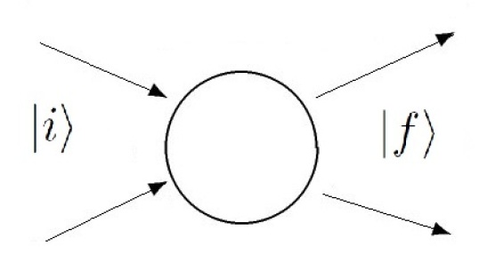
Figure 1: Schematic representation of a scattering process with two particles in the initial and final state. The circle in the center indicates the region of interaction.

To calculate this amplitude within QED or the Standard Model is very demanding. As a rule it can not be derived analytically and most predictions are obtained within perturbation theory, i.e. the solution is approximated by an expansion in powers of the coupling constant. Feynman diagrams are a tool to facilitate these calculations considerably. Each element of the calculation can be graphically displayed by a line or vertices between lines. Incoming and outgoing lines represent asymptotically free states and correspond to Dirac spinors (fermions) or polarization vectors (photons) in the calculation. The lines are directed to distinguish between particles and antiparticles. Internal lines correspond to a propagator or Green’s function $G(x-x^{\prime})$ in the calculation of the $S$ matrix element. They represent “virtual” particles, i.e. states which do not have to obey the relativistic energy-momentum relation:

$$E^{2}=p^{2}c^{2}+m^{2}c^{4}.$$ (3)

If they violate this relation they are said to be “off mass shell” or simply “off shell”.

The points where lines meet are called “vertices” and contribute a vertex factor, $g$, to the calculation. Further more the 4-momentum is conserved at each vertex. Expressed technically, all diagrams to a given order $n$ represent a term $S_{fi}^{(n)}$ in the expansion

$$S_{fi}\approx S_{fi}^{(0)}+gS_{fi}^{(1)}+\cdots+g^{N}S_{fi}^{(N)}.$$ (4)

Here, $N$ denotes the order of the approximation, i.e. the highest power of the vertex factor $g$ entering. This factor $g$ is related to the coupling constant by $g\propto\sqrt{\alpha}$. In QED $\alpha$ is the fine structure constant, i.e. $g$ is proportional to the electron charge. If the spin is taken into account the vertex factor includes an additional term. In addition symmetry factors and sign conventions form part of the Feynman rules if applied to more complex situations.

Now, the probability of the process is related to the square of the scattering matrix element:

$$P_{i\rightarrow f}\propto|S_{fi}|^{2}\approx\left|S_{fi}^{(0)}+gS_{fi}^{(1)}+\cdots+g^{N}S_{fi}^{(N)}\right|^{2}.$$ (5)

To calculate a (differential) cross-section, i.e. the observable quantity, one needs to include the information about the incoming flux and the available phase space of the corresponding process.

We now turn to the interpretation of Feynman diagrams. To begin with I will review some of the arguments from the lierature. The reader familiar with this debate may jump directly to Sec. 3.4 where a novel argument is introduced.

3.2 The “no-trajectory” argument

On the most naive realistic reading of Feynman diagrams they are taken to depict actual particle trajectories. Why this attempt is misguided is among the oldest arguments against such a literal reading. Famously the uncertainty relations exclude the existence of trajectories already in non-relativistic quantum mechanics. This was pointed out on the first public presentation of Feynman diagrams in 1948 at the Pocono meeting by Niels Bohr (Schweber, 1994, p. 444).

However, this is a rather weak argument since even Feynman in 1948 did not intend to picture particle trajectories and Niels Bohr acknowledged already at the Pocono meeting that this remark was based on a misconception (Mehra, 1994, p. 248). In fact, the existence of particle trajectories is no compulsory precondition for a realistic reading of Feynman diagrams (compare also Wüthrich (2012)). The following quote by one of the leading QFT experts and Nobel laureate Frank Wilczek is instructive:

“Feynman diagrams look to be pictures of processes that happen in space and time, and in a sense they are, but they should not be interpreted too literally. What they show are not rigid geometric trajectories, but more flexible, “topological” constructions, reflecting quantum uncertainty. In other words, you can be quite sloppy about the shape and configuration of the lines and squiggles, as long as you get the connections right.” (Wilczek, 2016)

Thus, by weakening the emphasis on the specific positions of the drawn elements compared to the overall “topological” structure an “almost literal” reading of the diagrams appears to be permitted.

This remark presumably alludes to the path integral approach to quantum theory. Famously, Feynman developed an alternative framework to quantum mechanics in which the probability amplitudes can be expressed as a sum (or rather functional integral) over all possible classical trajectories $x(t)$ weighted by the exponential of $i$ times the action ($e^{iS(x)/\hbar}$). This approach avoids the formalism of operators on Hilbert spaces. One may wonder how e.g. the uncertainty principle translates into this framework, given that it is usually associated with the non-commutativity of the corresponding operators. In the path integral approach the uncertainty relations reflect quantum fluctuations of the classical variables $x(t)$ and $p(t)$ (Kleinert, 2015, p. 927). Presumably this is the root of Wilczek speaking about “quantum uncertainty” in terms of “non-rigid trajectories”.

The path integral formalism can be generalized to cover (quantum) field theory. Again, the fields $\Phi(x)$ remain classical $c$-number fields and the quantum properties arise from the infinitely many integrals over $\Phi(x)$, one at each space time point $x$ (Kleinert, 2015, p. 934). While I will comment on the path integral approach to field quantization in some of the following sections, I should make the following general remark: The quantization via the path integral formalism has important applications (not only) in particle physics and may also provide additional insights into the underlying physics process. But since it yields the same Feynman rules of perturbation theory it provides no difference for the interpretation of Feynman diagrams as discussed below.

The above Wilczek quote mentions the “topological” aspects of Feynman diagrams and in Sec. 3.4 I will come back to this issue. There I will argue that the underlying “topological equivalence” provides a powerful argument against a realistic reading of Feynman diagrams.

3.3 The argument from superposition

The innocent looking square in Eq. 5 (or actually the square of the modulus of this complex number) is key to clear up some confusions about the interpretation of Feynman diagrams. To interpret a single term of this sum physically ignores the effects which underlie already the double-slit experiment in quantum mechanics. There, in a very similar way, the square of the sum of the contributions of the different slits yields the observable interference pattern and the question whether the electron “actually” went through slit 1 or 2 cannot be asked, let alone answered. In other words: the observed interference effects are related to all terms of the superposition. Conversely, a single term within a superposition does not refer to a physically realized process.

It might be objected, that there are cases in which a single diagram alone dominates the cross-section (see e.g. Valente (2011)). As noted by Kuhlmann (2010, p. 128) it is common talk to call higher order contributions ‘corrections’ to the ‘main process’ which is given by the leading order term. I believe that also here a literal reading of Feynman diagrams can not be supported. For one thing, a general interpretation of Feynman diagrams can not be based on specific processes. In fact, there are many cases, in which the leading order calculation involves more than one Feynman diagram already. In addition, to view the physical process as being build up of independent subprocesses (i.e. the ‘main process’ with additional ‘corrections’) produces false probabilities. On this view the observed probability should be given by the sum of the probabilities for each subprocess. Instead, each alleged “subprocess” contributes a term which has to be squared after summing to yield a probability.

In order to illustrate this point further, consider a cross-section for which the leading order term alone can account for, say, 90% of the observed value. This certainly does not support the claim that in 90% of the cases this process actually proceeds with the exchange of a single virtual particle only, while only in the other 10% the higher order terms which involve loop corrections and the “exchange” of many particles occur. In fact the observed process is always described by the whole series.

How this argument from superposition compromises the usual Higgs discovery narrative will be discussed in Sec. 4.3.

In the literature the argument from superposition has been used to compromise the notion of “virtual particles”, i.e. states depicted by the internal lines of Feynman diagrams which do not have to obey the relativistic energy-momentum constraint Eq. 3 (Redhead, 1988; Weingard, 1988; Fox, 2008). However, if the internal lines are void of any real meaning, there is not much left for Feynman diagrams to represent, that is, these arguments translate naturally into points against a literal reading of Feynman diagrams per se. Conversely, on a literal reading of Feynman diagrams one is committed to grant some physical meaning to “virtual” states.

As noted by Robert Weingard (1988) one reason for taking virtual particle states seriously comes from the action of creation and annihilation operators on them. In fact, the same operators that change the particle number of external (“real”) particle states act also on the internal states. Many textbooks on QFT invoke the energy-time uncertainty to make the notion of virtual particles plausible and explicitly claim that this relation implies the violation of energy conservation for the period $\Delta t\approx\hbar/\Delta E$. This argument is disturbing for several reasons, as noted already by Mario Bunge (1970). For one thing I do not know of any sound argument for the statement that in quantum mechanics energy is not conserved. Successful applications of the energy-time uncertainty relation deal e.g. with the energy-spread of states (say, the natural line width) and their lifetime. Now, according to the Feynman rules the constraint of energy-momentum conservation is met at each vertex. Thus, it is just the other way around: The internal lines representing “off-shell” states is a consequence of exactly this energy-momentum conservation – rather than being implied by any violation of this principle.

According to Robert Weingard (1988) and Tobias Fox (2008) the generic superposition states render the number and type of these “virtual particles” indefinite. These authors therefore view virtual particles as a mere artifact of the specific solution technique, namely perturbation theory. This view is further supported by the fact that the recursive method to solve field equations with the help of Green’s functions can also be applied for classical field equations. Also here the expansion can be depicted by “Feynman diagrams” with external and internal lines – thus there is nothing particularly “quantum” about them. Further more, within other solution techniques like lattice gauge theory no “virtual particles” emerge. Likewise, one may argue that “virtual particles” do not emerge in the path integral formulation of QFT, since no creation or annihilation operators enter the calculation of the Green’s function (Weingard, 1988, p. 47ff).

If one follows these arguments virtual particles should be viewed as fictitious. However, within the sophisticated model-debate in the philosophy of physics it has been suggested that models may actually (and rightfully) contain “fictitious” elements. Alisa Bokulich (2009) has pointed to the useful distinction between “explanatory fiction” and “mere fiction” in this context. Richard Arthur (2012) applies this distinction to virtual particles and provides strong arguments for the claim that they are “mere fiction”, i.e. serve no explanatory function.

3.4 The argument from “topological equivalence”

This brings us to an argument which – according to our knowledge – has not been exploited in the debate so far. Suppose that somebody is not convinced by the above argument from superposition. For example Mario Bacelar Valente (2011) argues in favor of virtual particles being more than a “formal tool”. He considers cases which are dominated by single diagrams and tries to exploit the fact that the $S$ matrix expansion is only asymptotic, i.e. that an infinite superposition is not involved.

However, what kind of “story” could a single Feynman diagram convey? Here one needs to recall an important concept from the theory of this diagrammatic technique. Feynman diagrams which can be continuously deformed into each other while leaving the in- and out coming states unchanged are called “topologically equivalent” (Mandl and Shaw, 2010, p. 68). Topologically equivalent diagrams depict the same amplitude and only one representative of this equivalence class needs to be considered (presumably this concept details the remark about “topological structures” in the above Wilczek quote; see Sec. 3.2).

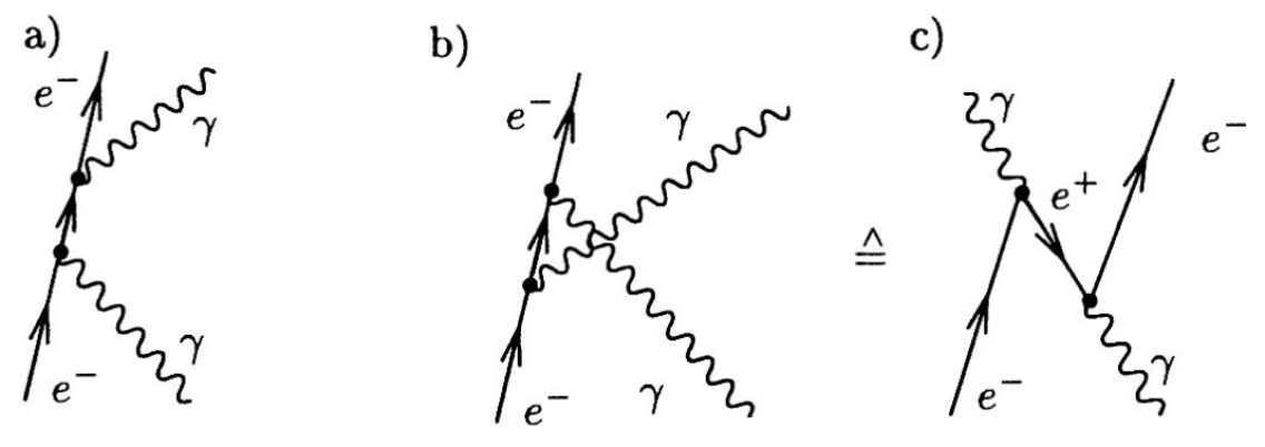
Figure 2: Feynman diagrams for Compton scattering in lowest order (time flow from bottom to top). In diagram a) a photon is first absorbed and subsequently emitted. The diagrams b) and c) differ only by time-ordering and are “topological equivalent”, i.e. it is sufficient to consider just one of them.

This fact can be easily turned into an argument against the literal interpretation of Feynman diagrams which tries to read a “sequence of events” into this graphical representation. Let us look at the example of Feynman diagrams depicted in Fig. 2 (time flow from bottom to top). They show the different contributions to the Compton scattering ($e^{-}\gamma\rightarrow e^{-}\gamma$) in lowest order perturbation theory. Fig. 2 a) seems to capture the intuitive sequence of “events”: first one photon is absorbed and subsequently one photon is emitted. However, already in lowest order another diagram needs to be considered as well. This is the one depicted in b) where photon emission and absorption reverse their time-order. This appears already counter-intuitive. However, an other – topological equivalent – diagram is shown in c). Here, the incoming photon splits into $e^{+}e^{-}$ while the incoming electron annihilates with the position to give rise to the final state photon. The electron of the pair creation is part of the final state. Thus, the stories which can be told to describe the diagrams b) and c) are quite different – they even involve different types of particles. But given their equivalence only one needs to be considered. They represent only different ways to draw the same diagram, consequently, the Feynman graphs do not support a specific “story” to be told about the underlying process.

In Sec. 4.4 this argument will be applied to question the usual narrative of the Higgs discovery.

3.5 Summary of the interpretation of Feynman diagrams

Summing up, there are major problems to sustain the view that Feynman diagrams represent any underlying physical process. This, in particular, affects the notion of “particle exchange” as mediating interactions. Friebe et al. suggest that this should be viewed as a metaphor only (Friebe et al., 2018, p. 242). For similar reasons James R. Brown (1996, p. 265) concludes that Feynman diagrams “do not picture any physical processes at all. Instead, they represent probabilities (actually, probability amplitudes)”. He compares them with Venn diagrams which also provide the visualization of an abstract relation (“being part of”), without claiming that the little circles resemble the corresponding system in any other respect. James Elkins comments in the same vein on the role of Feynman diagrams in the teaching of quantum field theory:

“Feynman diagrams are a useful calculational shorthand, but how helpful is a ‘learning tool’ that mispresents its object so deeply and leads people to misuse it so persistently?” (Elkins, 2008, p. 200)

He continues, that while Feynman diagrams no longer set out to resemble what they depict, the thinking about them is apparently influenced by a general attitude towards pictures:

“Yet, at the same time […] physicists, teachers, and students continue to think of them as if they could also have realistic properties – as if to say every picture must have some realism simply to be a picture.”(Elkins, 2008, p. 200)

In this respect Feynman diagrams share features with other visualizations in quantum theory. To use an other example given by Elkins (2008), the discrete spin values allowed by an electron are often depicted as vectors on a cone as if the electron would resemble a spinning top.

4 The Higgs discovery as a case study

Up to this point I have strengthened the received view which takes Feynman diagrams as a mere paper tool without representational function proper. However, at the same time this view is in apparent tension with successful scientific practice. Let us look at a recent example, namely the discovery of the Higgs boson at the Large Hadron Collider (LHC) announced in 2012, in order to connect our abstract findings about Feynman diagrams with the current research practice in high energy physics.

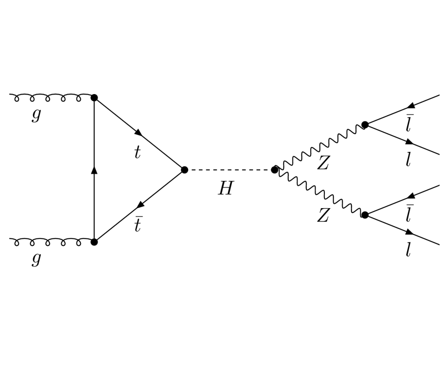
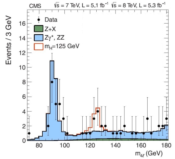
Figure 3: Left: Representative Feynman diagrams for the Higgs production via gluon-gluon fusion and decay into four charged leptons (time flow from left to right). Right: Distribution of the four-lepton invariant mass for the analysis of the $H\rightarrow ZZ\rightarrow 4\ell$ channel. The points represent the data, the filled histograms represent the background, and the open histogram shows the signal expectation for a Higgs boson of mass $m_{\mathrm{H}}=125$ GeV, added to the background expectation.

The dominant Higgs production mechanism at the LHC involves gluon-gluon fusion via an intermediate top-quark loop (see Fig. 3, left). The Higgs discovery was based on the analysis of specific decay channels; most importantly: $H\rightarrow\gamma\gamma$, $H\rightarrow ZZ\rightarrow 4\ell$ or $H\rightarrow WW\rightarrow 2\ell 2\nu$. Here, $\ell$ denotes a charged lepton. The corresponding publications (Aad et al., 2012; Chatrchyan et al., 2012) devote a subsection to each decay channel, i.e. report the results of the different analyses separately (clearly, they are combined subsequently). So, ATLAS and CMS have apparently “observed” the Higgs decay into two photons or four leptons separately. Contrary to what I said before, this seems to support the literal reading of single Feynman diagrams like the one displayed in Fig. 3 (left).

We should mention that the Higgs discovery publications by ATLAS and CMS do not contain Feynman diagrams but give reaction equations (as I did above). However, the announcement of the Higgs discovery by the CMS group in 2012 featured a very large number of Feynman diagrams. Also ATLAS used a few.

4.1 Higgs production

Let us examine this specific production channel ($gg\rightarrow H$) more closely. Already in leading order there are two Feynman diagrams which contribute to the top-loop mediated process $gg\rightarrow H$ (Bentvelsen, Laenen and Motylinsk, 2005); not to mention the contributions from other quark flavors. The LHC experiments use the next-to-next-to-leading order (NNLO) prediction from QCD and apply NLO electroweak corrections. In addition the effects of so-called “leading logs” have been considered to all orders (Aad et al., 2012, p. 2). Thus, to draw just a single diagram for the gluon-gluon fusion process $gg\rightarrow H$ is only a convenient shorthand for the whole partial series (Stöltzner, 2017a, p. 53). To the expert all this is certainly well known.

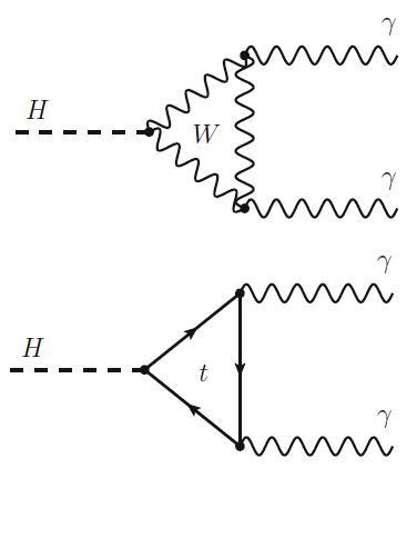
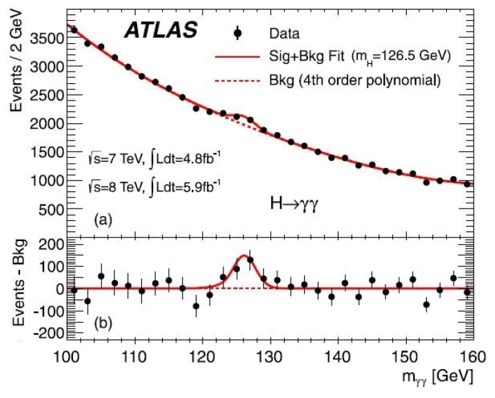
Figure 4: Left: Leading-order contributions to the decay of the Higgs boson into two photons. Right: Two-photon Invariant mass distribution as measured by ATLAS in the Higgs discovery paper.

4.2 Higgs decay

Let us move to the second part of the diagram, i.e. the Higgs decay channel $H\rightarrow ZZ\rightarrow 4\ell$ (in the LHC Higgs search the modes $\ell=e,\mu$ are considered). For one thing, if the final state contains identical leptons the corresponding interference effects need to be considered (Aad et al., 2012, p. 2). Again, this effect can not be read off the Feynman diagram as depicted in Fig. 3 (left). In the case of $H\rightarrow\gamma\gamma$ there is more than one contributions in leading order. As depicted in Fig. 4 (left) the decay may either proceed via an intermediate $W$-loop or fermion-loop. Due to its huge mass the top quark yields the dominant contribution. In cross section calculations the top loop enters with a minus sign, leading to a destructive interference term and lowering the overall decay rate into photons (Wolf, 2015, p. 93).

More importantly, one needs to ask how exactly this decay channel can be extracted from the data. In order to claim a discovery an experiment needs to show that the probability for the data being produced by a fluctuation of the known background is less that $5.8\cdot 10^{-7}$ (this corresponds, in the Gaussian limit, to the famous $5\sigma$ significance criterion). Given that the cross-section for the Higgs production is tiny compared to processes with similar signatures this background needs to be understood with extreme precision. In fact, the object of observation is not just the finally extracted signal, but the combination of many “processes”. In order to disentangle them one needs the knowledge of the relative fractions of all these cross-sections and has to normalize all contributions properly. Again, the evaluation of countless diagrams (not to mention the correction due to detector- and hadronisation effects) contributes to the final result.

A typical result of this analysis, taken form the CMS Higgs discovery paper, is shown in Fig. 3 (right). It shows the four-lepton invariant mass as reconstructed from the selected data (Chatrchyan et al., 2012). Most prominent is the $Z$ peak arround 91 GeV, which is due to resonant $Z$ production. In the range of 120 and 130 GeV an excess of events above the expected background can be seen. The open histogram corresponds to the Standard Model prediction with a Higgs mass of $m_{H}=125$ GeV and fits the data well. Only something like 15 events contribute to this Higgs signal. It is evident that in order to derive any result the background needs to be controlled with extreme precision.

Thus, it would be misleading to claim, that the analysis of the $H\rightarrow ZZ\rightarrow 4\ell$ channel just “measures” or “observes” the contribution from a single Feynman diagram; even if the signal as such is dominated by the contribution of only one or a few Feynman graphs indeed.

Agreed, a proper understanding of the background, calibration etc. is not specific to LHC physics. And indeed, an invariant mass distribution as the one in Fig. 3 (right) or the corresponding distribution for the decay channel $H\rightarrow\gamma\gamma$ (Fig. 4, right) seems to suggest that the underlying process is captured by “decay channel talk”. Apparently such a distribution is as close as one can get to actually “see” a Higgs boson via the corresponding decay. However, there is an additional twist to the argument. Suppose that the invariant mass distributions could be measured with highly improved accuracy. Would this distributions peak at the “actual” Higgs mass? The surprising (and to our mind not sufficiently emphasized) answer is no, as will be explained in the next subsection.

4.3 How to extract the Higgs mass – the superposition argument in the Higgs decay

If the invariant mass distribution in the $\gamma\gamma$ or $4\ell$ channel could be measured with highly improved accuracy the peak of the distribution would not correspond to the Higgs mass, since due to interference effects with the background the distribution gets shifted. This effect has been discussed for the channel $H\rightarrow ZZ$ by Kauer and Passarino (2012) and for the $H\rightarrow\gamma\gamma$ channel by Martin (2012). This last paper contains also the plot reproduced in Fig. 5 (left). Here, the right curve shows the Higgs contribution only, while the mass peak is shifted to lower values if the interference effects are taken into account. That is, in principle the Higgs mass can not be measured by directly fitting the mass-distribution in the corresponding plot, but only by comparing the full Standard Model prediction (with varying $m_{H}$ values) with the obtained distribution. Strictly speaking, the peak in the invariant mass distribution is not identical to the Higgs mass and the “process” $H\rightarrow\gamma\gamma$ can not be observed in isolation.

We agree that the shift in the mass distribution is rather small (estimated to $\approx 100$ MeV in the $\gamma\gamma$ channel (Martin, 2012, p. 4) and even smaller for the Higgs decaying into $ZZ$). The combined Higgs mass analysis of ATLAS and CMS neglects background interference although the result yields $m_{H}=125.09\pm 0.21(\mathrm{stat})\pm 0.11(\mathrm{sys})$ GeV (Aad et al., 2015). Actually an effect in the order of some 10 MeV should be a sizable contribution to the systematic uncertainty.

It goes without saying that all this is very well known in the community. The interference effect with the background are dealt with in detail in the yellow reports of the LHC Higgs Cross Section Working Group (see e.g. Heinemeyer et al. (2013, p. 35ff)). In the first volume of the Higgs working group report it is stated explicitly:

“[…] what the experiments observe in the final state is not always directly connected to a well defined theoretical quantity. We have to take into account the acceptance of the detector, the definition of signal, the interference signal-background, and all sorts of approximations built into the Monte Carlo codes. As an example at LEP, the line shape of the $Z$ for the final state with two electrons has to be extracted from the cross section of the process ($e^{+}e^{-}\rightarrow e^{+}e^{-}$), after having subtracted the contribution of the photon and the interference between the photon and the $Z$.” Dittmaier et al. (2011)[p. 2] (emphasis in the original)

In any event I take this numerically small effect to be of great conceptual importance. The interference between Higgs and background processes demonstrates that the whole talk about “Higgs decay channels” holds only approximately. The term “channel” suggests that all events can be grouped into disjoint classes, while actually interference takes place between signal and background contributions if the final states are the same. Given that the dominant contribution from resonant Higgs decays comes from the Higgs propagator the neglect of these interference effects are a justified approximation but do not challenge our previous claim about Feynman diagrams. The argument based on the superposition of amplitudes (see Sec. 3.3) remains valid since it does not presuppose that the corresponding effects are large – it just assumes that these effects are possible. Consequently, this valid numerical approximation does not support the intuitive picture of Higgs production and subsequent decay which follows from a literal reading of the Feynman diagrams. This narrative singles out specific (signal) amplitudes while the actual process is related to the squared sum of signal and background contributions. Thus, one is not talking about “ordinary” background which could be eliminated by applying more clever cuts or by subtraction. For these kinds of contributions the term “irreducible background” has been coined. The corresponding invariant mass plots show a Higgs signal, to be sure. Its mass can be deduced from it. But these plots do not display the Higgs mass.

It should be noted that ATLAS and CMS do not identify the mass peak with the Higgs boson explicitly. Instead, they call the corresponding region in their histograms “signal expectation” or “signal component” for a Higgs with $m_{H}=125$ GeV (Aad et al., 2012; Chatrchyan et al., 2012). However, as indicated above, also the separation into “signal” and “background” holds only approximately. For example the background in the $\gamma\gamma$ analysis was fitted by a polynomial and subtracted from the data to yield the lower inset of the plot in Fig. 4 (right).

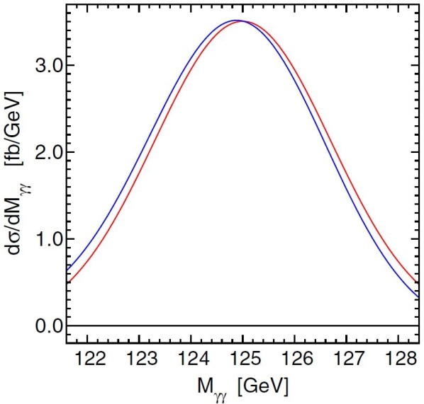
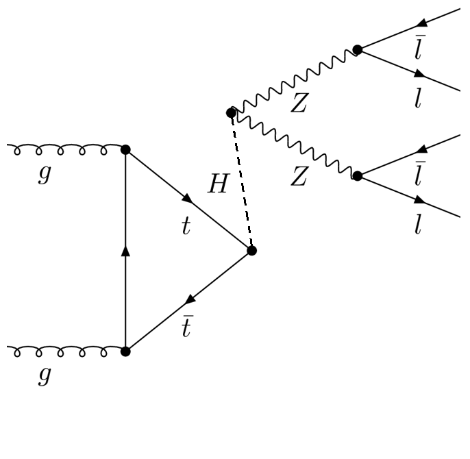
Figure 5: Left: Mass shift of the 2-photon invariant mass distribution due to interference effects with the background. The right curve shows the Higgs contribution only, while the mass peak is shifted to lower values if the interference effects are taken into account (Fig. taken from Martin (2012, Fig. 3)). Right: Topological equivalent Feynman diagram for one of the amplitudes which yield the dominant contribution in the Higgs discovery (time flow from left to right).

4.4 The argument from “topological equivalence” in the Higgs discovery

We have seen above how the argument from superposition compromises the literal reading of Feynman diagrams in the case of Higgs production and decay. The same is true for the argument from “topological equivalence” (see Sec. 3.4). Fig. 5 (right) shows a diagram which is equivalent to the one in Fig. 3 a). Here, the time-ordering of Higgs creation and annihilation is reversed. Under a literal understanding of Feynman diagrams the discovery would then be based on the Higgs production together with a pair of $Z$ bosons while the Higgs annihilates subsequently with a $t\bar{t}$-pair. Again, that is not the kind of story one wants to tell when dealing with a “Higgs production in the gluon-gluon channel” since it apparently deals with the top-loop induced Higgs annihilation instead.

Of course you may invent still other equivalent diagrams for the same amplitude. Fig. 6 gives an example where the $Z$-line was twisted away. Here the apparent “story” would be the production of lepton pairs together with a $Z$ which subsequently radiates off a Higgs boson. The $Z$ produces another pair of leptons in the final state while the Higgs annihilates again with top-pairs.

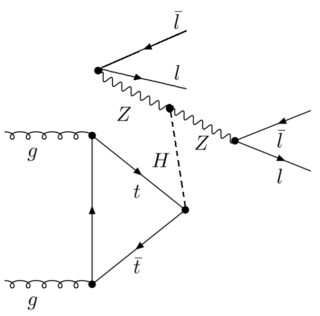
Figure 6: An other example for a topological equivalent Feynman diagram in the $H\rightarrow ZZ\rightarrow 4\ell$ channel.

Also here, the literal reading of Feynman diagrams can not be sustained and the inside of the “bubble of ignorance” remains unknown.

5 Summary and conclusion

We have argued that Feynman diagrams do not model or represent the underlying physical processes. While the often quoted “no-trajectory” argument may be circumvented, the argument from superposition questions the possibility to assign any meaning to a single Feynman diagram. However, even if individual diagrams could be interpreted physically, they would not provide a unique “sequence of events”. The notion of topological equivalence compromises a literal understanding of these “stick-figures” (Kaiser, 2000) further. Thus, Feynman diagrams picture formulae – not physical processes.

While all this just strengthens the received view I took issue with the apparent tension between this anti-realistic reading of Feynman diagrams and their use (and the common jargon) in high energy physics. For example in the Higgs discovery the common narrative appears to take Feynman diagrams as direct visualizations of a Higgs decaying into two photons or four leptons. The division into these distinct decay channels suggests disjoint classes in which the events can be grouped. Furthermore, a peak at $\approx 125$ GeV in the invariant mass spectrum apparently provides direct evidence for the corresponding Higgs decay channel to be observed.

However, an individual event can not be assigned to the “background” or “signal” category. If the final states are the same the observed process is the superposition of the contributions from the corresponding diagrams and interference occurs. This shows up for example in the invariant mass spectrum which does not peak (exactly) at the Higgs mass value. Likewise, the argument from topological equivalence can be applied to compromise an intuitive understanding of Higgs production and subsequent decay.

As expected, the tension between the anti-realistic reading of Feynman diagrams and the successful research practice is only apparent. Of course, the material presented in our Higgs case study is well known (not only) to the experts in the field. The reason why all these aspects do not figure prominently in the Higgs discovery lies in the fact that in resonant production the corresponding interference effects are numerically small and can not be experimentally resolved yet. It goes without saying that the Higgs analyses of ATLAS and CMS are admirable achievements and that the confirmation of the Higgs mechanism is an intellectual and technical masterpiece. The applied approximations are valid and I certainly do not question the discovery of the Higgs boson. However, the corresponding narrative promotes (unintentionally, I assume) a simplistic picture of particle physics in which a literal reading of Feynman diagrams is supported. In (non-relativistic) quantum mechanics it is usually a central claim that no causal or space-time picture of the process between preparation and measurement can be given. It is curious to note that on a literal reading of Feynman diagrams some authors apparently accept the risk to fall below this level.

Most importantly, the different amplitudes should not be confused with “physical processes”, given that the actual observation relates to the squared sum of all contributions. In this sense a contribution like $H\rightarrow\gamma\gamma$ can not be observed since this very category is not applicable. What has been successfully tested was the whole of the Standard Model including its account for electro-weak symmetry breaking.

As discussed in Sec. 2 David Kaiser has dubbed the tension between a more intuitive understanding versus the formal derivation of the diagrams the “Feynman-Dyson split”. He has noted that textbook presentations have enhanced this tension. Our case study reveals that the presentation of the current research practice in high energy physics likewise contributes to a widening of this split.

References

- Aad et al. (2012) Aad, G. et al. ATLAS Coll. (2012) Observation of a new particle in the search for the Standard Model Higgs boson with the ATLAS detector at the LHC. Phys. Lett. B 716(1) 1–29.
- Aad et al. (2015) Aad, G. ATLAS and CMS Coll. (2015) Combined Measurement of the Higgs Boson Mass in pp Collisions at and 8 TeV with the ATLAS and CMS Experiments. Phys. Rev. Lett. 114 191803 (33pp).
- Arthur (2012) Arthur, R. T. W. (2012) Virtual Processes and Quantum Tunnelling as Fictions. Sci & Edu 21:1461–1473.
- Bentvelsen, Laenen and Motylinsk (2005) Bentvelsen, S., Laenen, E. and Motylinski, P. (2005) Higgs production through gluon fusion at leading order. NIKEF 2005-007.
- Bokulich (2009) Bokulich, A. (2009) Explanatory Fictions. In: M Suárez (ed) Fictions in Science: Philosophical Essays on Modeling and Idealization New York: Routledge (pp. 91–109).
- Brown (1996) Brown, J. R. (1996) Illustration and Inference. In: Picturing Knowledge: Historical and Philosophical Problems Concerning the Use of Art in Science B. Baigrie (ed.). Toronto: University of Toronto Press pp 250–268.
- Bunge (1970) Bunge, M. (1970) Virtual processes and virtual particles: Real or fictitious? Int. J. Theo. Phys. 3(6) 507–508.
- Chatrchyan et al. (2012) Chatrchyan, S. et al. CMS Coll. (2012) Observation of a new boson at a mass of 125 GeV with the CMS experiment at the LHC. Phys. Lett. B 716(1) 30–61.
- Dittmaier et al. (2011) Dittmaier, S., Mariotti, C., Passarino, G. und Tanaka, R. (Hrg.) (2011) Handbook of LHC Higgs Cross Sections: 1. Inclusive Observables. Report of the LHC Higgs Cross Section Working Group, http://xxx.lanl.gov/abs/1101.0593.
- Dixin and Li (2013) Dixon, L. J. and Li, Y. (2013) Bounding the Higgs Boson Width through Interferometry. Phys. Rev. Lett. 111 111802 (5pp).
- Dyson (1949) Dyson, F. J. (1949) The Radiation Theory of Tomonaga, Schwinger, and Feynman. Phys. Rev. 75(3) 486–502.
- Dyson (1951) Dyson, F. J. (1951) Advanced quantum mechanics. The typed and annotated version of the original typoscript is available at quant-ph/0608140.
- Elkins (2008) Elkins, J. (2008) Six Stories from the End of Representation. Stanford: Stanford University Press.
- Feynman (1949) Feynman, R. P. (1949) Space-Time Approach to Quantum Electrodynamics. Phys. Rev. 76(6) 769–789
- Fox (2008) Fox, T. (2008) Haunted by the spectre of virtual particles: A philosophical reconsideration. J. Gen. Phil. Sci 39(1), 35–51
- Friebe et al. (2018) Friebe, C., Kuhlmann, M., Lyre, H., Näger, P., Passon, O. and Stöckler, M. (2015) The Philosophy of Quantum Physics. Berlin, Heidelberg: Springer.
- Frigg and Hartmann (2012) Frigg, R. and Hartmann, S. (2012) Models in Science. The Stanford Encyclopedia of Philosophy (Spring 2017 Edition), Edward N. Zalta (ed.).
- Frigg and Nguyen (2017) Frigg, R. and Nguyen, J. (2017) Models and Representation. In Lorenzo Magnani and Tommaso Bertolotti (eds.) Springer Handbook of Model-Based Science Dordrecht, Heidelberg, London and New York: Springer (pp. 49–102).
- Heinemeyer et al. (2013) Heinemeyer, S., Mariotti, C., Passarino, G. und Tanaka, R. (Hrg.) (2013) Handbook of LHC Higgs cross sections: 3. Higgs Properties. Report of the LHC Higgs Cross Section Working Group, http://xxx.lanl.gov/abs/1307.1347.
- Kaiser (2000) Kaiser, D. (2000) Stick-Figure Realism: Conventions, Reification, and the Persistence of Feynman Diagrams, 1948–1964. Representations 70 49–86.
- Kaiser (2005) Kaiser, D. 2005 Drawing Theories Apart. Chicago: The University of Chicago press.
- Kauer and Passarino (2012) Kauer, N. and Passarino, G. (2012) Inadequacy of zero-width approximation for a light Higgs boson signal. J. High Energ. Phys. 1208 116.
- Kleinert (2015) Kleinert, H. (2015) Particles and Quantum Fields. Singapore: World Scientific.
- Kuhlmann (2010) Kuhlmann, M. (2010) The Ultimate Constituents of the Material World. Frankfurt a. M.:Ontos.
- Lahiri and Pal (2000) Lahiri, A. and Pal, P. B. (2000) A first Book on Quantum Field Theory. Oxford, UK.: Alpha Science.
- Mandl and Shaw (2010) Mandl, F. and Shaw, G. (2010) Quantum Field Theory. (Second edition) Chichester: Wiley.
- Martin (2012) Martin, S. P. (2012) Shift in the LHC Higgs diphoton mass peak from interference with background. Phys. Rev. D 86 073016 (6pp).
- Mattuck (1967) Mattuck, J. (1967) A guide to Feynman diagrams in the many-body problem. (second edition) New York: Dover.
- Mehra (1994) Mehra, J. (1994) The Beat of a Different Drum Oxford: Clarendon.
- Meynell (2008) Meynell, L. (2008) Why Feynman Diagrams Represent. International Studies. Philosophy of Science 22(1) 39–59.
- Morgan and Morrison (1999) Morgan, M. and Morrison, M. (eds.) (1999) Models as Mediators: Perspectives on Natural and Social Science. Cambridge: Cambridge University Press.
- Peierls (1985) Peierls, R. (1985) Bird of Passage – Recollections of a Physicist. Princeton: Princeton University Press.
- Redhead (1988) Redhead, M. (1988) A philosopher looks at quantum field theory. In: H. R. Brown and R. Harré (Eds.) Philosophical foundations of quantum field theory Oxford: Clarendon Press.
- Schwartz (2014) Schwartz, M. D. (2014) Quantum Field Theory and the Standard Model. Cambridge: Cambridge University Press.
- Schweber (1994) Schweber, S. S. (1994) QED and the men who made it. Princeton: Princeton University Press.
- Stöltzner (2017a) Stöltzner, M. (2017a) Feynman Diagrams as Models. The Mathematical Intelligencer 39(2) 46–54.
- Stöltzner (2017b) Stöltzner, M. (2017b) Feynman Diagrams: Modeling between Physics and Mathematics. forthcoming.
- Valente (2011) Valente, M. B. (2011) Are Virtual Quanta Nothing but Formal Tools? International Studies in the Philosophy of Science 25(1): 39–53.
- Weingard (1988) Weingard, R. (1988) Virtual particles and the interpretation of quantum field theory. In: H. R. Brown and R. Harré (Eds.) Philosophical foundations of quantum field theory Oxford: Clarendon Press.
- Wilczek (2016) Wilczek, F. (2016) How Feynman Diagrams Almost Saved Space. Quanta Magazine.
- Wolf (2015) Wolf, R. (2015) The Higgs Boson Discovery at the Large Hadron Collider Springer Tracts in Modern Physics, Volume 264, Heidelberg: Springer.
- Wüthrich (2010) Wüthrich, A. (2010) The Genesis of Feynman Diagrams. Berlin, Heidelberg: Springer.
- Wüthrich (2012) Wüthrich, A. (2012) Interpreting Feynman Diagrams as Visual Models. Spontaneous Generations: A Journal for the History and Philosophy of Science 6(1): 172–181.