Interpretable BoW Networks for Adversarial Example Detection

Abstract

The standard approach to providing interpretability to deep convolutional neural networks (CNNs) consists of visualizing either their feature maps, or the image regions that contribute the most to the prediction. In this paper, we introduce an alternative strategy to interpret the results of a CNN. To this end, we leverage a Bag of visual Word representation within the network and associate a visual and semantic meaning to the corresponding codebook elements via the use of a generative adversarial network. The reason behind the prediction for a new sample can then be interpreted by looking at the visual representation of the most highly activated codeword. We then propose to exploit our interpretable BoW networks for adversarial example detection. To this end, we build upon the intuition that, while adversarial samples look very similar to real images, to produce incorrect predictions, they should activate codewords with a significantly different visual representation. We therefore cast the adversarial example detection problem as that of comparing the input image with the most highly activated visual codeword. As evidenced by our experiments, this allows us to outperform the state-of-the-art adversarial example detection methods on standard benchmarks, independently of the attack strategy.

1 Introduction

While the discriminative power of deep convolutional neural networks (CNNs) is nowadays virtually uncontested, one of the key research challenges that remain unaddressed is their interpretability; in many practical scenarios, one is not only interested in obtaining a prediction from the network, but also in understanding the reason behind this prediction. The main trends to tackle interpretability consist of post-training analysis to visualize either feature maps at different layers [36, 35] or the image regions that contribute most to the decision [10, 46]. In this paper, we introduce an alternative strategy to encode network interpretability via the use of Bag of visual Words (BoW) representations.

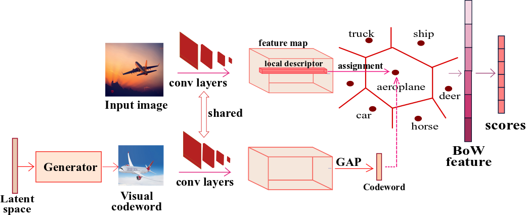
Figure 1: Interpretable BoW networks. We use a GAN to generate a visual codebook, from which we obtain the codewords of a BoW model. This allows us to associate a visual and semantic meaning to the codewords, and, as shown in our experiments, to detect adversarial samples by comparing the input image with the most highly activated visual codeword.

BoW-based representations, such as histograms [24, 43, 47], VLAD [22, 2] and Fisher Vectors [45, 42], have a longstanding history in the computer vision community. In the current deep learning era, they have been re-visited to yield novel, structured ways of pooling local activations into a global image representation [1, 49]. In essence, these strategies rely on measuring the distance between feature vectors and a codebook that is learnt jointly with the network parameters. Here, we argue that this distance-based representation is inherently interpretable; it allows one to understand the similarity between the input image and the codewords, which can be thought of as prototypes. However, in existing architectures, the codewords do not have a human-interpretable meaning, thus preventing one to visualize the reason behind the network’s prediction.

In this paper, we therefore introduce an approach to provide an interpretable meaning to the codebook of a BoW network. Specifically, we propose to associate a visual and semantic representation to each codeword. As illustrated in Fig. 1, this is achieved by making use of a generative adversarial network (GAN) [13, 44] that maps latent vectors to images. These images are then passed through the same base network as the one at the core of our BoW model, and we take the resulting feature vectors as our codebook elements. We then fine-tune the BoW model for classification with this codebook, which, in essence, allows it to learn a similarity between an input image and the images associated with the codewords. Ultimately, given a new image, observing the most highly activated codewords yields a visual and semantic interpretation of the network’s prediction.

As a second contribution, we propose to leverage our interpretable BoW networks to detect adversarial examples, that is, images to which a small amount of structured noise has been added so as to fool a pre-trained network. To this end, we rely on the intuition that an adversarial example (i) looks similar to the unaltered, but unknown, image; and (ii) to produce an erroneous prediction, will have a high activation for a codeword that corresponds to the wrong class. The image associated with this codeword, however, constitutes a prototype of this wrong class, and thus will look very different from the adversarial example itself. We therefore cast adversarial example detection as the problem of comparing the adversarial image with the visual representation of the most highly activated codeword.

Our experiments demonstrate that our interpretable BoW networks (i) yield visually and semantically meaningful representations; (ii) are more robust than traditional CNNs to adversarial examples; and (iii) yield codewords whose visual representation can be effectively exploited to detect adversarial examples and even out-of-distribution examples. In particular, our approach outperforms the state-of-the-art adversarial example detection methods on standard benchmarks for state-of-the-art attack strategies, such as CW [5], FGSM [14], and BIM [28]. We will make our code publicly available upon acceptance of the paper.

2 Related Work

BoW representations. Automatically recognizing objects in images and videos is central to a wide variety of application domains, such as security and autonomous driving. Visual recognition has therefore been one of the fundamental goals of computer vision since its inception. Prior to 2012, most methods followed a two-step pipeline comprised of handcrafted feature extraction from the images and separately training a classifier. Bags of visual Words (BoW) [24, 43, 47], that is, histograms extracted by comparing local features to the elements of a codebook obtained from the training data, quickly became popular handcrafted representations. They were then extended to VLAD [22] and Fisher Vectors [45, 42], which encode higher-order statistics of the data with respect to the codewords. After AlexNet’s impressive performance [27], much of the visual recognition research moved to employing deep networks. While most architectures extract the final image representation using standard convolutions, a few works attempted to leverage knowledge from the handcrafted features era. In particular, [12] exploits a VLAD pooling strategy on features extracted with a pre-trained network. While this separates feature extraction and classifier training, HistNet [52], NetVLAD [1], ActionVLAD [11], and Deep FisherNet [49] constitute end-to-end learning frameworks leveraging BoW, VLAD and Fisher Vector representations, respectively. Here, we contribute to this effort with a new deep architecture that incorporates the notion of interpretability in the BoW representation.

Interpreting CNNs. Attempts at interpreting the representations learned by CNNs or their predictions remain few, and existing methods follow two main trends. The first one [36, 35, 41, 55] focuses on visualizing the CNN filters in a post-training stage, by either inverting the network, or performing gradient ascent in image space to maximize neuron’s activations. The second trend consists of identifying the image regions that bear the most responsibility for the prediction. Note that this idea can be traced back to non-deep learning strategies, such as image representations based on object detectors [32] and classemes [50], and even part-based models [7, 8, 9]. In the deep learning context, this was introduced by [57], extended in [46], both of which use a post-training strategy. This was followed by [51] that incorporates an attention module at every layer of the network. In [56], an additional loss function was designed to assign each CNN filter to an object part. Recently [10, 39] have proposed to leverage attention maps during pooling operations. In this paper, we introduce an alternative way to interpret the prediction of a CNN by providing a visual and semantic representation to the codewords of a BoW model. While [39] also relies on a histogram-based representation, their approach differs fundamentally from ours, in that it does not assign a visual interpretation to the codebook.

Adversarial attacks and detection. When the sensitivity of deep networks to adversarial attacks was identified [48], initial works focused on developing defense strategies [14, 28], aiming to robustify the networks. However, these defenses were typically found to be vulnerable to optimization-based techniques [5]. Therefore, the research focus has increasingly shifted towards detecting adversarial samples, thus allowing one to discard them instead of attempting to be robust to them. In this context, [37] proposed to use a separate subnetwork to detect adversarial examples; [16] relies on knowledge distillation and Bayesian uncertainty to train a simple logistic regression detector; [34] exploits a measure of local intrinsic dimensionality to identify the adversarial examples. Here, we show that we can outperform all these methods by learning to compare the input image with the visual representation of the most highly activated codeword in our interpretable BoW network.

Another problem related to adversarial sample detection is that of identifying out-of-distribution (OOD) examples. This task has been addressed by training a detector on the softmax scores of a network [21], extended in [33] by an additional pre-processing of the network input. The contemporary work [31] introduced a unified framework for adversarial and OOD sample detection based on the Mahalanobis distance between hidden features and their class-conditional distributions. Here, unlike existing methods, we base our adversarial and OOD detection framework directly on a visual and semantic interpretation of the network’s prediction. This, we believe, would further give one the possibility to visually analyze the successful attacks, opening the door to human intervention in the detection process, while facilitating the human’s task.

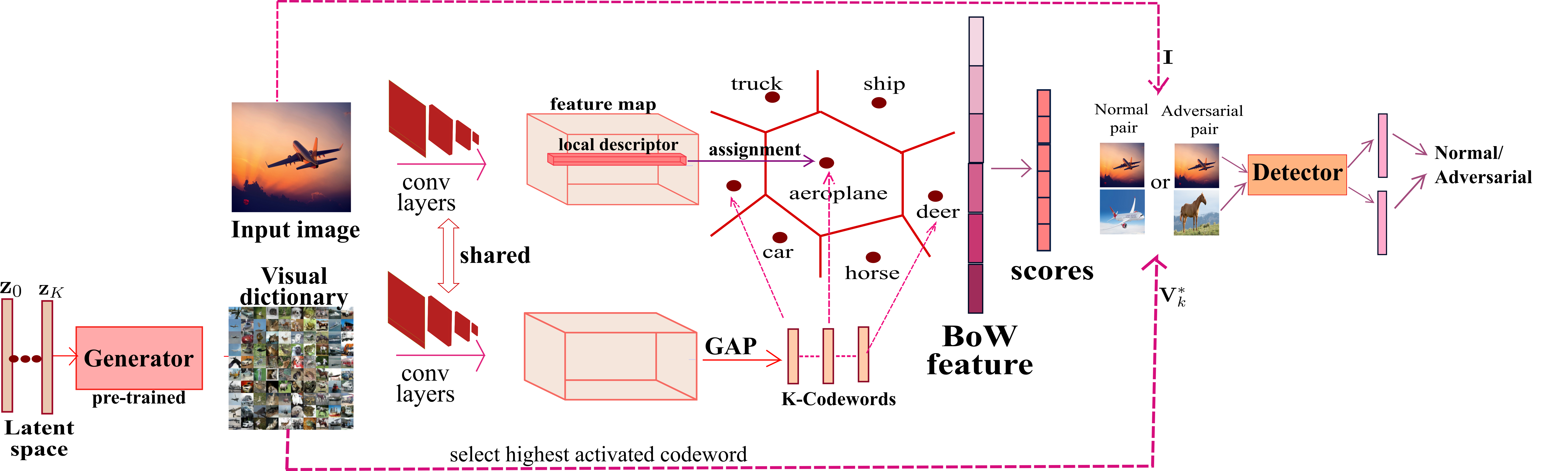
Figure 2: Interpretable BoW network for adversarial sample detection. An input image is passed through the network, and we retrieve the visual codeword with highest activation. We then pass these two images through a two-stream model which compares them using the Euclidean distance in feature space, so as to determine if they belong to the same class.

3 Method

In this section, we first introduce our interpretable BoW networks. We then show how to use the resulting visual codebook as a cue to detect adversarial and out-of-distribution (OOD) samples.

3.1 Interpretable BoW Networks

Typically, deep neural networks aggregate the local features of the convolutional maps, including the last one, using average or max pooling, which does not separately account for the contributions of the individual image regions. By contrast, here, we aim to leverage a BoW representation, where these individual contributions are preserved by comparing each local feature to the elements of a codebook. More specifically, we draw our inspiration from the histogram-based models of [52, 1, 49], but propose to provide an interpretable representation of the codebook. Below, we first formalize the BoW network, and then introduce our interpretable representation.

BoW network. Formally, let $\mathbf{I}$ be an image input to a CNN, and $\mathbf{X}\in\mathbb{R}^{W\times H\times D}$ be the feature map output by the CNN’s last convolutional layer, with spatial resolution $W\times H$ and $D$ channels. $\mathbf{X}$ can be thought of as $M=W\cdot H$ local descriptors $\mathbf{x}_{i}$ of dimension $D$. We then introduce a BoW layer that, given a codebook $\mathbf{B}$ with $K$ codewords, produces a $K$-dimensional representation of the form

$$\mathbf{h}(\mathbf{X})=\frac{1}{M}\sum_{i=1}^{M}\mathbf{h}_{i}(\mathbf{x}_{i})\;,$$ (1)

which aggregates local histogram-like vectors for each feature $\mathbf{x}_{i}$. We express these local vectors as

$$\mathbf{h}_{i}(\mathbf{x}_{i})=[a_{0}(\mathbf{x}_{i}),a_{1}(\mathbf{x}_{i}),\cdots,a_{K}(\mathbf{x}_{i})]^{T}\;,$$ (2)

where $a_{k}(\mathbf{x}_{i})$ is given by

$$a_{k}(\mathbf{x}_{i})=\frac{e^{-\alpha\left\|\mathbf{x}_{i}-\mathbf{b}_{k}\right\|^{2}}}{\sum_{k^{\prime}}{e^{-\alpha\left\|\mathbf{x}_{i}-\mathbf{b}_{k^{\prime}}\right\|^{2}}}}\;.$$ (3)

This value represents the assignment of descriptor $\mathbf{x}_{i}$ to codeword $\mathbf{b}_{k}$. Note that, in the classical BoW formalism, the assignments are binary, with each descriptor being assigned to a single codeword. Within a deep learning context, for differentiability, we relax them as soft assignments, with $\alpha$ a hyper-parameter defining the softness. The resulting BoW vector $\mathbf{h}(\mathbf{X})$ then acts as input to the final classification layer of the network.

To obtain the codebook $\mathbf{B}$, one typically first trains the base network, with global average pooling (GAP) of $\mathbf{X}$ and a softmax classifier, and then performs $K$-means clustering on the local features $\{\mathbf{x}_{i}\}_{i=1}^{M}$ of all training samples [1, 49]. Since the codebook is then defined over abstract features, it does not have a clear visual or semantic meaning. Here, we propose to provide the codebook with such a meaning, which then translates to making our BoW network interpretable; given an input image $\mathbf{I}$, one can analyze the prediction by visualizing the representation of the most highly activated codeword.

Providing interpretability. To obtain a visual and semantic codebook representation, we propose to exploit the generator of a pre-trained GAN. As illustrated in Fig. 1, the images obtained from this generator are passed through the same base network as that of our BoW model, and the resulting average-pooled features taken as codewords. As a result, the set of $K$ generated images $\{\mathbf{V}_{k}\}_{k=1}^{K}$ can be thought of as a visual dictionary, and each codeword $\mathbf{b}_{k}$ in the codebook $\mathbf{B}$ is directly associated to a visual interpretation $\mathbf{V}_{k}$. As GANs are now able to generate diverse images that cover all the classes in a dataset, this visual interpretation inherently comes with a semantic meaning.

Given an input image $\mathbf{I}$, with corresponding final feature map $\mathbf{X}$, we can obtain an interpretation of its prediction by observing the visual codeword $\mathbf{V}_{k^{*}}$ associated to the most highly activated codeword, that is,

$$k^{*}=\operatornamewithlimits{argmax}_{k}\mathbf{h}^{k}(\mathbf{X})\;,$$ (4)

where $\mathbf{h}^{k}(\mathbf{X})$ denotes the $k^{th}$ element of the vector $\mathbf{h}$ in Eq. 1. For a sample from class $c$, this visual codeword will typically correspond to an image of the same class. It will, moreover, depict characteristics similar to that of the input image, and, as shown in our experiments, different codewords from the same class $c$ will focus on different characteristics, thus truly acting as prototypes.

Training. In principle, our model can be trained in an end-to-end manner. We found, however, that training all the different parts jointly from scratch was unstable. To overcome this, we rely on the following training strategy. We first pre-train the GAN on the training images of the dataset of interest, and train the base network of our BoW model using average pooling with a standard softmax classifier. We then compute an initial codebook $\mathbf{B}_{0}$ via $K$-means clustering of the average-pooled features of the last convolutional layer of this base network. Specifically, we define an equal number of codewords $S$ for each class. Thus, for a $C$-class dataset, we obtain $K=CS$ codewords, and force each group of $S$ codewords to come from the same class during the clustering procedure. Note that this further encodes the notion of semantic meaning of each codeword.

To obtain a visual representation of each codeword in $\mathbf{B}_{0}$, we optimize the input $\mathbf{z}$ of the generator, whose weights are fixed, so as to generate an image that, when passed through the base network, yields features that are close to the codeword in the least-square sense. That is, formally, for each codeword $\mathbf{b}_{0,k}$ in $\mathbf{B}_{0}$, we solve

$$\mathbf{z}^{*}_{k}=\operatornamewithlimits{argmin}_{\mathbf{z}}\|f(g(\mathbf{z}))-\mathbf{b}_{0,k}\|^{2}\;,$$ (5)

where $g(\cdot)$ represents the generator, and $f(\cdot)$ the base network up to the last average pooling operation. We then take our codebook $\mathbf{B}$ to be the set of generated features $\{f(g(\mathbf{z}^{*}_{k}))\}$, and train our BoW model by replacing the base network classification layer with a layer that maps the BoW representation to the class labels and using the standard cross-entropy loss.

Note that, while this training procedure may seem costly, this has no effect on the computational cost at test time. Indeed, inference only involves a forward pass through our BoW network, which, compared to the base network, only requires us to store the additional codebook $\mathbf{B}$; that is, the generator network is not needed anymore.

3.2 Detecting Adversarial Examples

By providing a visual and semantic meaning related to the network’s prediction, our interpretable BoW network can be leveraged to detect adversarial examples. The reasoning behind this is the following: Typically, adversarial attacks aim to add the smallest amount of perturbation to an image so that the network misclassifies it. While this perturbation should be imperceptible to humans, it should strongly affect the resulting deep representation. In our case, this representation is the BoW one, and, for misclassification to occur, the most highly activated codeword should typically be associated to the wrong class. As such, its visual representation should look significantly different from the adversarial example. We therefore propose to train an adversary detector network that, given two input images, predicts whether they belong to the same class or not.

Formally, our detection framework, depicted by Fig. 2, proceeds as follows. An image $\mathbf{I}$, adversarial or not, is passed through our interpretable BoW network, and we retrieve the visual codeword $\mathbf{V}_{k^{*}}$ corresponding to the highest activation using Eq. 4. We then pass $\mathbf{I}$ and $\mathbf{V}_{k^{*}}$ to our adversary detector, which outputs a binary label indicating whether the two images belong to the same class or not. If they don’t, then $\mathbf{I}$ is detected as an adversarial example.

Our detector is a two-stream network that extracts features for the two images independently. To train this network, we make use of the contrastive loss [19] , which aims to make the Euclidean distance between pairs of mismatched images larger than a margin $m=1$, while minimizing that of matching pairs. Detection is then performed by comparing the Euclidean distance to the margin.

While, in our experiments, we train the detector to identify adversarial examples, it can also be used to detect OOD samples, even without any re-training. In essence, the intuition remains unchanged: An OOD sample will activate a codeword whose visual representation looks different from the input image. The detection procedure is thus the same as in the case of adversarial examples.

4 Experiments

We now empirically evaluate our interpretable BoW networks. To this end, we first analyze the semantic meaning of the learned visual dictionaries. We then demonstrate their benefits to detect adversarial and out-of-distribution samples. In these experiments, we used the standard benchmark datasets employed for adversarial sample detection, that is, MNIST [30], F-MNIST [53], CIFAR-10 [25], SVHN [40].

Implementation details. For our comparisons to be meaningful, we rely on the same base architecture as in [34] on each dataset. This architecture is first trained with a softmax classifier for 50-100 epochs and used to compute the initial codebook $\mathbf{B}_{0}$. In parallel, we train either a GAN [13] or a WGAN [18], depending on the dataset, for 100k iterations. From the resulting generator and $\mathbf{B}_{0}$, we obtain our interpretable codebook $\mathbf{B}$ following the procedure described in Section 3.1. We then train the classification layer of our interpretable BoW model for $40$ epochs.

In all our experiments, we set $\alpha=100$ in the BoW soft-assignment policy of Eq. 3, and use the Adam [23] optimizer with a learning rate of 0.001 and a decay rate of 0.1 applied every 20 epochs. Due to space limitation, we provide the detail of the base classifier and the GAN architecture in the supplementary material. The test errors on MNIST, FMNIST, CIFAR-10, and SVHN using the softmax classifier and the BoW one are given in Table 1. In essence, both classifiers perform on par. Note that our goal here is not to advocate for superior performance of the BoW model, but rather for its use to provide a visual interpretation, as discussed below.

Dataset	Base network	BoW network
MNIST	99.23	99.15
FMNIST	92.46	92.06
CIFAR-10	87.54	87.95
SVHN	92.43	91.81

Table 1: Classification accuracy (in %) of the base and BoW networks. Note that both models perform on par, but the BoW one allows us to obtain a visual interpretation.

4.1 Visualizing BoW Codewords

Each codeword in our BoW model is directly associated with an image generated by a GAN. In Fig. 3, we visualize these images for MNIST, FMNIST, SVHN and CIFAR-10. Zooming in on the figure confirms that the learned codebooks nicely cover the diversity of the classes in these datasets. For example, in FMNIST, each garment appears in a variety of sizes and styles. Similarly, in CIFAR-10, each object appears in different colors, orientations and in front of different backgrounds. Furthermore, and more importantly, each one of these images retains the semantic meaning of the class label for which it was generated. This will prove key to the success of our adversarial sample detector, as discussed in the next section.

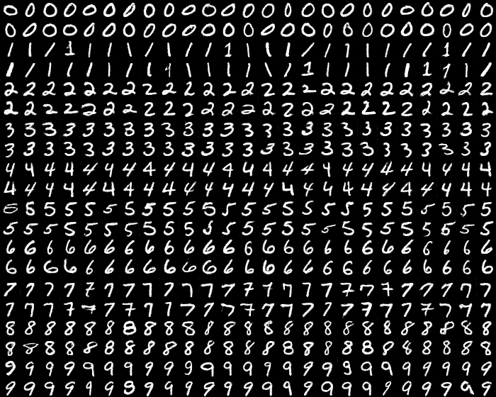
(a) MNIST codewords

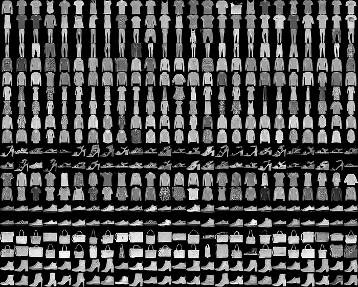
(b) FMNIST codewords

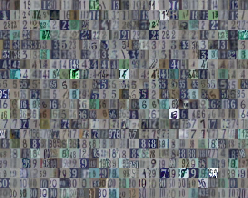
(c) SVHN codewords

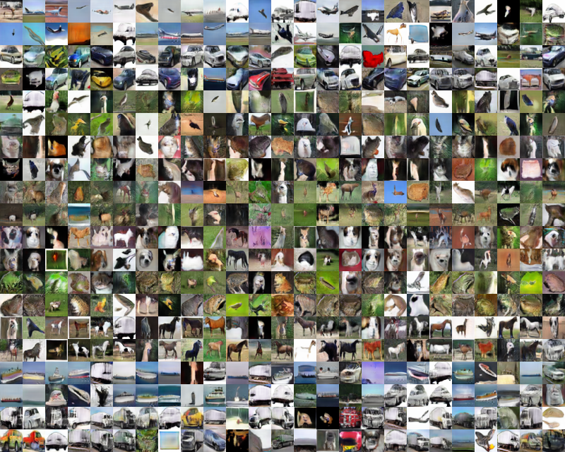
(d) CIFAR-10 codewords

Figure 3: Visual interpretations of the BoW codebooks. Every two rows correspond to one class. Note that these codewords capture the diversity of the classes in each dataset (better seen by zooming in).

In the top row of Fig. 4, we show the codewords with highest activation for a few correctly-classified images of each dataset. Note that, in most cases, the corresponding codeword has the same semantic meaning as the input image, not only because it corresponds to the same class, but also because it depicts a visually similar content, e.g., in terms of color and orientation. More such visualizations are provided in the supplementary material.

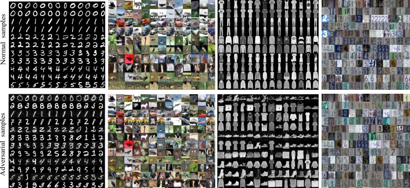
Figure 4: Visualization of the most highly activated codeword for normal and adversarial samples. Each two rows within a block show the input image (top) and corresponding codeword (bottom). The adversarial examples were obtained with a BIM-a attack. Additional visualizations for other datasets and attacks are provided in the supplementary material.

4.2 Adversarial Attacks

We make use of the state-of-the-art attack methods, FGSM [14], BIM-a [28], BIM-b [28], DeepFool [38] and CW [5], to evaluate (i) the robustness of our interpretable BoW model to adversarial samples; and (ii) the effectiveness of our detection strategy. In both cases, following common practice [34], we discard the images that were misclassified by the original networks from this evaluation.

To first validate our intuition that adversarial samples will activate codewords corresponding to the wrong classes, and that these codewords will be visually dissimilar to the input image, in the bottom row of Fig. 4, we provide the most highly activated codeword images for a few successful adversarial attacks. Note that these images are indeed semantically and visually different, which will facilitate the task of our detector.

4.2.1 Robustness of Interpretable BoW Networks

Before evaluating the effectiveness of our detection strategy, we study the robustness of our BoW model to the adversarial attacks. In particular, we focus on white-box attacks, where the attacker has access to the exact model it aims to fool. There are two ways to attack our BoW model: One can generate adversarial examples either for the BoW model itself, or for the base network. We refer to the latter as transferred BoW (T-BoW) attacks. In Table 2, we compare the success rates of different attack strategies on our BoW model with those on the base network. Note that attacks directly targeting our BoW model are significantly less successful than those on the base network. While transferring the adversarial samples of the base model to our BoW network is more effective than the direct attacks, the success rates remain lower than on the base model. Note that, as shown in the supplementary material, the $L_{2}$ norm of the perturbations was similar for all network settings. This, we believe, shows that our BoW models are more robust than traditional networks to adversarial attacks. Nevertheless, some attacks are successful, and we now turn to the problem of detecting them.

Dataset	Model	FGM	BIM-a	BIM-b	CW
MNIST	Base	93.68	100.0	100.0	100.0
	T- Bow	92.70	38.94	100.0	31.40
	BoW	39.23	23.96	23.96	3.9
F-MNIST	Base	99.64	100.0	100.0	100.0
	T- Bow	98.80	65.52	100.0	49.08
	BoW	57.78	32.09	31.97	66.78
SVHN	Base	97.0	100.0	100.0	100.0
	T- Bow	96.83	93.77	100.0	75.24
	BoW	73.39	73.11	72.24	86.42
CIFAR-10	Base	82.70	97.10	97.10	100.0
	T- Bow	82.66	94.12	97.15	76.92
	BoW	60.66	94.18	93.93	99.99

Table 2: Success rates of white-box attacks on the base network and on our BoW network. Note that, whether attacked directly (BoW) or via the base network (T-BoW), our model is more robust to adversarial attacks.

4.2.2 Detecting Adversarial Samples

Adversarial detector. We now evaluate the effectiveness of the detection strategy introduced in Section 3.2. To this end, we train our detector using adversarial examples generated by the white-box attacks discussed above. Specifically, we report results obtained with two training strategies. Strategy 1, which is commonly used [34], consists of defining a balanced training set comprised of normal images (positives) and their adversarial counterparts (negatives). A drawback of this strategy, however, is that, as shown above, many attacks are unsuccessful with our BoW model, and considering such samples as negatives essentially adds noise to our training process, since unsuccessful adversarial samples will typically activate a codeword that is similar to the input image. To overcome this, we therefore propose Strategy 2, which consists of using only the successful adversarial examples as negatives during training. The resulting training set, however, is then imbalanced. The detailed detector architectures are provided in the supplementary material.

Comparison with the state of the art. We compare our approach with the state-of-the-art BU [17] and LID [34] methods, which have proven more robust than the earlier detection strategy [6]. In Table 3, we report the area under the ROC curve (AUROC) for BU, LID and our method, using both Strategy 1 and Strategy 2. In this case, the results were obtained using the adversarial examples generated with a white-box attack on our BoW model directly. As such, BU and LID were also applied to our BoW model. Note that we outperform the state of the art in all but one case, by a particularly large margin when the results are not already saturated, such as with BIM-a on SVHN and CIFAR-10 and with FGSM on CIFAR-10. The only case where we don’t is with CW on MNIST, with Strategy 1. Note, however, that, as shown in Table 2, in this case, CW only has a 3.9% success rate. This results in Strategy 1 having access to very few training samples. By contrast, with Strategy 2, we outperform the baselines for the CW attack by a large margin. In Table 4, we provide similar results for attacks targeted to the base network. The conclusions are the same: We outperform the baselines in most cases, and by a large margin where there remained room for improvement.

Similarly to [34], we also evaluate whether our detector trained for one specific attack generalizes to other ones. In Table 5, we compare the generalizability of our approach and of LID. For each method, we show the results of the model that was trained on the attack that makes it generalize best to the other ones. Note that the performance of our detector is virtually unaffected. While LID also generalizes well, our method still outperforms it in most cases, and by a large margin in several scenarios.

Dataset	Feature	FGSM	BIM-a	BIM-b	CW
MNIST	KD+BU	95.22/94.11	82.54/72.80	82.17/72.43	50.17/60.01
	LID	92.66/91.18	82.24/61.90	83.06/75.61	51.81/68.46
	Ours	100.00/100.0	100.0/100.0	100.0/100.0	50.87/ 100.0
F-MNIST	KD+BU	99.33/99.36	91.35/87.32	89.43/85.39	69.68/65.83
	LID	93.88/93.93	86.95/81.06	86.83/81.11	73.23/70.84
	Ours	100.0/100.0	100.0/100.0	100.0/100.0	83.97/97.96
SVHN	KD+BU	78.21/74.24	78.37/73.97	67.96/71.46	88.68/88.62
	LID	99.88/99.25	83.45/84.17	85.76/90.42	91.23/91.40
	Ours	99.9/100.0	98.71/96.16	99.9/100.0	96.52/96.49
CIFAR-10	KD+BU	72.79/69.66	86.23/85.69	60.23/62.52	93.74/93.74
	LID	89.67/89.26	85.40/85.02	80.55/82.79	93.57/93.17
	Ours	99.37/99.97	93.90/97.47	99.90/99.96	96.52/96.35

Table 3: AUROC scores for BU, LID and our detector for direct BoW attacks. Left and right numbers correspond to Strategy 1 and Strategy 2, respectively.

Dataset	Feature	FGSM	BIM-a	BIM-b	CW
MNIST	KD+BU	93.73/93.63	86.09/83.09	79.22/79.22	80.64/80.64
	LID	99.17/99.15	99.75/99.75	95.16/96.16	99.01/99.03
	Ours	100.00/100.0	100.0/100.0	100.0/100.	99.85/100.0
F-MNIST	KD+BU	96.99/97.03	92.60/92.60	97.74/97.74	93.27/93.27
	LID	95.68/95.68	95.95/95.95	95.24/95.24	97.31/97.31
	Ours	100.0/100.0	99.98/100.0	100.0/100.0	98.26/97.96
SVHN	KD+BU	85.04/85.08	88.06/88.06	99.99/99.99	92.85/92.85
	LID	99.88/99.32	88.45/84.17	98.76/99.93	94.23/94.23
	Ours	99.99/100.0	96.66/96.25	100.0/100.0	95.61/96.86
CIFAR-10	KD+BU	75.75/74.67	80.02/79.69	99.12/99.24	96.06/96.05
	LID	87.16/87.92	82.17/81.77	99.91/99.91	97.54/97.56
	Ours	99.80/99.71	96.77/96.87	99.77/99.85	96.70/97.24

Table 4: AUROC scores for BU, LID and our detector for attacks on the base network. Left and right numbers correspond to Strategy 1 and Strategy 2, respectively.

Dataset	Method	Train	FGSM	BIM-a	BIM-b	CW
MNIST	LID	FGSM	91.18	65.48	64.42	29.05
	Ours	BIM-a	100.0	100.0	100.0	97.56
F-MNIST	LID	FGSM	93.88	82.24	82.58	65.03
	Ours	CW	97.39	97.13	95.85	97.96
SVHN-10	LID	FGSM	99.25	77.54	79.77	75.16
	Ours	BIM-a	91.41	96.25	91.30	94.73
CIFAR-10	LID	FGSM	89.26	66.55	68.33	66.05
	Ours	BIM-a	86.90	97.47	95.02	95.44

Table 5: Generalizing to different attacks. We compare the results of LID and our detector in the scenario where the detectors were trained for a specific attack, but tested on different ones. These results were obtained with Strategy 2.

4.3 Attacking the Detector

In the previous set of experiments, we have worked under the assumption that the attacker only had access to our BoW model, but not to the detector. Here, we remove this assumption, and study two more challenging scenarios. In the first one, the attacker knows our detection strategy, but not the model we use. In the second, the attacker also has access to our detector.

4.3.1 Adaptive Attack

To evaluate the robustness of our approach in the scenario where the attacker is aware of our detection scheme, we apply an adaptive CW attack strategy similar to the ones used in [4, 34] to attack the KD & LID detectors, respectively. To this end, we modify the objective of the CW attack as

$$\arg\min_{\mathbf{I}_{adv}}\left\|(\mathbf{I}-\mathbf{I}_{adv}\right\|_{2}^{2}+\alpha\cdot\big{(}\ell(\mathbf{I}_{adv})+\left\|\phi(\mathbf{I})-\phi(\mathbf{I}_{adv})\right\|_{2}^{2}).$$ (6)

The first two terms correspond to the original CW attack, with $\alpha$ balancing the amount of perturbation and the adversarial strength, that is, how strongly one forces the adversarial image to be misclassified. The last term directly reflects our detection strategy and encourages the BoW representation of the real, $\phi(\mathbf{I})$, and adversarial, $\phi(\mathbf{I}_{adv})$, images to be similar. The rationale behind this is that the attack then aims to find an adversarial perturbation such that the sample is not only misclassified, but also has a representation close to that of the real image, thus breaking the premise on which our detector is built.

Dataset	Attack success rate	Detector AUROC
F-MNIST	33.11	96.22
SVHN	94.58	96.54
CIFAR-10	99.95	97.47

Table 6: Adaptive attacks. Our detector remains robust to an attacker that knows our detection strategy.

In Table 6, we report both the success rate of this adaptive attack on our BoW model and the AUROC of our detector, trained with Strategy 2. Note that our detector still yields high AUROC, thus showing that it remains robust to an attacker that knows our detection strategy.

4.3.2 White-box Detector Attacks

We now evaluate the robustness of our method in the case where the attacker has access to all our models, that is, the BoW model, the GAN and the adversarial sample detector. Note that access to the parameters of the generator and detector networks is not a mild assumption since information about the training data is required to compute them.

To attack our complete framework, we generate adversarial images $\mathbf{\mathbf{I}}_{adv}$ in a two-step fashion. First, we attack the BoW classifier to generate an intermediate adversarial image $\mathbf{I}_{adv}^{0}$ that activates codeword $j$ corresponding to image $\mathbf{V}_{j}$ in the visual codebook. Second, we attack the detector to misclassify $\mathbf{V}_{j}$ as being similar to the input image. Since our detector relies on the distance between the input image and the codeword in feature space, fooling it can be achieved by finding a perturbation that solves the optimization problem

$$\min_{\mathbf{I}_{adv}}\left\|\mathbf{I}_{adv}^{0}-\mathbf{I}_{adv}\right\|_{2}^{2}+\alpha\cdot\left\|\gamma(\mathbf{V}_{j})-\gamma(\mathbf{I}_{adv})\right\|_{2}^{2}\;,$$ (7)

where $\gamma(\cdot)$ is the feature-extraction part of our detector.

Dataset	Classifier	Detector	Attack success rate	Attack success rate on detector
	attack	attack	on detector	trained with adversarial training
MNIST	FGSM	FGSM	0.00	0.0
	CW	CW	100.00	8.0
F-MNIST	FGSM	FGSM	2.8	0.0
	CW	CW	100	27.2

Table 7: White-box detector attacks. An attacker that has access to our BoW network, GAN and detector can indeed be successful when using the CW attack, but not the FGSM one. However, adversarial training allows us to robustify our approach to these attacks, as shown in the right column.

We found that, as is, our detector is indeed vulnerable to such an attack. To circumvent this, we therefore rely on the adversarial training strategy of [15], in which the detector is trained using dynamically-generated adversarial images. We observed that, after a few epochs of such dynamic training, our detector becomes robust to these white-box attacks. To evidence this, in Table 7, we provide the results of a white-box attack on a detector dynamically trained on limited balanced set of 10K samples and evaluated on 1K samples. These results show that our approach has become much more robust to this attack.

4.4 Detecting Out-of-distribution Samples

We now evaluate the use of our approach to detect OOD samples. Following the setup of [21], we perform experiments using either SVHN [40] or MNIST [25] as training datasets from which the in-distribution samples are drawn. The goal then is to detect OOD samples coming from other datasets, such as LSUN [54], TinyImageNet [26], Omniglot [29], Not-MNIST [3]. We consider two settings: In the first, the detection method does not see any OOD samples during training, but has access to adversarial examples generated by the BIM-a attack; in the second, the detector has access to 1000 images from the OOD dataset. In Table 8, we compare the results of our approach with those of the baseline method [21] and of ODIN [33]. Note that we clearly outperform them, both when we see OOD samples during training and in the more realistic case where we don’t. We believe that this demonstrates the generality of our approach.

In-Dataset	In-Dataset	Adversarial examples	OOD samples
		Baseline [21] / Ours
SVHN	CIFAR-10	87.44/97.26	87.92/99.14
	LSUN	89.06/99.87	89.06/99.98
	TinyImageNet	89.97/99.76	89.97/99.93
MNIST-10	Not-MNIST	77.11/97.44	77.23/99.98
	OMNIGLOT	82.11/97.01	82.24/100.0
	CIFAR	79.84/99.21	79.84/100.0

Table 8: Detecting OOD samples. We compare our detector with the baseline method of [21] and with the recent ODIN [33] one in the case where we only observe adversarial samples during training (left) and when we have access to a few OOD samples (right).

5 Conclusion

We have introduced a novel approach to interpreting a CNN’s prediction, by providing the elements in a BoW codebook with a visual and semantic meaning. We have then proposed to leverage the visual representation of these interpretable BoW networks for adversarial example detection. Our experiments have evidenced that (i) our interpretable BoW networks are more robust to adversarial attacks; (ii) our adversary detection strategy outperforms the state-of-the-art ones; (iii) our approach could be made robust to adversarial attacks to the detector itself; (iv) our framework generalizes to OOD sample detection. In the future, following the intuition that complex scenes and objects can be modeled as sets of parts, we plan to extend our interpretable BoW representation to part-based ones. This, we believe, will also translate to improved adversary detection performance, since it will allow us to robustly combine the decision of each part.

6 Conclusion

We have introduced a novel approach to interpreting a CNN’s prediction, by providing the elements in a BoW codebook with a visual and semantic meaning. We have then proposed to leverage the visual representation of these interpretable BoW networks for adversarial example detection. Our experiments have evidenced that (i) our interpretable BoW networks are more robust to adversarial attacks; (ii) our adversary detection strategy outperforms the state-of-the-art ones; (iii) our approach could be made robust to adversarial attacks to the detector itself; (iv) our framework generalizes to OOD sample detection. In the future, following the intuition that complex scenes and objects can be modeled as sets of parts, we plan to extend our interpretable BoW representation to part-based ones. This, we believe, will also translate to improved adversary detection performance, since it will allow us to robustly combine the decision of each part.

Below, we provide additional details regarding our architectures and our experimental results.

7 Architectures

As base networks for our models, we used the same architectures as in [34]. These architectures are provided in Table 9 for the MNIST, FMNIST experiments, in Table 10 for SVHN experiments and in Table 11 for the CIFAR-10 experiments. For the detector in our adversarial example detection approach, we used the architecture shown in Table 12 for all datasets, except for CIFAR-10. In this case, we used a ResNet-20 [20] due to the higher image variance and background complexity of this dataset.

We also trained a GAN [13] for MNIST and FMNIST and a WGAN [18] for SVHN and CIFAR-10. The architectures of the generator for MNIST and FMNIST are provided in Table 13 and in Table 15 for SVHN and CIFAR-10. Similarly, the discriminator for MNIST and FMNIST is provided in Table 14 and the one for SVHN and CIFAR-10 in Table 16.

Layer	Parameters
Convolution + ReLU	$5\times 5\times 64$
Convolution + ReLU	$5\times 5\times 64$
MaxPool	$2\times 2$
Dense + ReLU	128
Softmax	10

Table 9: Base network for MNIST, FMNIST.

Layer	Parameters
Convolution + ReLU	$3\times 3\times 64$
Convolution + ReLU	$3\times 3\times 64$
MaxPool	$2\times 2$
Convolution + ReLU	$3\times 3\times 128$
Convolution + ReLU	$3\times 3\times 128$
MaxPool	$2\times 2$
Dense + ReLU	512
Dense + ReLU	128
Softmax	10

Table 10: Base network for SVHN.

Layer	Parameters
Convolution + ReLU	$3\times 3\times 32$
Convolution + ReLU	$3\times 3\times 32$
MaxPool	$2\times 2$
Convolution + ReLU	$3\times 3\times 64$
Convolution + ReLU	$3\times 3\times 64$
MaxPool	$2\times 2$
Convolution + ReLU	$3\times 3\times 128$
Convolution + ReLU	$3\times 3\times 128$
MaxPool	$2\times 2$
Dense + ReLU	1024
Dense + ReLU	512
Softmax	10

Table 11: Base network for CIFAR-10.

Layer	Parameters
Convolution + ReLU	$5\times 5\times 32$
MaxPool	$2\times 2$
Convolution + ReLU	$5\times 5\times 64$
MaxPool	$2\times 2$
Fully Connected + ReLU	128
Fully Connected + ReLU	128

Table 12: Detector for MNIST, FMNIST and SVHN.

Layer	Parameters
Input noise, $\mathbf{z}\in\mathbb{R}^{128}$	Nil
Dense + ReLU	$128\times 4\times 4$
Deconvolution + ReLU	$5\times 5\times 128$
Deconvolution + ReLU	$5\times 5\times 64$
Deconvolution + Sigmoid	$5\times 5\times 1$

Table 13: Generator for MNIST and FMNIST

Layer	Parameters
Input image, $\mathbf{I}\in\mathbb{R}^{28\times 28}$	Nil
Convolution + LeakyReLU, stride=2	$5\times 5\times 64$
Convolution + LeakyReLU, stride=2	$5\times 5\times 128$
Convolution + LeakyReLU, stride=2	$5\times 5\times 256$
Fully Connected + ReLU	1

Table 14: Discriminator for MNIST and FMNIST

Layer	Parameters
Input noise, $\mathbf{z}\in\mathbb{R}^{128}$	Nil
Dense	$128\times 4\times 4$
ResBlock + Up	$128$
ResBlock + Up	$128$
ResBlock + Up	$128$
Convolution + Tanh	$3\times 3\times 3$

Table 15: Generator for SVHN and CIFAR-10 similar to the ones used in  [18]

Layer	Parameters
Input image, $\mathbf{I}\in\mathbb{R}^{32\times 32\times 3}$	Nil
ResBlock + Down	$128$
ResBlock + Down	$128$
ResBlock +Down + GAP	$128$
Dense	1

Table 16: Discriminator for SVHN and CIFAR-10 similar to the ones used in  [18]

8 Additional Results on Normal Samples

We visualize the learned codewords on various datasets in Fig. 5. We also provide additional visualizations of the activated visual codewords for normal samples of MNIST, FMNIST, SVHN and CIFAR-10 in Fig. 6. We further visualize the images assigned to a particular codeword in Figs. 7,  8,  9 and  10 for MNIST, FMNIST, SVHN and CIFAR-10 respectively. Finally, the misclassified normal samples for all datasets are shown in Fig. 11.

9 Adversarial Attack Implementations

We used the Cleverhans library to generate adversarial images following the same settings as in [34]. In Table 17, we report the mean $L_{2}$ perturbation of the adversarial images for different attack methods. Note that FGSM and BIM-b tend to yield larger perturbations than BIM-a and CW.

Dataset	Model	FGSM	BIM-a	BIM-b	CW
MNIST	Base	7.45	2.67	6.73	1.55
	BoW	8.01	3.30	3.45	0.04
F-MNIST	Base	4.61	1.01	4.07	0.90
	BoW	4.62	1.78	2.07	0.97
CIFAR-10	Base	2.74	0.46	2.12	0.35
	BoW	2.73	0.66	1.54	0.45
SVHN	Base	7.08	1.02	6.16	1.16
	BoW	7.09	1.75	3.48	1.52

Table 17: Mean $L_{2}$ perturbation of the adversarial images on the base and BoW networks with different attack strategies.

10 Influence of the Number of Codewords

We evaluate the influence of the hyper-parameter $K$ in Eq. 2 of the main paper, which defines the number of codewords in our BoW models.To this end, in Table 18, we report the detection AUROC for different values of $K$ with FGSM attack on various datasets with evaluation Strategy 2. Perhaps surprisingly, with as few as $K=50$ clusters (5 clusters per class), we still obtain high AUROCs.

$K$	50	100	500	1000
MNIST	99.95	100.0	100.0	100.0
FMNIST	100.0	100.0	100.0	100.0
SVHN	99.33	100.0	100.0	100.0

Table 18: Influence of $K$ on detection AUROC

11 Additional Results on Adversarial Samples

We also provide additional visualizations of activated visual codewords for adversarial samples of MNIST, FMNIST, SVHN and CIFAR-10 in Figs. 12, 13, 14 and 15, respectively.

(a) MNIST

(b) FMNIST

(c) SVHN

(d) CIFAR-10

Figure 5: Visual interpretations of the BoW codebooks. Every two rows correspond to one class. Note that these codewords capture the diversity of the classes in each dataset (better seen by zooming in.)

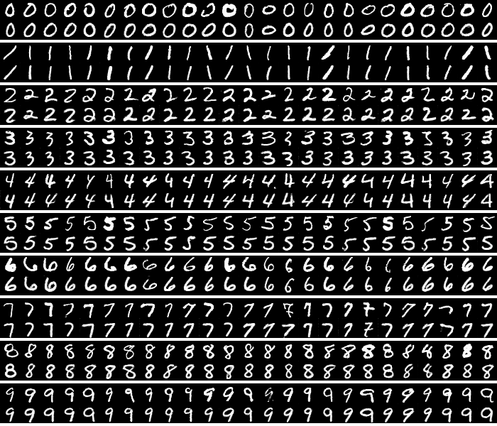
(a) MNIST

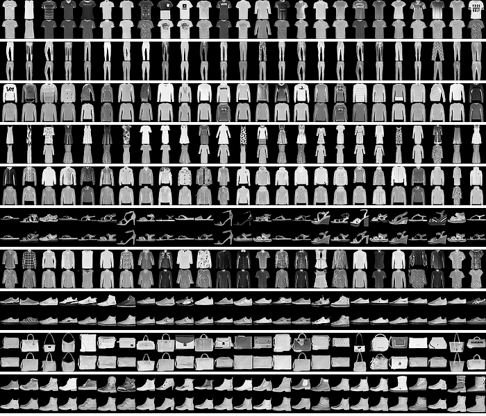
(b) FMNIST

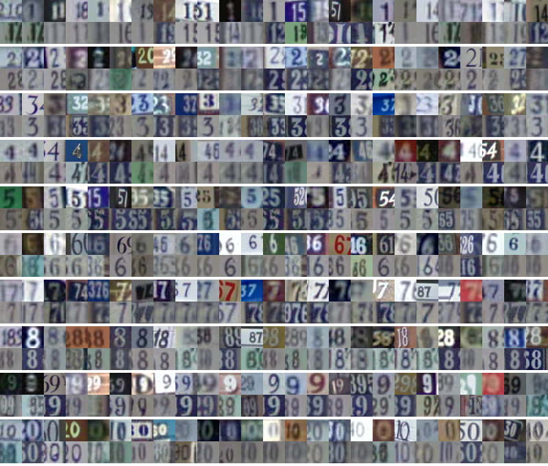
(c) SVHN

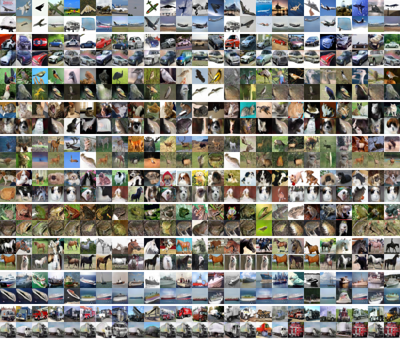
(d) CIFAR-10

Figure 6: Visualization of the most highly activated codeword for normal test samples. Each two rows within a block show the input image (top) and corresponding codeword (bottom).

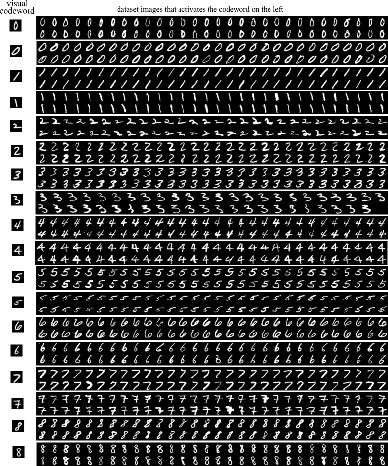
Figure 7: Dataset images from MNIST that activate a particular codeword. Each block has two columns. The left one shows the visual codeword and the right one the test images that activated the codeword on the left. Note that there is a clear semantic similarity between the images and the codeword, not only in terms of class label, but also with respect to style and orientation.

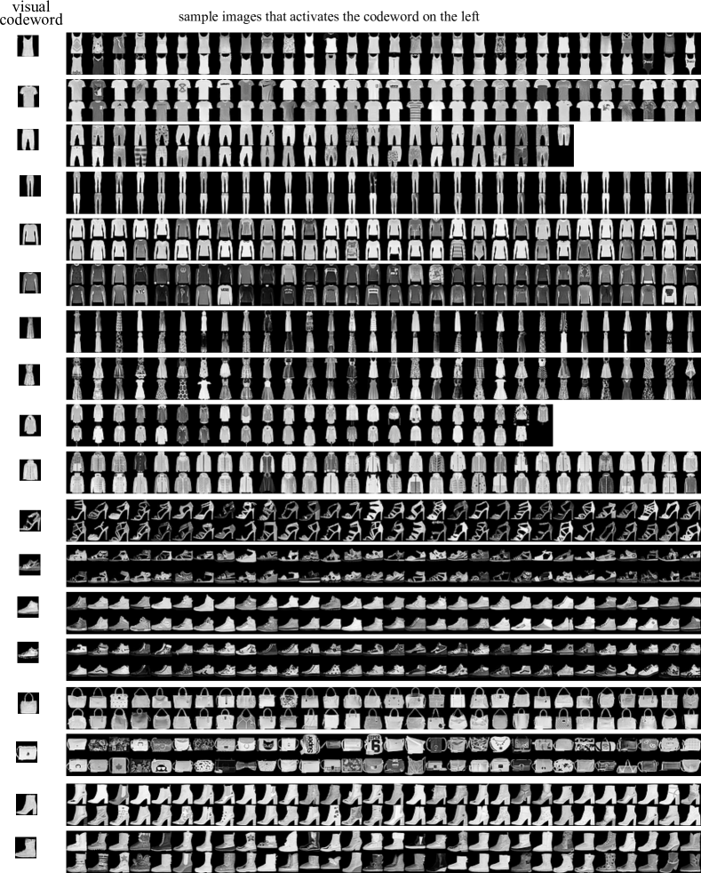
Figure 8: Dataset images from FMNIST that activate a particular codeword. Each block has two columns. The left one shows the visual codeword and the right one the dataset images that activated the codeword on the left. Note that there is a clear semantic similarity between the images and the codeword, not only in terms of class label, but also with respect to style and orientation.

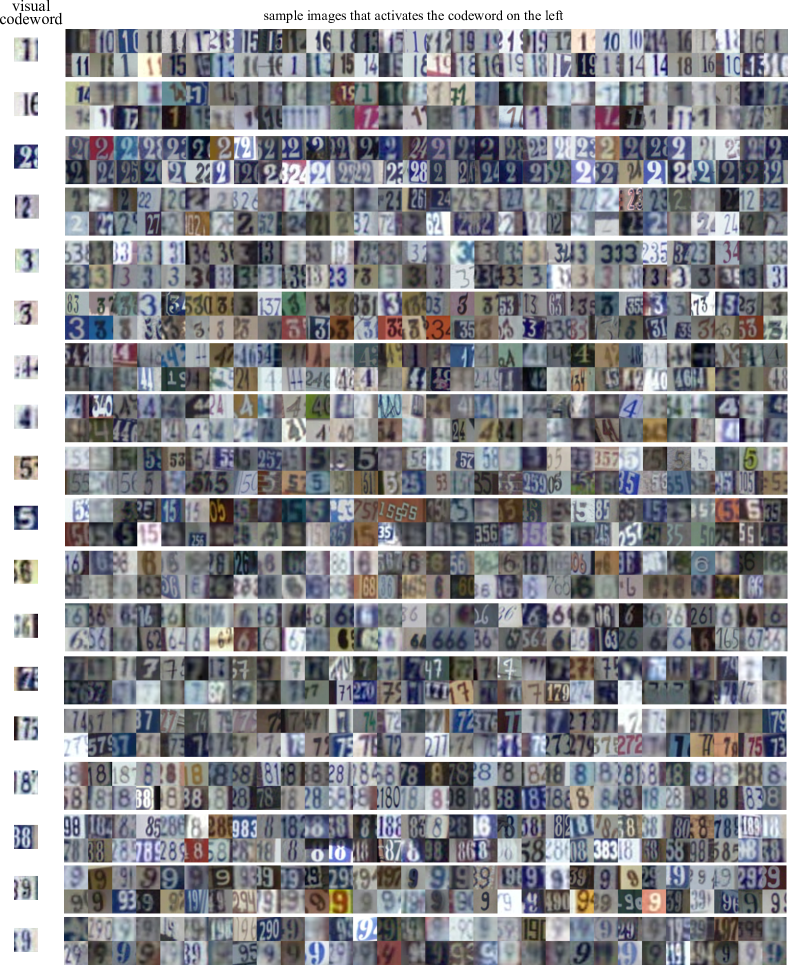
Figure 9: Dataset images from SVHN that activate a particular codeword. Each block has two columns. The left one shows the visual codeword and the right one the dataset images that activated the codeword on the left. Note that there is a clear semantic similarity between the images and the codeword, in terms of class label, but also with respect to style and orientation.

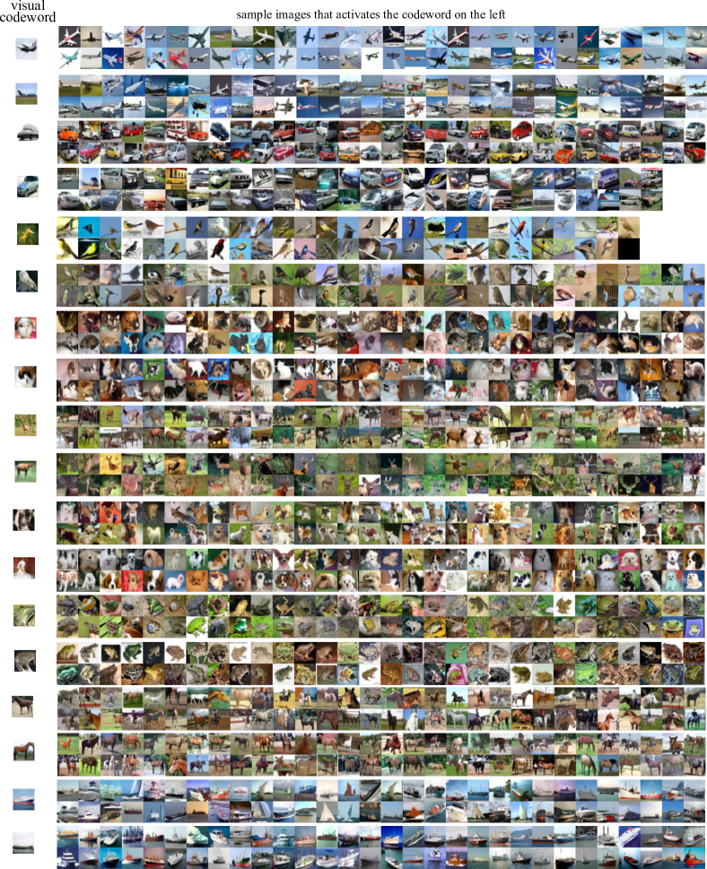
Figure 10: Dataset images from CIFAR-10 that activate a particular codeword. Each block has two columns. The left one shows the visual codeword and the right one the dataset images that activated the codeword on the left. Note that there is a clear semantic similarity between the images and the codeword in terms of class label.

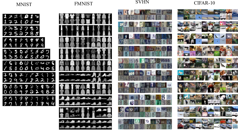
Figure 11: Most highly activated codewords of incorrectly classified test samples on various datasets. Each two rows within a block show the input image (top) of a specific class and the corresponding codeword (bottom). Note that the images and their codeword are dissimilar in most cases.

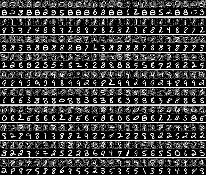
(a) FGSM

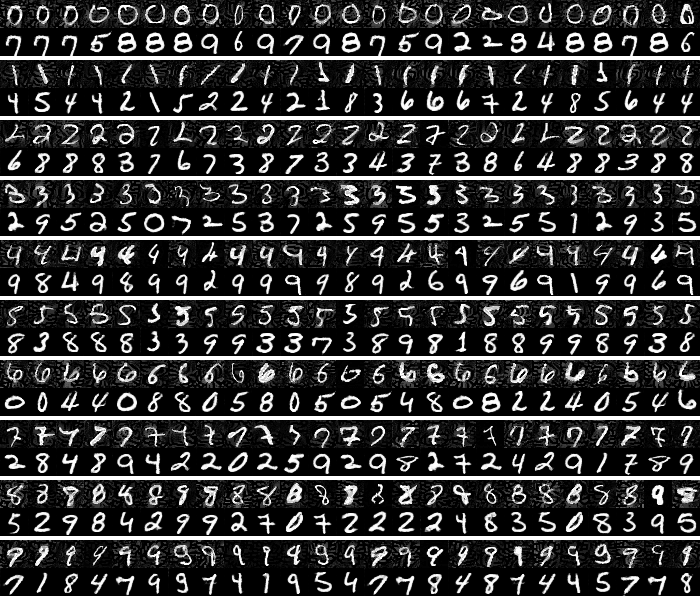
(b) BIM-a

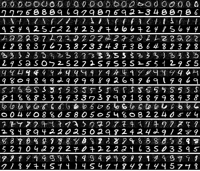
(c) BIM-b

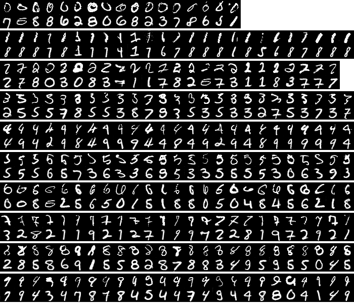
(d) CW

Figure 12: Most highly activated codewords of adversarial samples obtained with different attack strategies on MNIST test data. Each two rows within a block show the input image (top) and corresponding codeword (bottom). Note that the adversarial images and their codeword are dissimilar in most cases. Note that, in the CW case, we have fewer samples in some of the classes because of the low success rate of this attack.

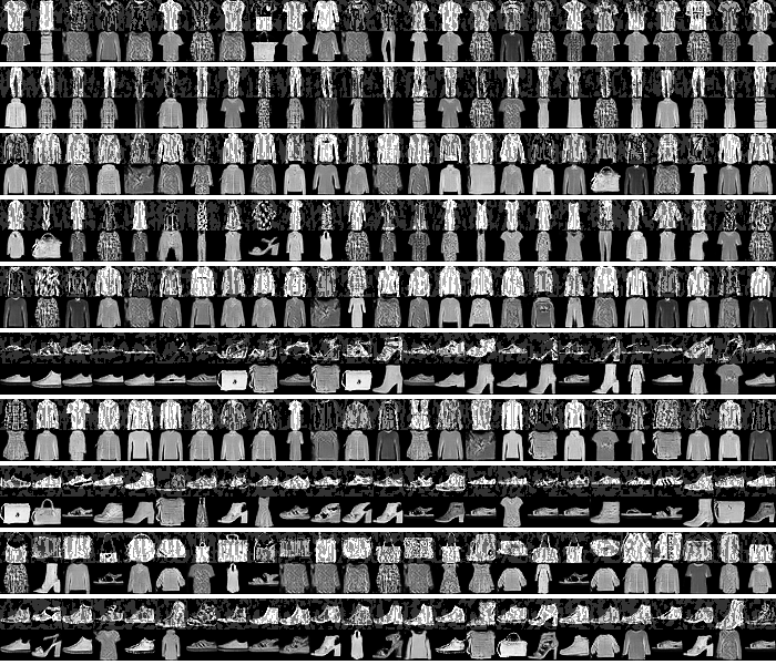
(a) FGSM

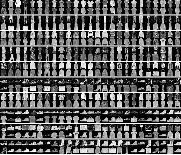
(b) BIM-a

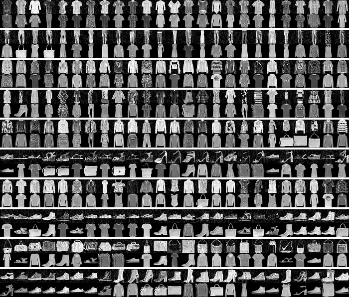
(c) BIM-b

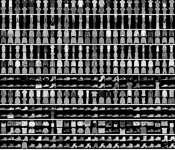
(d) CW

Figure 13: Most highly activated codewords of adversarial samples obtained with different attack strategies on FMNIST test data. Each two rows within a block show the input image (top) and corresponding codeword (bottom). Note that the adversarial images and their codeword are dissimilar in most cases.

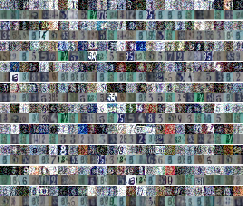
(a) FGSM

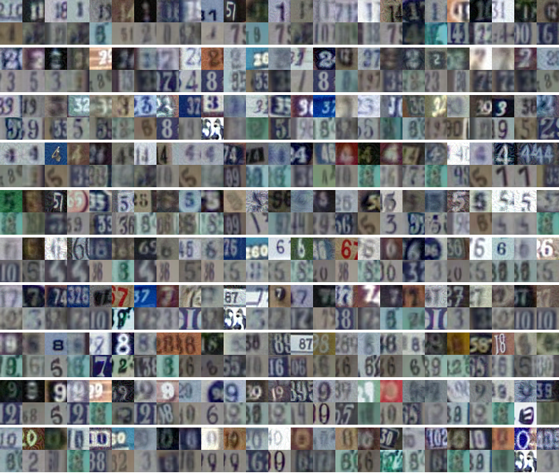
(b) BIM-a

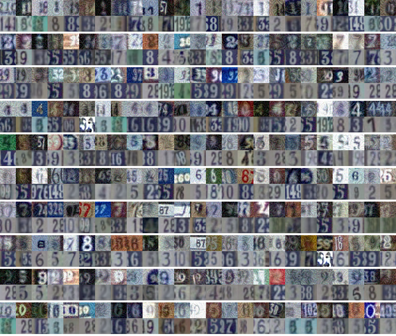
(c) BIM-b

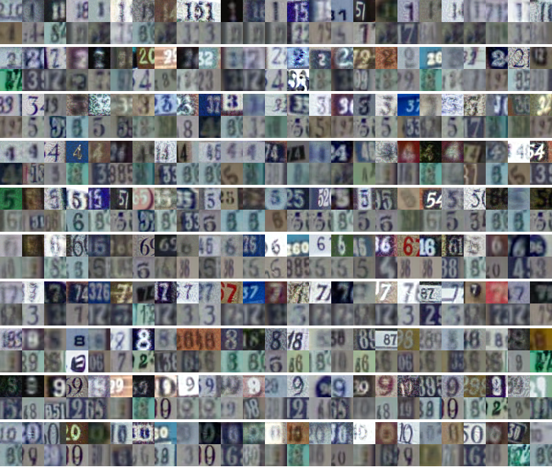
(d) CW

Figure 14: Most highly activated codewords of adversarial samples obtained with different attack strategies on SVHN test data. Each two rows within a block show the input image (top) and corresponding codeword (bottom). Note that the adversarial images and their codeword are dissimilar in most cases.

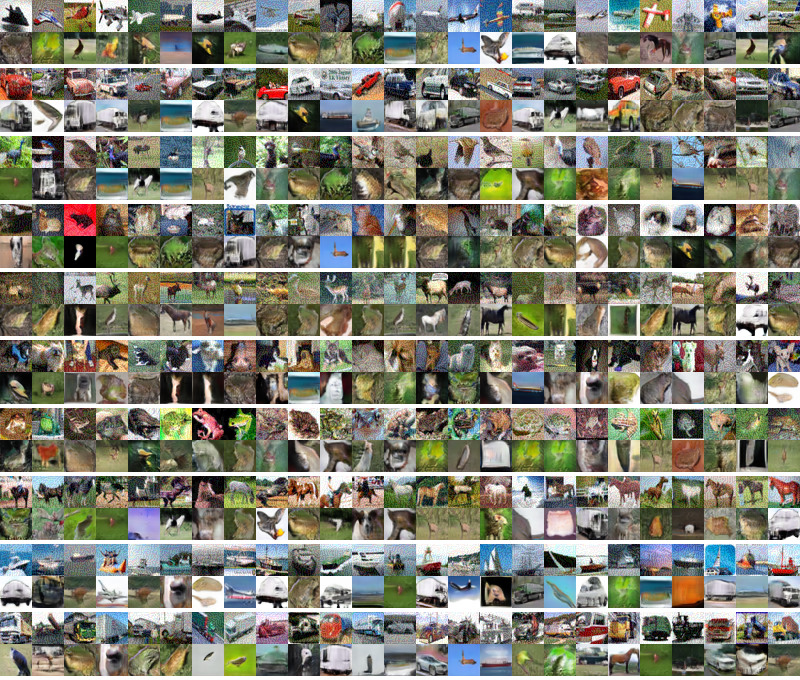
(a) FGSM

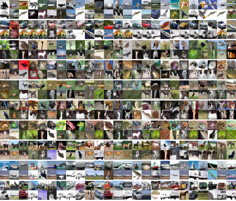
(b) BIM-a

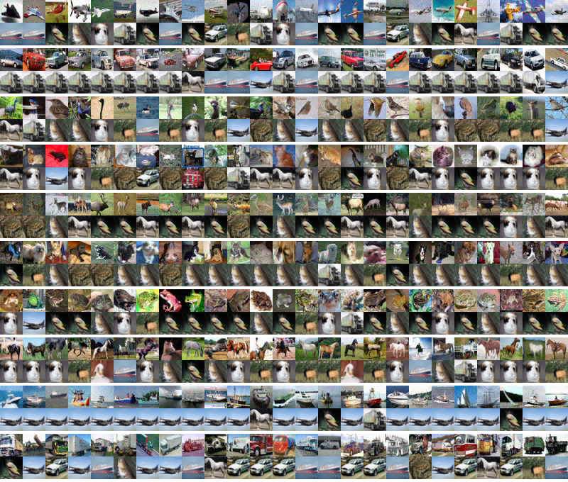
(c) BIM-b

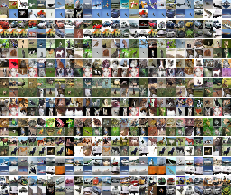
(d) CW

Figure 15: Most highly activated codewords of adversarial samples obtained with different attack strategies on CIFAR-10 test data. Each two rows within a block show the input image (top) and corresponding codeword (bottom). Note that the adversarial images and their codeword are dissimilar in most cases.

References

- [1] R. Arandjelovic, P. Gronat, A. Torii, T. Pajdla, and J. Sivic. Netvlad: Cnn architecture for weakly supervised place recognition. In Proceedings of the IEEE conference on computer vision and pattern recognition, pages 5297–5307, 2016.
- [2] R. Arandjelovic and A. Zisserman. All about vlad. In Proceedings of the IEEE conference on Computer Vision and Pattern Recognition, pages 1578–1585, 2013.
- [3] Y. Bulatov. notmnist dataset. 2011.
- [4] N. Carlini and D. Wagner. Adversarial examples are not easily detected: Bypassing ten detection methods. In Proceedings of the 10th ACM Workshop on Artificial Intelligence and Security, pages 3–14. ACM, 2017.
- [5] N. Carlini and D. Wagner. Towards evaluating the robustness of neural networks. In 2017 IEEE Symposium on Security and Privacy (SP), pages 39–57. IEEE, 2017.
- [6] R. Feinman, R. R. Curtin, S. Shintre, and A. B. Gardner. Detecting adversarial samples from artifacts. arXiv preprint arXiv:1703.00410, 2017.
- [7] P. Felzenszwalb, D. McAllester, and D. Ramanan. A discriminatively trained, multiscale, deformable part model. In Computer Vision and Pattern Recognition, 2008. CVPR 2008. IEEE Conference on, pages 1–8. IEEE, 2008.
- [8] P. F. Felzenszwalb, R. B. Girshick, D. McAllester, and D. Ramanan. Object detection with discriminatively trained part-based models. IEEE transactions on pattern analysis and machine intelligence, 32(9):1627–1645, 2010.
- [9] P. F. Felzenszwalb and D. P. Huttenlocher. Pictorial structures for object recognition. International journal of computer vision, 61(1):55–79, 2005.
- [10] R. Girdhar and D. Ramanan. Attentional pooling for action recognition. In Advances in Neural Information Processing Systems, pages 34–45, 2017.
- [11] R. Girdhar, D. Ramanan, A. Gupta, J. Sivic, and B. Russell. Actionvlad: Learning spatio-temporal aggregation for action classification. In CVPR, volume 2, page 3, 2017.
- [12] Y. Gong, L. Wang, R. Guo, and S. Lazebnik. Multi-scale orderless pooling of deep convolutional activation features. In European conference on computer vision, pages 392–407. Springer, 2014.
- [13] I. Goodfellow, J. Pouget-Abadie, M. Mirza, B. Xu, D. Warde-Farley, S. Ozair, A. Courville, and Y. Bengio. Generative adversarial nets. In Advances in neural information processing systems, pages 2672–2680, 2014.
- [14] I. J. Goodfellow, J. Shlens, and C. Szegedy. Explaining and harnessing adversarial examples (2014). arXiv preprint arXiv:1412.6572.
- [15] I. J. Goodfellow, J. Shlens, and C. Szegedy. Explaining and harnessing adversarial examples (2014). arXiv preprint arXiv:1412.6572.
- [16] K. Grosse, P. Manoharan, N. Papernot, M. Backes, and P. McDaniel. On the (statistical) detection of adversarial examples. arXiv preprint arXiv:1702.06280, 2017.
- [17] K. Grosse, P. Manoharan, N. Papernot, M. Backes, and P. McDaniel. On the (statistical) detection of adversarial examples. arXiv preprint arXiv:1702.06280, 2017.
- [18] I. Gulrajani, F. Ahmed, M. Arjovsky, V. Dumoulin, and A. C. Courville. Improved training of wasserstein gans. In Advances in Neural Information Processing Systems, pages 5767–5777, 2017.
- [19] R. Hadsell, S. Chopra, and Y. LeCun. Dimensionality reduction by learning an invariant mapping. In null, pages 1735–1742. IEEE, 2006.
- [20] K. He, X. Zhang, S. Ren, and J. Sun. Deep residual learning for image recognition. In Proceedings of the IEEE conference on computer vision and pattern recognition, pages 770–778, 2016.
- [21] D. Hendrycks and K. Gimpel. A baseline for detecting misclassified and out-of-distribution examples in neural networks. arXiv preprint arXiv:1610.02136, 2016.
- [22] H. Jegou, F. Perronnin, M. Douze, J. Sánchez, P. Perez, and C. Schmid. Aggregating local image descriptors into compact codes. IEEE transactions on pattern analysis and machine intelligence, 34(9):1704–1716, 2012.
- [23] D. P. Kingma and J. Ba. Adam: A method for stochastic optimization. arXiv preprint arXiv:1412.6980, 2014.
- [24] J. J. Koenderink and A. J. Van Doorn. The structure of locally orderless images. International Journal of Computer Vision, 31(2-3):159–168, 1999.
- [25] A. Krizhevsky and G. Hinton. Learning multiple layers of features from tiny images. Technical report, Citeseer, 2009.
- [26] A. Krizhevsky and G. Hinton. Learning multiple layers of features from tiny images. Technical report, Citeseer, 2009.
- [27] A. Krizhevsky, I. Sutskever, and G. E. Hinton. Imagenet classification with deep convolutional neural networks. In Advances in neural information processing systems, pages 1097–1105, 2012.
- [28] A. Kurakin, I. Goodfellow, and S. Bengio. Adversarial examples in the physical world. arXiv preprint arXiv:1607.02533, 2016.
- [29] B. M. Lake, R. Salakhutdinov, and J. B. Tenenbaum. Human-level concept learning through probabilistic program induction. Science, 350(6266):1332–1338, 2015.
- [30] Y. LeCun, L. Bottou, Y. Bengio, and P. Haffner. Gradient-based learning applied to document recognition. Proceedings of the IEEE, 86(11):2278–2324, 1998.
- [31] K. Lee, K. Lee, H. Lee, and J. Shin. A simple unified framework for detecting out-of-distribution samples and adversarial attacks. arXiv preprint arXiv:1807.03888, 2018.
- [32] L.-J. Li, H. Su, L. Fei-Fei, and E. P. Xing. Object bank: A high-level image representation for scene classification & semantic feature sparsification. In Advances in neural information processing systems, pages 1378–1386, 2010.
- [33] S. Liang, Y. Li, and R. Srikant. Enhancing the reliability of out-of-distribution image detection in neural networks. arXiv preprint arXiv:1706.02690, 2017.
- [34] X. Ma, B. Li, Y. Wang, S. M. Erfani, S. Wijewickrema, M. E. Houle, G. Schoenebeck, D. Song, and J. Bailey. Characterizing adversarial subspaces using local intrinsic dimensionality. arXiv preprint arXiv:1801.02613, 2018.
- [35] A. Mahendran and A. Vedaldi. Understanding deep image representations by inverting them. In Proceedings of the IEEE conference on computer vision and pattern recognition, pages 5188–5196, 2015.
- [36] A. Mahendran and A. Vedaldi. Visualizing deep convolutional neural networks using natural pre-images. International Journal of Computer Vision, 120(3):233–255, 2016.
- [37] J. H. Metzen, T. Genewein, V. Fischer, and B. Bischoff. On detecting adversarial perturbations. arXiv preprint arXiv:1702.04267, 2017.
- [38] S.-M. Moosavi-Dezfooli, A. Fawzi, and P. Frossard. Deepfool: a simple and accurate method to fool deep neural networks. In Proceedings of the IEEE Conference on Computer Vision and Pattern Recognition, pages 2574–2582, 2016.
- [39] K. K. Nakka and M. Salzmann. Deep attentional structured representation learning for visual recognition. BMVC 2018, 2018.
- [40] Y. Netzer, T. Wang, A. Coates, A. Bissacco, B. Wu, and A. Y. Ng. Reading digits in natural images with unsupervised feature learning. In NIPS workshop on deep learning and unsupervised feature learning, volume 2011, page 5, 2011.
- [41] A. Nguyen, A. Dosovitskiy, J. Yosinski, T. Brox, and J. Clune. Synthesizing the preferred inputs for neurons in neural networks via deep generator networks. In Advances in Neural Information Processing Systems, pages 3387–3395, 2016.
- [42] F. Perronnin, J. Sánchez, and T. Mensink. Improving the fisher kernel for large-scale image classification. In European conference on computer vision, pages 143–156. Springer, 2010.
- [43] P. Quelhas, F. Monay, J.-M. Odobez, D. Gatica-Perez, T. Tuytelaars, and L. Van Gool. Modeling scenes with local descriptors and latent aspects. In Computer Vision, 2005. ICCV 2005. Tenth IEEE International Conference on, volume 1, pages 883–890. IEEE, 2005.
- [44] A. Radford, L. Metz, and S. Chintala. Unsupervised representation learning with deep convolutional generative adversarial networks. arXiv preprint arXiv:1511.06434, 2015.
- [45] J. Sánchez, F. Perronnin, T. Mensink, and J. Verbeek. Image classification with the fisher vector: Theory and practice. International journal of computer vision, 105(3):222–245, 2013.
- [46] R. R. Selvaraju, M. Cogswell, A. Das, R. Vedantam, D. Parikh, D. Batra, et al. Grad-cam: Visual explanations from deep networks via gradient-based localization. In ICCV, pages 618–626, 2017.
- [47] J. Sivic and A. Zisserman. Video google: A text retrieval approach to object matching in videos. In null, page 1470. IEEE, 2003.
- [48] C. Szegedy, W. Zaremba, I. Sutskever, J. Bruna, D. Erhan, I. Goodfellow, and R. Fergus. Intriguing properties of neural networks. arXiv preprint arXiv:1312.6199, 2013.
- [49] P. Tang, X. Wang, B. Shi, X. Bai, W. Liu, and Z. Tu. Deep fishernet for object classification. arXiv preprint arXiv:1608.00182, 2016.
- [50] L. Torresani, M. Szummer, and A. Fitzgibbon. Efficient object category recognition using classemes. In European conference on computer vision, pages 776–789. Springer, 2010.
- [51] F. Wang, M. Jiang, C. Qian, S. Yang, C. Li, H. Zhang, X. Wang, and X. Tang. Residual attention network for image classification. arXiv preprint arXiv:1704.06904, 2017.
- [52] Z. Wang, H. Li, W. Ouyang, and X. Wang. Learnable histogram: Statistical context features for deep neural networks. In European Conference on Computer Vision, pages 246–262. Springer, 2016.
- [53] H. Xiao, K. Rasul, and R. Vollgraf. Fashion-mnist: a novel image dataset for benchmarking machine learning algorithms. arXiv preprint arXiv:1708.07747, 2017.
- [54] J. Xiao, J. Hays, K. A. Ehinger, A. Oliva, and A. Torralba. Sun database: Large-scale scene recognition from abbey to zoo. In Computer vision and pattern recognition (CVPR), 2010 IEEE conference on, pages 3485–3492. IEEE, 2010.
- [55] M. D. Zeiler and R. Fergus. Visualizing and understanding convolutional networks. In European conference on computer vision, pages 818–833. Springer, 2014.
- [56] Q. Zhang, Y. N. Wu, and S.-C. Zhu. Interpretable convolutional neural networks. arXiv preprint arXiv:1710.00935, 2(3):5, 2017.
- [57] B. Zhou, A. Khosla, A. Lapedriza, A. Oliva, and A. Torralba. Learning deep features for discriminative localization. In Proceedings of the IEEE Conference on Computer Vision and Pattern Recognition, pages 2921–2929, 2016.