Fast evaluation of multi-detector consistency for real-time gravitational wave searches

Abstract

Gravitational waves searches for compact binary mergers with LIGO and Virgo are presently a two stage process. First, a gravitational wave signal is identified. Then, an exhaustive search over possible signal parameters is performed. It is critical that the identification stage is efficient in order to maximize the number of gravitational wave sources that are identified. Initial identification of gravitational wave signals with LIGO and Virgo happens in real-time which requires that less than one second of computational time must be used for each one second of gravitational wave data collected. In contrast, subsequent parameter estimation may require hundreds of hours of computational time to analyze the same one second of gravitational wave data. The real-time identification requirement necessitates efficient and often approximate methods for signal analysis. We describe one piece of real-time gravitational-wave identification: an efficient method for ascertaining a signal’s consistency between multiple gravitational wave detectors suitable for real-time gravitational wave searches for compact binary mergers. This technique was used in analyses of Advanced LIGO’s second observing run and Advanced Virgo’s first observing run.

I Introduction

Advanced LIGO Harry et al. (2010); Aasi et al. (2015) and Virgo Acernese et al. (2014) gravitational-wave observatories have seen great success since the discovery of gravitational waves in September 2015 Abbott et al. (2016a). With the detection of gravitational waves from ten binary black holes and one binary neutron star in just 170 days of observing, gravitational wave detections are now happening at a rate of about two per month of multi-detector observation time Abbott et al. (2018a). The rate is expected to increase by more than an order of magnitude as the world-wide network of gravitational wave detectors improve in sensitivity Abbott et al. (2018b). Furthermore, over the next decade, the gravitational wave detector network will grow to include KAGRA Somiya (2012); Aso et al. (2013) in Japan and LIGO-India Unnikrishnan (2013). It is anticipated that real-time gravitational wave searches will use data from the entire gravitational wave detector network in order to increase the detection rate and better localize the gravitational wave sources Abbott et al. (2018b).

The current generation of interferometric gravitational wave detectors measure only one of two possible gravitational wave polarizations $h_{+}$ and $h_{\times}$. However, given the detector orientation with respect to incoming signals, they each measure a different linear combination of polarizations defined by a suitable Earth-centered coordinate system. Furthermore, the response to the gravitational wave signal changes as a function of the incident angle. While the detector response function is broad, some incident angles produce no response in a given gravitational wave detector. Thus, each detector’s response to a given signal is a function of the location and polarization state of a gravitational wave source Abbott et al. (2009); Harry et al. (2010); Acernese et al. (2014). Given a particular gravitational wave signal incident on Earth, it is possible to predict precisely what the projection of the signal will be on each of the gravitational wave detectors Anderson et al. . A corollary of this is that only certain arrival times, phases and amplitudes measured in a set of gravitational wave detectors are consistent with a real gravitational wave signal.

Typically, gravitational wave searches have relied on one of several mechanisms for imposing consistency of gravitational wave detection among a network of detectors. Each method has a varying degree of fidelity traded against complexity or computational cost. The ideal method requires explicitly evaluating the likelihood of measuring the projected waveform in each detector while sampling over physically reasonable prior distributions, e.g., isotropically distributed on the sky, using Markov Chain Monte Carlo techniques Veitch et al. (2015). This is the method used in parameter estimation as the second stage of gravitational wave astronomy. While regarded as the most accurate assessment of consistency among gravitational wave detectors, the full likelihood evaluation has the practical limitation of being a computationally costly procedure. However, approximate methods have been developed Singer and Price (2016), that are used to e.g., quickly compute the sky location of gravitational wave events. The approximate methods are orders of magnitude faster and still extremely accurate. Nevertheless, the approximate methods used to compute sky maps are not suitably fast to use for the initial identification stage of gravitational wave events.

Another widely adopted mechanism to ensure consistency between gravitational wave observatories is to form a coherent combination of the detector data Pai et al. (2002); Macleod et al. (2016) in order to create a sky location dependent reconstruction of the two gravitational wave polarizations. This technique typically uses a predefined grid of sky positions. Coherence is used presently in searches for gravitational wave bursts Klimenko et al. (2008); Sutton et al. (2010) and triggered searches for gamma ray bursts Harry and Fairhurst (2011); Williamson et al. (2014) which only focus on specific time intervals and sky regions that overlap with known gamma ray bursts.

The final mechanism involves searching each detector data stream independently, triggering on potential signal times by finding peaks in filter output over some time interval, and then comparing the triggers between each detector to see if they are consistent with a signal Babak et al. (2013); Usman et al. (2016); Messick et al. (2017). The simplest implementations of this procedure impose that triggers occur within the gravitational wave propagation time between detectors, but don’t otherwise place constraints on the amplitude or phase measured in each detector. However, not all gravitational-wave arrival times are probable or even possible when considering a network of gravitational wave detectors. Furthermore, arrival times are strongly correlated with the measured amplitude and phase of the gravitational wave signals. Ignoring these effects means that one increases the background (false-positive rate) of a given gravitational-wave search by considering unphysical gravitational wave signals.

Work to check consistency of the distribution of measured amplitude, time and phase of gravitational wave triggers from a network of detectors has been explored in several contexts. The early work used only one-dimensional marginalized distributions for these parameters Cannon (2008), which did not accurately describe the joint probability for the network but was nevertheless demonstrably more effective than simply using coarse windows in arrival time to define coincidences. A joint probability distribution of signal amplitudes for the LIGO and Virgo network was developed for compact binary searches in  Cannon et al. (2015) and used during advanced LIGO’s first observing run, however time of arrival and phase parameters were ignored. Explicitly constructing probabilities for time, phase and amplitude for the two LIGO detectors and using this information in ranking of candidate events was explored in the second Advanced LIGO observing run Nitz et al. (2017).

In this work, we present a method for accounting for signal consistency in compact binary searches across a network of gravitational wave detectors that is computationally efficient and will scale to the eventual 5 detector gravitational wave network. This is accomplished through a factorization of the likelihood ratio (LR) ranking statistic first described in  Cannon et al. (2015) and used in the analysis of candidates from the compact binary coalescence search in the first observing run O1 Messick et al. (2017); Sachdev et al. ; Abbott et al. (2016b, c, d, a) that generalizes to multiple gravitational wave detectors, and which takes into account the correlated trigger amplitudes, times and phases between multiple gravitational wave observatories. While the main objective of this work is to document a novel gravitational wave detection algorithm, it also serves as a reference for methods used in LIGO and Virgo searches in Advanced LIGO’s second observing run and advanced Virgo’s first observing run Abbott et al. (2018a).

II The Likelihood Ratio

In this section we describe the likelihood ratio (LR) ranking statistic as implemented in the GstLAL inspiral pipeline Messick et al. (2017); Sachdev et al. ; LIGO Scientific Collaboration and Virgo Collaboration (2018a) with an emphasis on terms relevant to this particular discussion. In brief, the GstLAL inspiral pipeline analyzes data from multiple gravitational wave detectors with time-domain matched filtering Cannon et al. (2012) over a collection of gravitational wave templates. First, the peaks in each template filter output are identified for each detector. Then, these peaks, which are called triggers, are combined to look for coincident triggers in the gravitational wave network. If triggers from the same template are within the gravitational wave propagation time between observatories, the collection of triggers is called a coincident event Privitera et al. (2014).

Coincident events are common and the vast majority are not gravitational waves. This is due to the fact that the threshold in each detector for identifying a trigger is very low leading to potentially billions of triggers per analysis and tens of millions found in coincidence. Therefore, we have to rank the collection of coincident events from least to most probable of being a gravitational wave. To do this, we explicitly evaluate the LR over the trigger parameters. We consider a LR ranking statistic for gravitational-wave candidates defined as 

$$\mathcal{L} =\frac{P(\,\vec{D_{H}},\vec{O},\vec{\rho},\vec{\xi^{2}},\vec{\phi},\vec{t}\mid\mathrm{s}\,)}{P(\,\vec{D_{H}},\vec{O},\vec{\rho},\vec{\xi^{2}},\vec{\phi},\vec{t}\mid\mathrm{n}\,)}.$$ (1)

Each vector of parameters is used to denote detector specific information. To be concrete we will assume that LIGO Hanford, $H1$, LIGO Livingston, $L1$, and Virgo, $V1$ are all in observing mode and being analyzed. However, we note that the method described can be generalized to add more detectors. $\vec{D_{H}}$ is a vector of horizon distances for each observatory $\vec{D_{H}}=\{D_{\mathrm{H1}},D_{\mathrm{L1}},D_{\mathrm{V1}}\}$, which accounts for how sensitive the detectors are at the time of the event. $\vec{O}$ is the set of detectors that observed the event in coincidence. Since it is possible for a gravitational wave to not register in one or more detectors above threshold, $\vec{O}$ will take on one of six possible values in this case: $\vec{O}\in\{\{H1,L1,V1\}$ , $\{H1,L1\}$, $\{H1,V1\}$, $\{L1,V1\}$, $\{H1\}$, $\{L1\}$, $\{V1\}\}$. $\vec{\rho}$ is the vector individual signal-to-noise ratios (SNRs) in each detector, e.g., $\vec{\rho}=\{\rho_{\mathrm{H1}},\rho_{\mathrm{L1}},\rho_{\mathrm{V1}}\}$ and $\vec{\xi^{2}}$ is the vector of $\xi^{2}$-signal-based-veto values for each detector (described in Messick et al. (2017)), e.g., $\vec{\xi^{2}}=\{\xi^{2}_{\mathrm{H1}},\xi^{2}_{\mathrm{L1}},\xi^{2}_{\mathrm{V1}}\}$. Likewise, $\vec{t}$ and $\vec{\phi}$ are the time and phases measured at each gravitational wave detector Allen et al. (2012), $\vec{t}=\{t_{\mathrm{H1}},t_{\mathrm{L1}},t_{\mathrm{V1}}\}$ and $\vec{\phi}=\{\phi_{\mathrm{H1}},\phi_{\mathrm{L1}},\phi_{\mathrm{V1}}\}$.

The independence between detectors for noise events implies that the denominator of (1), $P(\,\ldots\mid\mathrm{n}\,)$, factors to the product of one-dimensional and two-dimensional distributions and is therefore generally easy to estimate and evaluate numerically. The numerator, $P(\,\ldots\mid\mathrm{s}\,)$ is not easily factorable. Reference Cannon et al. (2015) outlines the factorization of Eq. 1 without the $\vec{\Delta\phi}$ and $\vec{\Delta t}$ terms, though we point out that it does include the joint distribution of SNR. This form was used in the ranking of gravitational-wave candidates from the first observing run, O1, during which only the H1 and L1 advanced LIGO detectors were operating Abbott et al. (2016a, c). Here we extend the technique used in Cannon et al. (2015) and propose the following factorization of the numerator,

$$P(\,\ldots\mid\mathrm{s}\,) =P(\,\vec{D_{H}}\mid\mathrm{s}\,)$$

$$\times P(\,\vec{O}\mid\vec{D_{H}},\mathrm{s}\,)$$

$$\times P(\,\vec{\xi^{2}}\mid\vec{\rho},\mathrm{s}\,)$$

$$\times P(\,\vec{\rho},\vec{\phi},\vec{t}\mid\vec{O},\vec{D_{H}},\mathrm{s}\,),$$ (2)

where we assume that the distribution of the $\vec{\xi^{2}}$-signal-based-veto values are independent of $\vec{\phi}$ and $\vec{t}$ but not $\vec{\rho}$.

In this work we are concerned with an approximation to the final term: $P(\,\vec{\rho},\vec{\phi},\vec{t}\mid\vec{O},\vec{D_{H}},\mathrm{s}\,)$, which accounts for the amplitude, time, and phase measured in each gravitational wave detector. We begin by isolating an overall term that scales with the detector network SNR, $\left|\,\vec{\rho}\,\right|$, to the negative fourth power Schutz (2011) so that

$$P(\,\vec{\rho},\vec{\phi},\vec{t}\mid\vec{O},\vec{D_{H}},\mathrm{s}\,)\approx\\ P(\,\vec{\rho}/\left|\,\vec{\rho}\,\right|,\vec{\phi},\vec{t}\mid\vec{O},\vec{D_{H}},\mathrm{s}\,)\times\left|\,\vec{\rho}\,\right|^{-4}$$ (3)

This approximation ignores the fact that the accuracy of the measured $\vec{\phi}$ and $\vec{t}$ depend on the SNR, $\vec{\rho}$. In other words, at low SNR the distribution of time and phase is broad and at high SNR it is narrow. However, since it is most critical for the detection process to catch signals that are near threshold, we assume that the uncertainty in $\vec{t}$ and $\vec{\phi}$ take on values consistent with a network SNR $\sim 10$. Thus, our goal is to adequately describe the $P(\,\vec{\rho}/\left|\,\vec{\rho}\,\right|,\vec{\phi},\vec{t}\mid\vec{O},\vec{D_{H}},\mathrm{s}\,)$ when the network SNR is about 10.

Next, we note that the absolute time and phase of the signal is arbitrary. Assuming isotropically distributed gravitational waves, the distribution of time and phase at a given detector is uniform. However, the relative times and phases between detectors make up a nontrivial correlated probability density function. This suggests that we can reduce the dimensionality by computing parameters relative to a fiducial instrument either by difference or ratio. We pick the first instrument in alphabetical order. Furthermore, since $P(\,\vec{\rho}/\left|\,\vec{\rho}\,\right|,\vec{\phi},\vec{t}\mid\vec{O},\vec{D_{H}},\mathrm{s}\,)$ is conditional on the detector horizon distances, we can evaluate the effective distances, $\vec{D_{\text{eff}}}=\{d_{\mathrm{H1}},d_{\mathrm{L1}},d_{\mathrm{V1}}\}$ Allen et al. (2012) instead of $\vec{\rho}$. The advantage to switching to effective distances, is that the distribution of effective distance ratios is constant. Thus we have,

$$P(\,\vec{\rho},\vec{\phi},\vec{t}\mid\vec{O},\vec{D_{H}},\mathrm{s}\,)\overset{\propto}{\sim}\\ P(\,\vec{\Delta\ln D_{\text{eff}}},\vec{\Delta\phi},\vec{\Delta t}\mid\vec{O},\mathrm{s}\,)\times\left|\,\vec{\rho}\,\right|^{-4},$$ (4)

where concretely for the $H1$, $L1$, $V1$ network

$$\vec{\Delta\ln D_{\text{eff}}} \equiv\{\ln(d_{L1}/d_{H1}),\ln(d_{V1}/d_{H1})\},$$

$$\vec{\Delta t} \equiv\{t_{L1}-t_{H1},t_{V1}-t_{H1}\},$$

$$\vec{\Delta\phi} \equiv\{\phi_{L1}-\phi_{H1},\phi_{V1}-\phi_{H1}\}.$$

In interest of simplifying the subsequent notation, we define a single vector of parameters that contains $\vec{\Delta\ln D_{\text{eff}}}$, $\vec{\Delta t}$ and $\vec{\Delta\phi}$,

$$\vec{\lambda} \equiv\{\vec{\Delta\ln D_{\text{eff}}},\vec{\Delta t},\vec{\Delta\phi}\}.$$ (5)

In order to construct the distribution of these parameters for a signal, we assert that gravitational waves have a uniform distribution in Earth-based coordinates: right ascension $\alpha$, declination $\cos(\delta)$, inclination angle $\cos(\iota)$, and polarization angle $\psi$. We lay down a uniform, densely sampled grid in $\{\alpha,\cos(\delta),\cos(\iota),\psi\}$ and further assert that any signal should “exactly” land on one of the grid points. We transform that regularly-spaced grid into a grid of irregularly spaced points in $\vec{\lambda}$, which we denote as $\vec{\lambda}_{\mathrm{mi}}$ for the $i^{th}$ model vector. We consider that the only mechanism to push a signal away from one of these exact $i^{th}$ grid points is Gaussian noise. Furthermore we assume the probability distribution is of the form:

$$P(\,\vec{\lambda}\mid\vec{O},\mathrm{s},\vec{\lambda}_{\mathrm{mi}}\,)=\\ \frac{1}{\sqrt{(2\pi)^{k}|\boldsymbol{\Sigma}_{\vec{\lambda}}|}}\exp{\left[-\frac{1}{2}\vec{\Delta\lambda}_{i}\boldsymbol{\Sigma}^{-1}_{\vec{\lambda}}\vec{\Delta\lambda}_{i}^{T}\right]},$$ (6)

where $\vec{\Delta\lambda}_{i}\equiv\vec{\lambda}-\vec{\lambda}_{\mathrm{mi}}$ and $\boldsymbol{\Sigma}_{\vec{\lambda}}$ is a covariance matrix of $\vec{\lambda}$. We further assume that the measurement of the time, phase, effective distance for an individual detector is independent of that for the other detectors. Therefore, every element of $\vec{\lambda}$ can be expressed as

$$\Sigma_{ij}={\sigma^{2}}_{\lambda_{i}\lambda_{j}}={\sigma^{2}}_{\theta_{i}\theta_{j}}^{(\mathrm{ifo}1)}+{\sigma^{2}}_{\theta_{i}\theta_{j}}^{(\mathrm{ifo}2)},$$ (7)

where $\vec{\theta}$ is a vector of the three extrinsic parameters of interest, namely $\vec{\theta}\equiv\{\ln D_{\textrm{eff}},t,\phi\}$, and the superscripts (ifo1/2) indicate an individual detector in a pair, at which the parameters are measured. The covariance matrix on $\vec{\theta}$ can be approximated by the inverse of a Fisher information matrix. Hence, one can obtain the covariance matrix as follows:

$$\boldsymbol{\Sigma}_{\vec{\theta}} \equiv\begin{bmatrix}{\sigma^{2}}_{tt}&{\sigma^{2}}_{t\phi}&{\sigma}^{2}_{t\ln D_{\textrm{eff}}}\\ {\sigma^{2}}_{\phi t}&{\sigma^{2}}_{\phi\phi}&{\sigma^{2}}_{\phi\ln D_{\textrm{eff}}}\\ {\sigma^{2}}_{\ln D_{\textrm{eff}}\,t}&{\sigma^{2}}_{\ln D_{\textrm{eff}}\,\phi}&{\sigma^{2}}_{\ln D_{\textrm{eff}}\ln D_{\textrm{eff}}}\end{bmatrix}$$ (8)

$$=\begin{bmatrix}\frac{1}{\big{(}2\pi\,\rho\,\sigma_{f}\big{)}^{2}}&\frac{\mathrm{bar}{f}}{2\pi\,\rho^{2}\,\sigma_{f}^{2}}&0\\ \frac{\mathrm{bar}{f}}{2\pi\,\rho^{2}\,\sigma_{f}^{2}}&\frac{\mathrm{bar}{f^{2}}}{\big{(}\rho\,\sigma_{f}\big{)}^{2}}&0\\ 0&0&\frac{1}{\rho^{2}}\end{bmatrix}.$$ (9)

$\sigma_{f}$ is the effective bandwidth of the signal, defined as Fairhurst (2009)

$$\sigma_{f}^{2}\equiv\mathrm{bar}{f^{2}}-\left(\mathrm{bar}{f^{1}}\right)^{2},$$ (10)

using the frequency moments of the signal

$$\mathrm{bar}{f^{n}}\equiv 4\int_{0}^{\infty}df\frac{|\tilde{h}(f)|^{2}}{S(f)}f^{n}.$$ (11)

From Eq. 8, it is clear that the covariance matrix elements depend on the observed SNR at each detector. Since the goal of the present work is to improve efficiency of detecting near threshold triggers, we have set the characteristic SNR for Hanford, Livingston and Virgo detector as 5, 7 and 2.25 respectively.

The inverse of the covariance matrix $\boldsymbol{\Sigma}_{\vec{\lambda}}$ further can be decomposed into following two matrices using Cholesky decomposition Golub and Van Loan (2012).

$$\big{(}\boldsymbol{\Sigma}_{\vec{\lambda}}\big{)}^{-1}=\bf{\mathcal{C}}\,\bf{\mathcal{C}}^{T},$$ (12)

where $\bf{\mathcal{C}}$ is a lower triangular matrix. The matrix $\bf{\mathcal{C}}$ is then used to obtain a re-scaled set of orthogonal coordinates $\vec{x}$ such that $\vec{\Delta x}_{i}\equiv\Big{(}\vec{\lambda}-\vec{\lambda}_{\mathrm{mi}}\Big{)}\,\mathcal{C}=\Delta\vec{\lambda}_{i}\,\mathcal{C}$. Hence, the probability distribution described in the Eq.(6) can be rewritten in terms of the new coordinates as

$$P\Big{(}\vec{\lambda}|\vec{O},s,\vec{\lambda}_{\textrm{mi}}\Big{)}\propto\textrm{exp}\Big{[}-\frac{1}{2}\vec{\Delta x_{i}}^{2}\Big{]}$$ (13)

Then we assert that

$$P(\,\vec{\lambda}\mid\vec{O},\mathrm{s}\,) \propto\sum_{i}P(\,\vec{\lambda}\mid\vec{O},\mathrm{s},\vec{\lambda}_{\mathrm{mi}}\,)P\left(\vec{\lambda}_{\mathrm{mi}}\right)$$

$$\propto\sum_{i}P(\,\vec{\lambda}\mid\vec{O},\mathrm{s},\vec{\lambda}_{\mathrm{mi}}\,)$$

$$=\sum_{i}\exp{\left[-\frac{1}{2}\vec{\Delta x}_{i}^{2}\right]},$$ (14)

where the second line holds by construction since $P\left(\vec{\lambda}_{\mathrm{mi}}\right)$ does not depend on $i$ as they were chosen uniform in prior signal probability. Computing probability (II) in real-time for each gravitational wave candidate is not feasible since the grid might have millions of points. Therefore, we make another simplifying assumption: we assume that the noise only adds a contribution which is orthogonal to the hyper-surface defined by the signal. In other words, we assume that noise cannot push a signal from one grid point towards another along the signal hyper-surface which implies,

$$\vec{\Delta x}_{i}^{2}\approx\vec{\Delta x}_{0}^{2}+g_{0i}^{2},$$ (15)

where $\vec{\Delta x}_{0}$ refers to the distance between the candidate parameter and the nearest-neighbor grid point, and $g_{0i}$ is the distance between the $i$th grid point and the nearest neighbor grid point. In this case we can simplify the marginalization step with a precomputation since

$$P(\,\vec{\lambda}\mid\vec{O},\mathrm{s}\,) \approx\exp{\left[-\frac{1}{2}\vec{\Delta x}_{0}^{2}\right]}$$

$$\times\sum_{i}\exp{\left[-\frac{1}{2}g_{0i}^{2}\right]}.$$ (16)

The entire sum over $i$ can be precomputed and stored. In order for this endeavor to be successful, we still need a fast way to find the nearest neighbor. We use SciPy KDTree to accomplish this Jones et al. (2014). Fig. 1 shows an example probability density function for time delays and phase differences between LIGO Hanford and Virgo computed from the above method as well as a comparison with $1\times 10^{5}$ samples produced by a direct Monte Carlo. Fig. 2 is a probability-probability (p-p) plot created by a subset of the samples shown in Fig. 1. We find that the drawn samples are in a good agreement with the two dimensional distribution over phase and time. We note that each evaluation of (II) required less than a millisecond to compute on a modern CPU. Thus, this method is suitable for evaluating hundreds of candidates per second per CPU core in real-time.

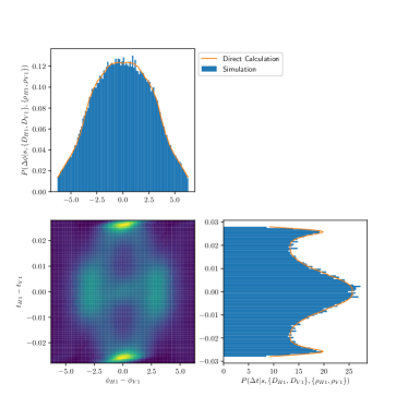
Figure 1: Example probability density function for the difference in gravitational wave arrival time and phase between LIGO Hanford and Virgo. Here we set the horizon distances of LIGO Hanford and Virgo to be $110~{}\mathrm{Mpc}$ and $45~{}\mathrm{Mpc}$ respectively to be consistent with realistic PSDs of the two detectors, which are used for (11), and show a slice of the probability density function where the ratios of the effective distance are close to 1. The full two dimensional distribution (lower left) was computed using the method described in section II. The orange traces use the data from the two dimensional distribution marginalized over phase and time respectively. For comparison, we computed the marginal distributions via a direct Monte Carlo method to obtain the top and bottom right bar plots. The agreement is excellent, however, we note that the same error assumptions were used in the Monte Carlo method and that changing the assumptions about the covariance matrix will lead to poorer agreement.

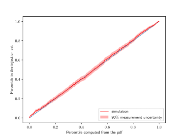
Figure 2: P-p plot created by a subset of the Monte Carlo samples shown in Fig. 1. The uncertainty on the measured percentiles due to a finite number of samples is shown as shaded region. We find that the diagonal line sits in the error region in the entire percentile random which indicates an agreement between the samples and the two dimensional distribution.

III Results

To assess the effect of the procedure described in II, we conducted a simulation of synthetic signals and non-stationary noise in order to produce a Receiver Operating Characteristics (ROC) curve. We constructed synthetic signal and noise models. For the signal model, we assumed sources uniform in the volume of space and isotropically oriented. We constructed $1\times 10^{7}$ such signals and calculated their corresponding SNRs, arrival times, and phases in the LIGO Hanford and LIGO Livingston detectors using the LAL Simulation package LIGO Scientific Collaboration and Virgo Collaboration (2018b). For noise, we constructed $1\times 10^{7}$ simulated glitches with SNRs that were independent in each of the LIGO Hanford and LIGO Livingston detectors given by an exponential distribution

$$P\left(\rho_{H1},\rho_{L1}\right)=\frac{1}{6}\exp(-\frac{\rho_{H1}}{6})\,\frac{1}{6}\exp(-\frac{\rho_{L1}}{6}),$$ (17)

where we placed an additional constraint that we only kept samples which had both $\rho_{H1}\geq 4$ and $\rho_{L1}\geq 4$. We chose arrival time differences that were uniform within the GW travel time between the two detectors and phase differences that were uniform between 0 and $2\pi$.

Figure 3 shows the ROC curves for three cases: the SNR-only terms in the LR, which was used in initial advanced LIGO searches Abbott et al. (2016a, c, b) (green); a previous implementation of time and phase consistency used for subsequent gravitational wave searches Sachdev et al. ; Scientific et al. (2017); Abbott et al. (2017a); abb (2017); Abbott et al. (2017b) terms (orange); and finally the current implementation described in section II (blue). Here we see that even in the two-detector situation, the current implementation achieves an improvement for the false alarm probability above $1\times 10^{-3}$.

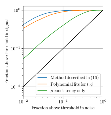
Figure 3: ROC curve showing performance of signal consistency check from the simulation described in III. The ROC curve plots the fraction of simulated events found above a given threshold of LR vs the fraction of noise found above that threshold. The black diagonal line would indicate that the method is not helpful at discriminating signals from noise. It is desirable to have the performance of any method be above the black diagonal line. The green curve shows the likelihood ratio including only the amplitude consistency terms ($\vec{\rho}$) used in the first advanced LIGO observing run Cannon et al. (2015). The orange curve shows the inclusion of $\vec{\Delta t}$ and $\vec{\Delta\phi}$ terms used in the beginning of advanced LIGO’s second observing run Sachdev et al. and the blue curve shows method described in section II.

IV Conclusion

We have demonstrated a computationally efficient likelihood ratio statistic for use in gravitational wave searches for compact binary systems with LIGO and Virgo. The work here specifically presents a way to assess the probability that a given set of measurements independently made at each observatory in a worldwide network of observatories is consistent with a signal. This is useful for real-time identification of candidates where the latency of the computation is critical and the overall computational scale cannot be too large. Our method allows for computing the likelihood ratio for hundreds of candidates per second on a single modern CPU core. This method was used to produce the final results for advanced LIGO’s second observing run and Advanced Virgo’s first observing run with the GstLAL pipeline.

V Acknowledgements

This work was supported by the National Science Foundation through PHY-1454389, OAC-1841480, ACI-1642391, PHY-1700765, and PHY-1607585. Funding for this project was provided by the Charles E. Kaufman Foundation of The Pittsburgh Foundation. We thank the LIGO Scientific Collaboration for input on this work. Specifically, CH would like to thank Patrick Brady for several illuminating discussions. This research was supported in part by Perimeter Institute for Theoretical Physics. Research at Perimeter Institute is supported by the Government of Canada through the Department of Innovation, Science, and Economic Development, and by the Province of Ontario through the Ministry of Research and Innovation. Computations for this research were performed on the Pennsylvania State University’s Institute for CyberScience Advanced CyberInfrastructure (ICS-ACI). We are grateful for computational resources provided by the Leonard E Parker Center for Gravitation, Cosmology and Astrophysics at the University of Wisconsin-Milwaukee and supported by National Science Foundation Grants PHY-1626190 and PHY-1700765. The authors are grateful for computational resources provided by the LIGO Laboratory and supported by National Science Foundation Grants PHY-0757058 and PHY-0823459. This paper has LIGO document number: P1800362.

References

- Harry et al. (2010) G. M. Harry, L. S. Collaboration, et al., Classical and Quantum Gravity 27, 084006 (2010).
- Aasi et al. (2015) J. Aasi, B. Abbott, R. Abbott, T. Abbott, M. Abernathy, K. Ackley, C. Adams, T. Adams, P. Addesso, R. Adhikari, et al., Classical and quantum gravity 32, 074001 (2015).
- Acernese et al. (2014) F. Acernese, M. Agathos, K. Agatsuma, D. Aisa, N. Allemandou, A. Allocca, J. Amarni, P. Astone, G. Balestri, G. Ballardin, et al., Classical and Quantum Gravity 32, 024001 (2014).
- Abbott et al. (2016a) B. P. Abbott, R. Abbott, T. Abbott, M. Abernathy, F. Acernese, K. Ackley, C. Adams, T. Adams, P. Addesso, R. Adhikari, et al., Physical review letters 116, 061102 (2016a).
- Abbott et al. (2018a) B. P. Abbott et al., arXiv preprint arXiv:1811.12907 (2018a).
- Abbott et al. (2018b) B. Abbott, R. Abbott, T. Abbott, et al., Living Reviews in Relativity 21 (2018b).
- Somiya (2012) K. Somiya, Classical and Quantum Gravity 29, 124007 (2012).
- Aso et al. (2013) Y. Aso, Y. Michimura, K. Somiya, M. Ando, O. Miyakawa, T. Sekiguchi, D. Tatsumi, H. Yamamoto, K. Collaboration, et al., Physical Review D 88, 043007 (2013).
- Unnikrishnan (2013) C. Unnikrishnan, International Journal of Modern Physics D 22, 1341010 (2013).
- Abbott et al. (2009) B. Abbott, R. Abbott, R. Adhikari, P. Ajith, B. Allen, G. Allen, R. Amin, S. Anderson, W. Anderson, M. Arain, et al., Reports on Progress in Physics 72, 076901 (2009).
- (11) W. G. Anderson, J. T. Whelan, P. R. Brady, J. D. Creighton, D. Chin, and K. Riles, .
- Veitch et al. (2015) J. Veitch, V. Raymond, B. Farr, W. Farr, P. Graff, S. Vitale, B. Aylott, K. Blackburn, N. Christensen, M. Coughlin, et al., Physical Review D 91, 042003 (2015).
- Singer and Price (2016) L. P. Singer and L. R. Price, Physical Review D 93, 024013 (2016).
- Pai et al. (2002) A. Pai, S. Bose, and S. Dhurandhar, Classical and Quantum Gravity 19, 1477 (2002).
- Macleod et al. (2016) D. Macleod, I. Harry, and S. Fairhurst, Physical Review D 93, 064004 (2016).
- Klimenko et al. (2008) S. Klimenko, I. Yakushin, A. Mercer, and G. Mitselmakher, Classical and Quantum Gravity 25, 114029 (2008).
- Sutton et al. (2010) P. J. Sutton, G. Jones, S. Chatterji, P. Kalmus, I. Leonor, S. Poprocki, J. Rollins, A. Searle, L. Stein, M. Tinto, et al., New Journal of Physics 12, 053034 (2010).
- Harry and Fairhurst (2011) I. W. Harry and S. Fairhurst, Physical Review D 83, 084002 (2011).
- Williamson et al. (2014) A. R. Williamson, C. Biwer, S. Fairhurst, I. Harry, E. Macdonald, D. Macleod, and V. Predoi, Physical Review D 90, 122004 (2014).
- Babak et al. (2013) S. Babak, R. Biswas, P. Brady, D. A. Brown, K. Cannon, C. D. Capano, J. H. Clayton, T. Cokelaer, J. D. Creighton, T. Dent, et al., Physical Review D 87, 024033 (2013).
- Usman et al. (2016) S. A. Usman, A. H. Nitz, I. W. Harry, C. M. Biwer, D. A. Brown, M. Cabero, C. D. Capano, T. Dal Canton, T. Dent, S. Fairhurst, et al., Classical and Quantum Gravity 33, 215004 (2016).
- Messick et al. (2017) C. Messick, K. Blackburn, P. Brady, P. Brockill, K. Cannon, R. Cariou, S. Caudill, S. J. Chamberlin, J. D. Creighton, R. Everett, et al., Physical Review D 95, 042001 (2017).
- Cannon (2008) K. C. Cannon, Classical and Quantum Gravity 25, 105024 (2008).
- Cannon et al. (2015) K. Cannon, C. Hanna, and J. Peoples, ArXiv e-prints (2015), arXiv:1504.04632 [astro-ph.IM] .
- Nitz et al. (2017) A. H. Nitz, T. Dent, T. Dal Canton, S. Fairhurst, and D. A. Brown, The Astrophysical Journal 849, 118 (2017).
- (26) S. Sachdev et al., in prep. .
- Abbott et al. (2016b) B. Abbott, R. Abbott, T. Abbott, M. Abernathy, F. Acernese, K. Ackley, C. Adams, T. Adams, P. Addesso, R. Adhikari, et al., Physical Review X 6, 041015 (2016b).
- Abbott et al. (2016c) B. P. Abbott, R. Abbott, T. Abbott, M. Abernathy, F. Acernese, K. Ackley, C. Adams, T. Adams, P. Addesso, R. Adhikari, et al., Physical review letters 116, 241103 (2016c).
- Abbott et al. (2016d) B. P. Abbott, R. Abbott, T. Abbott, M. Abernathy, F. Acernese, K. Ackley, C. Adams, T. Adams, P. Addesso, R. Adhikari, et al., Physical Review D 93, 122003 (2016d).
- LIGO Scientific Collaboration and Virgo Collaboration (2018a) LIGO Scientific Collaboration and Virgo Collaboration, “Gstlal,” (2018a).
- Cannon et al. (2012) K. Cannon, R. Cariou, A. Chapman, M. Crispin-Ortuzar, N. Fotopoulos, M. Frei, C. Hanna, E. Kara, D. Keppel, L. Liao, et al., The Astrophysical Journal 748, 136 (2012).
- Privitera et al. (2014) S. Privitera, S. R. Mohapatra, P. Ajith, K. Cannon, N. Fotopoulos, M. A. Frei, C. Hanna, A. J. Weinstein, and J. T. Whelan, Physical Review D 89, 024003 (2014).
- Allen et al. (2012) B. Allen, W. G. Anderson, P. R. Brady, D. A. Brown, and J. D. Creighton, Physical Review D 85, 122006 (2012).
- Schutz (2011) B. F. Schutz, Classical and Quantum Gravity 28, 125023 (2011).
- Fairhurst (2009) S. Fairhurst, New Journal of Physics 11, 123006 (2009).
- Golub and Van Loan (2012) G. H. Golub and C. F. Van Loan, Matrix computations, Vol. 3 (JHU press, 2012).
- Jones et al. (2014) E. Jones, T. Oliphant, and P. Peterson, (2014).
- LIGO Scientific Collaboration and Virgo Collaboration (2018b) LIGO Scientific Collaboration and Virgo Collaboration, “Lalsuite: Lsc algorithm library suite,” (2018b).
- Scientific et al. (2017) L. Scientific, B. Abbott, R. Abbott, T. Abbott, F. Acernese, K. Ackley, C. Adams, T. Adams, P. Addesso, R. Adhikari, et al., Physical Review Letters 118, 221101 (2017).
- Abbott et al. (2017a) B. P. Abbott, R. Abbott, T. Abbott, F. Acernese, K. Ackley, C. Adams, T. Adams, P. Addesso, R. Adhikari, V. Adya, et al., The Astrophysical Journal Letters 851, L35 (2017a).
- abb (2017) Physical Review Letters 119 (2017), 10.1103/PhysRevLett.119.141101.
- Abbott et al. (2017b) B. P. Abbott, R. Abbott, T. Abbott, F. Acernese, K. Ackley, C. Adams, T. Adams, P. Addesso, R. Adhikari, V. Adya, et al., Physical Review Letters 119, 161101 (2017b).