⁴He Counterflow Differs Strongly from Classical Flows: Anisotropy on Small Scales

Abstract

Three-dimensional anisotropic turbulence in classical fluids tends towards isotropy and homogeneity with decreasing scales, allowing –eventually– the abstract model of “isotropic homogeneous turbulence” to be relevant. We show here that the opposite is true for superfluid ⁴He turbulence in 3-dimensional counterflow channel geometry. This flow becomes less isotropic upon decreasing scales, becoming eventually quasi 2-dimensional. The physical reason for this unusual phenomenon is elucidated and supported by theory and simulations.

All turbulent flows in nature and in laboratory experiments are anisotropic on the energy injection scales 2005-BP . Nevertheless the model of “isotropic homogeneous turbulence” had been shown to be highly relevant and successful in predicting the statistical properties of turbulent flows on scales much smaller than the energy injection scales (but still larger than the dissipative scales). The reason for this lies in the nature of the nonlinear terms of the equations of fluid mechanics; these terms tend to isotropize the flow upon cascading energy to smaller scales, redistributing the anisotropic velocity fluctuations among smaller scales with a higher degree of isotropy. Eventually, at small enough scales, the flow becomes sufficiently isotropic to allow the application of the ideal model of isotropic homogeneous turbulence Frisch . In the present Letter, we show that in turbulent superfluid ⁴He in a channel geometry with a temperature gradient along the channel, the opposite phenomenon takes place: the flow becomes less and less isotropic upon decreasing the scales. Eventually, the flow becomes quasi 2-dimensional with interesting and unusual properties as detailed below.

An easy way to account for this difference in tendency towards isotropy is furnished by the two-fluid model of turbulence in superfluid ⁴He Donnelly2009 ; Donnelly ; Vinen . Denote by ${\bm{u}}_{\rm s}$ and ${\bm{u}}_{\rm n}$ the superfluid and normal-fluid turbulent velocities, respectively. In counterflow geometry, with a temperature gradient directed along the channel, the mean superfluid velocity ${\bm{U}}_{\text{s}}$ is directed towards the heater, and the mean normal velocity ${\bm{U}}_{\text{n}}$ away from the heater. Importantly, one finds that there exists a mutual friction force ${\bm{f}}_{\rm ns}$ between these two components Donnelly ; 2 ; Vinen ; HV ; Vinen3 ; 37 , proportional to the difference in velocities, i.e ${\bm{f}}_{\rm ns}\propto~{}({\bm{u}}_{\rm n}-{\bm{u}}_{\rm s})$. As long as the fluctuations between these two velocities are correlated, this force remains small. Upon loss of correlation this force becomes large and will lead to a suppression of the corresponding fluctuations. Consider then two types of velocity fluctuations, one elongated along the channel and the counterflow and the other orthogonal to them, see Fig. 1. Due to the mean flow in opposite directions, the velocity fluctuations oriented orthogonally will have a short overlap time and will decorrelate quickly, whereas the velocity fluctuations along the counterflow will remain correlated for a longer time. The result will be a strong suppression of the former type of velocity fluctuations with respect to the latter. This will eventually lead to a turbulent flow in which the fluctuations consist mostly of the stream-wise component, while the energy is concentrated in the plane orthogonal to the counterflow direction. The rest of this Letter will elaborate this picture by using an analytical approach and will support it using direct numerical simulations (DNS).

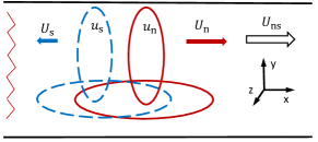
Figure 1: Schematics of the superfluid ⁴He channel counterflow. The normal-fluid eddies (solid red lines) and the superfluid eddies (the blue dashed lines) are swept by the corresponding mean velocities $U_{\text{n}}$ and $U_{\text{s}}$ away and towards the heater, respectively. The resulting counterflow velocity $U_{\text{ns}}$ is oriented along the positive $x$-direction. The streamwise-elongated eddies have longer overlap time than the cross-stream-elongated eddies.

The basic equations. The two-fluid model describes superfluid ⁴He of density $\rho$ as a mixture of two interpenetrating fluid components: an inviscid superfluid and a viscous normal-fluid. The densities of the components $\rho_{\text{s}},\rho_{\text{n}}:\rho_{\text{s}}+\rho_{\text{n}}=\rho$ define their contributions to the mixture. The fluid components are coupled by a mutual friction force, mediated by the tangle of quantum vortices Donnelly ; Vinen ; HV ; Vinen3 ; 37 of a core radius $a_{0}\approx 10^{-8}\,$cm and a fixed circulation $\kappa=h/M\approx 10^{-3}\,$cm²/s, where $h$ is Planck’s constant and $M$ is the mass of the ⁴He atom Feynman . A complex tangle of these vortex lines with a typical inter-vortex distance Vinen $\ell\sim 10^{-4}-10^{-2}\,$cm is a manifestation of superfluid turbulence.

To proceed it is sufficient to employ coarse-grained dynamics, following the gradually-damped versionHe4 of the Hall-Vinen-Bekarevich-Khalatnikov (HVBK) equations for counterflow turbulence He4 ; DNS-He4 ; LP-2018 ; DNS-He3 ; decoupling . It has a form of two Navier-Stokes equations for the turbulent velocity fluctuations ${\bm{u}}_{j}({\bm{r}},t)$ of the normal-fluid ($j=\rm n$) and the superfluid ($j=\rm s$):

$$\Big{[}\frac{\partial}{\partial t}+({\bm{u}}_{j}+{\bm{U}}_{j})\cdot{\bm{\nabla}}\Big{]}{\bm{u}}_{j}-\frac{{\bm{\nabla}}p_{j}}{\rho_{j}}=\nu_{j}\,\Delta{\bm{u}}_{j}+{\bm{f}}_{j}+{\bm{\varphi}}_{j},$$ (1)

coupled by the mutual friction forces ${\bm{f}}_{j}$ in the minimal form LNV : ${\bm{f}}_{\text{s}}\simeq\Omega_{\text{s}}\,({\bm{u}}_{\text{n}}-{\bm{u}}_{\text{s}})$, ${\bm{f}}_{\text{n}}\simeq\Omega_{\text{n}}\,({\bm{u}}_{\text{s}}-{\bm{u}}_{\text{n}})$, $\Omega_{\text{s}}=\alpha\kappa{\mathcal{L}}$, and $\Omega_{\text{n}}=\rho_{\text{s}}\Omega_{\text{s}}/\rho_{\text{n}}$. The mutual friction frequency $\Omega_{\text{s}}$ depends on the temperature-dependent dimensionless mutual friction parameter $\alpha(T)$ and on the vortex line density ${\mathcal{L}}$. In Eqs. (1) $p_{j}$ are the pressures of the normal-fluid and the superfluid components. The kinematic viscosity of the normal-fluid component is $\nu_{\text{n}}=\eta/\rho_{\text{n}}$ with $\eta$ being the dynamical viscosity of ⁴He DB98 . The energy sink in the equation for the superfluid component, proportional to the effective superfluid viscosity, $\nu_{\text{s}}$, accounts for the energy dissipation at the intervortex scale $\ell$, due to vortex reconnections and energy transfer to Kelvin waves Vinen ; He4 . The contributions, involving the reactive (dimensionless) mutual friction parameter $\alpha^{\prime}$, that renormalizes the nonlinear terms, were omitted due to its numerical smallness DB98 .

The large-scale motion in the thermal counterflow is sustained by the temperature gradient, created along the channel. Here we use the fact that the center of the channel flow at large enough Reynolds numbers can be considered as almost space-homogeneous Pope . To simplify the analysis we consider homogeneous turbulence under periodic boundary conditions and mimic the steering of turbulence at large scales by random forces ${\bm{\varphi}}_{j}$. Equations (1) describe the motion of two fluid components in the range of scales between the forcing scale and the intervortex distance.

Statistics of anisotropic turbulence. The most general description of homogeneous superfluid ⁴He turbulence at the level of second-order statistics can be done in terms of the three-dimensional (3D) Fourier-spectrum of each component and the cross-correlation functions:

$$(2\pi)^{3}\delta({\bm{k}}-{\bm{k}}^{\prime}){\mathcal{F}}^{\alpha\beta}_{ij}(\bm{k})=\left\langle v_{i}^{\alpha}(\bm{k})v_{j}^{*\beta}(\bm{k}^{\prime})\right\rangle,$$ (2)

where ${\bm{v}}_{j}({\bm{k}})$ is the Fourier transform of ${\bm{u}}_{j}({\bm{r}})$; the indices $i$ and $j$ refer to the fluid components; the vector indices $\alpha,\beta=\{x,y,z\}$ denote the Cartesian coordinates and ^∗ stands for complex conjugation. In the following, we choose the counterflow velocity, $U_{\text{ns}}=U_{\text{n}}-U_{\text{s}}$ along the $\hat{{\bm{x}}}$-direction as depicted in Fig.(1). Next denote the trace of any tensor according to ${\mathcal{F}}_{jj}(\bm{k})\equiv\sum_{\alpha}{\mathcal{F}}^{\alpha\alpha}_{jj}(\bm{k})$. With this notation, the kinetic energy density per unit mass ${\mathcal{E}}_{j}$ reads

$${\mathcal{E}}_{j}\equiv\frac{1}{2}\left\langle|{\bm{u}}_{j}({\bm{r}})|^{2}\right\rangle=\frac{1}{2}\int{\mathcal{F}}_{jj}(\bm{k})d^{3}k\big{/}(2\pi)^{3}\,.$$ (3)

Due to the presence of the preferred direction, defined by the counterflow velocity, the counterflow turbulence has an axial symmetry around the $\hat{{\bm{x}}}$ axis. Then ${\mathcal{F}}_{ij}({\bm{k}})$ depends only on the two projections $k_{\|}=k_{x}$ and $k_{\perp}=\sqrt{k_{y}^{2}+k_{z}^{2}}$ of the wave-vector ${\bm{k}}$, being independent of the angle $\phi$ in the $\perp$-plane, orthogonal to ${\bm{U}}_{\text{ns}}$. This allows us to define a set of two-dimensional (2D) objects that still contain all the information about 2${}^{\text{nd}}$-order statistics of the counterflow turbulence

$$F_{ij}(k_{\|},k_{\perp})\equiv\frac{k_{\perp}}{4\pi^{2}}{\mathcal{F}}_{ij}(k_{\|},k_{\perp})\ .$$ (4a)

Another way to represent the same information is to introduce a polar angle $$cos(\theta)=({\bm{k}},{\bm{U}}_{\text{ns}})/|{\bm{k}}||{\bm{U}}_{\text{ns}}|$$, and to use spherical coordinates:

$$\tilde{F}_{ij}(k,\theta)\equiv\frac{k}{4\pi^{2}}{\mathcal{F}}_{ij}(k\cos\theta,k\sin\theta)\ .$$ (4b)

Physical origin of the strong anisotropy. The physical origin of the strong anisotropy in the counterflow turbulence is best exposed by considering the balance equation for the 2D energy spectra $\tilde{F}_{\text{nn}}(k,\theta),\tilde{F}_{\text{ss}}(k,\theta)$. For that we start with Eqs. (1), follow the procedure described in  LABEL:LP-2018 and average the resulting equations for the 3D spectra over the azimuthal angle $\varphi$. Finally, for the normal component we get:

$$\frac{\partial\tilde{F}_{{\rm n}{\rm n}}(k,\theta,t)}{\partial t}\!+\!\mbox{div}_{{\bm{k}}}[{\bm{\varepsilon}}_{\rm n}({\bm{k}})]=-{\mathcal{D}}_{\rm n}^{\text{mf}}(k,\theta)\!-\!{\mathcal{D}}_{\rm n}^{\text{kv}}(k,\theta),$$

$${\mathcal{D}}_{\rm n}^{\text{mf}}(k,\theta)=\Omega_{\rm n}[\,\tilde{F}_{{\rm n}{\rm n}}(k,\theta)-\tilde{F}_{\text{ns}}(k,\theta)\big{]}\,,$$ (5)

$${\mathcal{D}}_{\rm n}^{\text{kv}}(k,\theta)=2\,\nu_{\rm n}k^{2}\,\tilde{F}_{{\rm n}{\rm n}}(k,\theta)\,,$$

where div${}_{{\bm{k}}}[{\bm{\varepsilon}}_{j}({\bm{k}})]$ is the transfer term due to inertial non-linear effects, ${\mathcal{D}}_{\rm n}^{\text{mf}}(k,\theta)$ describes the rate of energy dissipation by the mutual friction, while ${\mathcal{D}}_{\rm n}^{\text{kv}}(k,\theta)$ stands for the rate of dissipation by the kinematic viscosity. A similar equation is obtained for the superfluid component by replacing ${\rm n}$ with ${\rm s}$ everywhere.

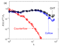
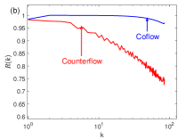
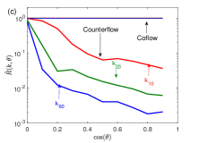
Figure 2: (a) The spherical energy spectra $E_{jj}(k)$ of the normal-fluid (circles) and the superfluid (squares), (b) the cross-correlation function $R(k)$ and (c) the angular dependence of the cross correlation function $\tilde{R}(k,\theta)$ for the coflow and the counterflow. In panel (c), the data for the coflow all coincide with the isotropic result. For the counterflow, red lines correspond to the $\tilde{R}(k,\theta)$ averaged over the wavenumber range $10\leq k<20$, green lines – to averaging over $20\leq k<60$ and blue lines – to the averaging over $60\leq k\leq 80$ (labeled as $k_{10}$, $k_{20}$, and $k_{60}$, respectively). Note the log-linear scale.

For a qualitative analysis of the origin of the anisotropy in our system it is important to develop a closure of the cross-correlation function $\tilde{F}_{\text{ns}}(k,\theta)$ in ${\mathcal{D}}_{j}^{\text{mf}}(k,\theta)$ in terms of the spectral properties of each fluid component and of the counterflow velocity.

According to LABEL:decoupling:

$$\tilde{F}_{\text{ns}}(k,\theta)=AB/[B^{2}+({\bm{k}}\cdot{\bm{U}}_{\text{ns}})^{2}]\ .$$ (6)

Here $A=\Omega_{\text{s}}\tilde{F}_{\text{nn}}(k,\theta)+\Omega_{\text{n}}\tilde{F}_{\text{ss}}(k,\theta)$ and $B$ can be approximated as $B=\Omega_{\text{n}}+\Omega_{\text{s}}$, as shown in LP-2018 . We further simplify $\tilde{F}_{\text{ns}}(k,\theta)$ in Eqs. (6) by noting LP-2018 that when two components are highly correlated, the cross-correlation may be accurately represented by the corresponding energy spectra. For wavenumbers where the components are not correlated, as is quantified by the decorrelation function $D(k,\theta)$ decoupling , $\tilde{F}_{\text{ns}}(k,\theta)$ is small and the accuracy of its representation is less important. We therefore get a decoupled form of the cross-correlation:

$$\tilde{F}_{\text{ns}}(k,\theta) = \tilde{F}_{jj}(k,\theta)D(k,\theta)\,,$$ (7a)

$$D(k,\theta) = \Big{[}1+\Big{(}\frac{kU_{\text{ns}}\cos\theta}{\Omega_{\text{n}}+\Omega_{\text{s}}}\Big{)}^{2}\Big{]}^{-1}\,,$$ (7b)

and finally determine the rate of energy dissipation due to mutual friction:

$${\mathcal{D}}_{j}^{\text{mf}}(k,\theta)=\Omega_{j}\tilde{F}_{jj}(k,\theta)\big{[}1-D(k,\theta)\big{]}\ .$$ (7c)

Equations (7) are the central analytical result of this paper.

The impact of $U_{\text{ns}}$ on the anisotropy follows from the closure (7c). Indeed, for small $k$ or even for large $k$ with ${\bm{k}}$ almost perpendicular to ${\bm{U}}_{\text{ns}}$ (i.e $\cos\theta\ll 1$), $D(k,\theta)\simeq 1$, the normal-fluid and superfluid velocities are almost fully coupled and the dissipation rate is small: ${\mathcal{D}}_{j}^{\text{mf}}(k,\theta)\ll\Omega_{j}$. In this case, the mutual friction does not significantly affect the energy balance and we expect the energy spectrum $\tilde{F}_{jj}(k,\theta)$ to be close to the Kolmogorov-1941 (K41) prediction $E_{\scriptscriptstyle\rm{K41}}(k)\propto k^{-5/3}$ for both components. For large $k$ and with $\cos\theta\sim 1$, the velocity components are almost decoupled $D(k,\theta)\ll 1$, and the mutual-friction energy dissipation is maximal: ${\mathcal{D}}_{j}^{\text{mf}}(k,\theta)\approx\Omega_{j}\widetilde{F}_{jj}(k,\theta)$. This situation is similar to that in ³He with the normal-fluid component at rest DNS-He3 . In such a case, we can expect that the energy dissipation by mutual friction strongly suppresses the energy spectra, much below the K41 expectation $E_{\scriptscriptstyle\rm{K41}}(k)$.

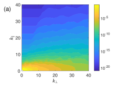
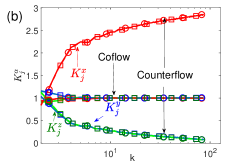
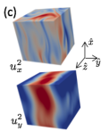
Figure 3: (a)The superfluid component energy spectrum $F_{\text{ss}}(k_{\|},k_{\perp})$ in the counterflow. (b) The tensor decomposition of the normalized spherical energy spectra $K_{j}^{\alpha}(k)$ for the normal-fluid (circles) and the superfluid (squares). (c) The superfluid velocity components ${\bm{u}}_{\rm s}^{x}({\bm{r}})$(top) and ${\bm{u}}_{\rm s}^{y}({\bm{r}})$(bottom). The ${\bm{u}}_{\rm s}^{z}({\bm{r}})$ (not shown) is similar to ${\bm{u}}_{\rm s}^{y}({\bm{r}})$. The velocity magnitude is color-coded with red denoting positive and blue denoting negative values.

Combining all these considerations, we expect the energy spectra $\tilde{F}_{jj}(k,\cos\theta)$ to become more anisotropic with increasing $k$, with most of the energy concentrated in the range of small $\cos\theta$, i.e. in the orthogonal plane.

Numerical results. Direct numerical simulations of the coupled HVBK Eqs. (1) were carried out using a fully de-aliased pseudospectral code with a resolution of $256^{3}$ collocation points in a triply periodic domain of size $L=2\pi$. To reach a steady state flow, velocity fields of the normal and superfluid components are stirred by two independent random Gaussian forces ${\bm{\varphi}}_{\text{s}}$ and ${\bm{\varphi}}_{\text{n}}$ with the force amplitudes $|\varphi|=0.5$ for both components, localized in the band $k_{\varphi}\in[0.5,1.5]$. The time integration is performed using 2-nd order Adams-Bashforth scheme with viscous term exactly integrated.

We have decided to focus on the temperature $T=1.85$ K, at which the densities and viscosities of the normal-fluid and superfluid components are close: $\rho_{\text{s}}/\rho_{\text{n}}=1.75$ and $\nu_{\text{s}}/\nu_{\text{n}}=1.07$. The mutual friction parameter for this temperature is $\alpha=0.18$. The simulations were carried out with both the normal-fluid and superfluid viscosity $\nu_{\text{n}}=\nu_{\text{s}}=0.003$. Other parameters of the simulations were chosen based on the relevant dimensionless relations: the Reynolds numbers and the normal-fluid turbulent intensity $w$

$$Re_{j}=(u^{j}_{\scriptscriptstyle\rm{T}})(/\nu_{j}k_{0})\,,\quad w=U_{\text{ns}}/u^{\text{n}}_{\scriptscriptstyle\rm{T}}\,.$$ (8)

Here $u^{j}_{\scriptscriptstyle\rm{T}}=\sqrt{\langle{u_{j}}^{2}\rangle}$ is the root mean square (rms) of the turbulent velocity fluctuations, $k_{0}=1$ is the outer scale of turbulence. To emphasize the importance of the counterflow, we compare the results with the simulations for the so-called coflow with the rest of the parameters being the same. In the coflow, the two components of the mechanically driven ⁴He, being coupled by the mutual friction force, move in the same direction with the same mean velocities, $U_{\text{ns}}=0$. The statistics in the coflow configuration is known to be similar to that of classical isotropic turbulence DNS-He4 ; TenChapters ; BLR ; Roche-new . In our simulations, the values of the Reynolds numbers in the counterflow are $Re_{\text{n}}=1051$ and $Re_{\text{s}}=1056$, while in the coflow, $Re_{\text{n}}=1179$ and $Re_{\text{s}}=1181$. The rms velocities of both components in both flows are $u^{\text{s}}_{\scriptscriptstyle\rm{T}}=u^{\text{n}}_{\scriptscriptstyle\rm{T}}=3.5$. The dimensionless values of the mutual friction frequency $\Omega_{\text{s}}=20$ and the counterflow velocity $U_{\text{ns}}=15.4$ correspond to the case with both components strongly turbulent and strongly coupled. The results on the temperature and $\Omega_{\text{s}}$ dependence of the energy spectra will be reported elsewhere. The flow conditions were controlled by the simulations of the uncoupled equations without counterflow (${\bm{U}}_{j}=\Omega_{j}=0$), which represent here the classical hydrodynamic isotropic turbulence (CHT).

The energy spectra are influenced by the viscous dissipation, by the dissipation due to mutual friction and by the counterflow-induced decoupling. To clarify the role of each of these factors, we first ignore the expected anisotropy and compare in Fig. 2(a) the normal-fluid and superfluid energy spectra $E_{\text{nn}}(k)$ and $E_{\text{ss}}(k)$ and the cross-correlation $E_{\text{ns}}(k)$, integrated over a spherical surface of radius $k$, i.e. over all directions of vector ${\bm{k}}$:

$$E_{ij}(k)=\int{\mathcal{F}}_{ij}({\bm{k}})\,\frac{d\phi\,d\cos\theta}{(2\pi)^{3}}\ .$$ (9)

The corresponding normalized cross-correlation functions

$$R(k)=2\,E_{\text{ns}}(k)/[E_{\text{nn}}(k)+\,E_{\text{ss}}(k)]$$ (10)

are shown in Fig. 2(b). The effect of viscous dissipation is clearly seen in the spectra of the uncoupled components, corresponding to classical hydrodynamic turbulence (marked “CHT”, black lines). The spectra almost coincide, since at $T=1.85$ K the viscosities are close. In the coflow, the strongly coupled components are well correlated at all scales and move almost as one fluid. Note the additional dissipation due to mutual friction, leading to further suppression of the spectra compared to the uncoupled case. The presence of the counterflow velocity leads to a sweeping decoupling of the two component’s eddies in opposite directions by the corresponding mean velocities. The result is the decorrelation of the components turbulence velocities, especially at small scales, for which the overlapping time is very short, see Fig. 2(b). The dissipation by mutual friction is very strong in this case, with both $\Omega$ and the velocity difference being large, leading to very strongly suppressed spectra, with $E_{\text{nn}}(k)\approx E_{\text{ss}}(k)$. This behavior was predicted by the theory LP-2018 , based on the assumption of spectral isotropy. However the spherically integrated spectra and cross-correlations cannot reveal any properties connected to the anisotropic action of the mutual friction force. To account for the spectral anisotropy we plot in Fig. 2(c) the normalized 2D cross-correlations

$$\tilde{R}(k,\theta)=2\tilde{F}_{\text{ns}}(k,\theta)/[\tilde{F}_{\text{nn}}(k,\theta)+\tilde{F}_{\text{ss}}(k,\theta)].$$ (11)

Given the discrete nature of the ${\bm{k}}$-space in DNS, we average them over 3 bands of wavenumbers. Leaving aside $k\approx k_{0}$, influenced by the forcing, we average $\tilde{R}(k,\theta)$ over the $k$-ranges $10\leq k<20$, $20\leq k<60$ and $60\leq k\leq 80$.

The first observation here is that the cross-correlation for the coflow are isotropic at all scales, see thin horizontal lines, marked “coflow”. On the other hand, in the counterflow, the cross-correlations are largest for $\cos\theta\approx 0$ and fall off very fast with decreasing angle, slower for small $k$ (red lines, labelled $k_{10}$) and faster as $k$ become larger (green, $k_{20}$, and blue lines, $k_{60}$, respectively). Such a strong decorrelation of the components velocities leads to an enhanced dissipation by mutual friction in the counterflow direction, such that most of the energy is contained in the narrow range $\cos\theta\lesssim 0.1$, near the plane orthogonal to ${\bm{U}}_{\text{ns}}$.

Indeed, the superfluid energy spectrum $F_{\text{ss}}(k_{\|},k_{\perp})$, shown in Fig. 3(a), is strongly suppressed in the $k_{||}$ direction, while it decays slowly in the orthogonal plane. A similar phenomenon of the creation of quasi-2D turbulence is observed in a strongly stratified atmosphere AtmTurb-review ; 2018-AB ; atmosTurb-Kumar and in rotating turbulence rot1 ; rot2 ; rot3 , in which there exists a preferred direction defined by gravity or by a rotation axis. The difference between these examples and the present counterflow lies in the nature of the velocity field. The leading velocity components in the classical flows are in a plane orthogonal to the preferred direction. Moreover, at small scales the isotropy is restored atmosTurb-Kumar ; 2018-AB . On the contrary, in ⁴He counterflow, the dominant velocity component is oriented along the counterflow direction, with the anisotropy becoming stronger with decreasing scales, as we show in Fig. 3(b). Here we plot the tensor components of the spherical spectra as the ratios

$$K_{j}^{\alpha}(k)\equiv 3\,E^{\alpha\alpha}_{jj}(k)/\,E_{jj}(k).$$ (12)

The factor 3 was introduced to ensure that for isotropic turbulence $K_{j}^{\alpha}(k)=1$. Expectedly, the coflow (the almost horizontal lines) is isotropic at all scales, except for the smallest wavenumbers. On the other hand, for the counterflow turbulence, the contribution of the $K_{j}^{x}(k)$ component (shown by red lines) is dominant and monotonically increases with $k$ from the isotropic level $K_{j}^{x}(k_{0})\approx 1$ to the maximal possible level $K_{j}^{x}(k)\approx 3$. Therefore the small-scale counterflow turbulence consists mainly of $v_{j}^{x}(k)$ velocity fluctuations. The contribution of $v_{j}^{y}$ and $v_{j}^{z}$ fluctuations for $k\gtrsim 10$ is negligible. Summarizing Fig. 3, the leading contribution to the spectra of small scale counterflow turbulence comes from the turbulent velocity fluctuations with only one stream-wise projection that depends on the two cross-stream coordinates $\{y,z\}$: $u^{x}(y,z)$. Such type of turbulence can be visualized as narrow jets or thin sheets with velocity, oriented along the counterflow and randomly distributed in the $\perp$-plane. Indeed the velocity components $u^{y}_{\rm s}$, shown in Fig. 3c, and $u^{z}_{\rm s}$ have only large scale structures, while $u^{x}_{\rm s}$ has elongated structures at various scales. The energy spectra, corresponding to $u^{x}_{\rm n}(y,t)$ were recently measured experimentally WG-2017 ; WG-2018 and were found to agree with predictions LP-2018 in the range of scales where the fluid components are well correlated, while decaying faster than predicted at smaller scales.

Summary. The energy spectra of the superfluid ⁴He counterflow turbulence become more anisotropic upon going from large scales toward scales about the intervortex distance. This strong anisotropy distinguish it from the classical turbulent flows that become more isotropic as the scale decreases. Most of the turbulent energy become concentrated in the plane, orthogonal to the counterflow direction. Furthermore, contrary to classical quasi-2D turbulent flows in rotation or in stratified configurations, where dominant velocity components lie in the same plane, the only surviving velocity component at small scales is preferentially oriented along the counterflow direction. The selective suppression of the orthogonal velocity fluctuations has its origin in the strong anisotropy of the energy dissipation by mutual friction, resulting from the angular dependence of the components’ cross-correlation.

Acknowledgments LB acknowledges funding from the European Unions Seventh Framework Programme (FP7/20072013) under Grant Agreement No. 339032. GS thanks AtMath collaboration at University of Helsinki. DK acknowledges funding from the Simons Foundation under grant No. 454955 (Francesco Zamponi).

References

- (1) L. Biferale and I. Procaccia, Phys. Rep. 414 43, (2005).
- (2) U. Frisch, Turbulence, the legacy of A.N. Kolomogorov, Cambridge Univ. Press, 1995.
- (3) R. J. Donnelly, Physics Today 62, 34 (2009).
- (4) R. J. Donnelly, Quantized Vortices in Hellium II (Cambridge 3 University Press, Cambridge, 1991).
- (5) W. F. Vinen and J. J. Niemela, J. Low Temp. Phys. 128, 167 (2002).
- (6) H. E. Hall and W. F. Vinen, Proc. Roy. Soc. A 238, 204 (1956).
- (7) W. F. Vinen, Proc. R. Soc. 240, 114 (1957); 240, 128 (1957); 242, 493 (1957); 243, 400 (1958).
- (8) R. N. Hills and P. H. Roberts, Arch. Ration. Mech. Anal. 66, 43 (1977).
- (9) Quantized Vortex Dynamics and Superfluid Turbulence, edited by C.F. Barenghi, R.J. Donnelly and W.F. Vinen, Lecture Notes in Physics 571 (Springer-Verlag, Berlin, 2001)
- (10) R. P.Feynman, Progress in Low Temperature Physics 1, 17 (1955).
- (11) L. Boue, V.S. L’vov, Y. Nagar, S.V. Nazarenko, A. Pomyalov, I. Procaccia, Phys. Rev. B. 91, 144501, (2015).
- (12) D. Khomenko, V. S. L’vov, A. Pomyalov, and I. Procaccia, Phys. Rev. B 93, 014516 (2016).
- (13) L. Biferale, D. Khomenko, V. L’vov, A. Pomyalov, I. Procaccia and G. Sahoo, Phys. Rev. B. 95, 184510 (2017).
- (14) L. Biferale, D. Khomenko, V.S. L’vov, A. Pomyalov, I. Procaccia, and G. Sahoo, Phys. Rev.Fluids 3, 024605 (2018).
- (15) V. S. L’vov and A. Pomyalov, Phys. Rev. B, 97, 214513 (2018).
- (16) V. S. L’vov, S. V. Nazarenko and G. E. Volovik, JETP Letters, 80, 535 (2004).
- (17) R. J. Donnelly, C. F. Barenghi , J. Phys. Chem. Ref. Data 27, 1217(1998).
- (18) S. B. Pope, Turbulent Flows (Cambridge University Press, Cambridge, 2000).
- (19) L. Skrbek and K. R. Sreenivasan, in Ten Chapters in Turbulence, edited by P. A. Davidson, Y. Kaneda, and K. R. Sreenivasan (Cambridge University Press, Cambridge, 2013), pp. 405–437.
- (20) C. F. Barenghi, V. S. L’vov, and P.-E. Roche, Proc Natl Acad Sci USA 111, 4683 (2014).
- (21) E. Rusaouen, B. Chabaud, J. Salort, Philippe-E. Roche. Physics of Fluids 29, 105108 (2017).
- (22) E.J. Hopfinger, J Geophys Res. 92,5287(1987).
- (23) A. Kumar, M. K. Verma and J. Sukhatme, J. of Turbulence, 18, 219(2017).
- (24) A. Alexakis, L. Biferale, Phys. Rep. 767-769,1 (2018).
- (25) L. Biferale, F. Bonaccorso, I. M. Mazzitelli, M. A. T. van Hinsberg, A. S. Lanotte, S. Musacchio, P. Perlekar, and F. Toschi. Phys. Rev. X 6, 041036 (2016).
- (26) B. Gallet, A. Campagne, P.-P. Cortet, and F. Moisy, Phys. Fluids 26, 035108 (2014).
- (27) . B. Gallet, J. Fluid Mech. 783, 412 (2015).
- (28) J. Gao, E. Varga, W. Guo and W. F. Vinen, Phys. Rev. B 96, 094511 (2017).
- (29) S. Bao, W. Guo, V. S. L’vov, A. Pomyalov, Phys. Rev. B 98, 174509 (2018).