Evaluating topological charge density with symmetric multi-probing method

Abstract

We evaluated the topological charge density of SU(3) gauge fields on lattice by calculating the trace of overlap Dirac matrix employing symmetric multi-probing(SMP) method with 3 modes. Since the topological charge $Q$ for a given lattice configuration must be an integer number, it’s easy to estimate the systematic error (the deviation of $Q$ to nearest integer). The results showed high efficiency and accuracy in calculating the trace of the inverse of a large sparse matrix with locality by using SMP sources, compared with that using point sources. We also showed the correlation between the errors and probing scheme parameter $r_{\mathrm{min}}$ as well as lattice volume $N_{L}$ and lattice spacing $a$. It was found that the computing time of calculating the trace by employing SMP sources is less dependent on $N_{L}$ than that by using point sources. Therefore the SMP method is very suitable for calculations on large lattices.

1.15.Ha, 02.10.Yn

1 introduction

Topological charge $Q$ and density $q\left(x\right)$ are important quantities to the investigation of the structure of quantum chromodynamics(QCD) vacuum, and the susceptibility of $Q$ is related to $\eta^{\prime}$ mass by Witten-Veneziano relation [1, 2]. Lattice QCD is one of the best non-perturbative framework to study QCD properties, in which space-time is discretized on lattice. $Q$ on lattice can be calculated by gauge field tensor $F_{\mu\nu}$ [3]:

$$Q=\int\mathrm{d}^{4}xq\left(x\right)=\frac{1}{32\pi^{2}}\int\mathrm{d}^{4}x\mathrm{tr}\left(\epsilon_{\mu\nu\rho\sigma}F_{\mu\nu}F_{\rho\sigma}\right),$$ (1)

where the trace is over color indexes, and $\epsilon_{\mu\nu\rho\sigma}$ is a totally antisymmetric tensor. However, the topological charge $Q$ calculated in this way is always not an integer unlike that in the continuum, unless multiplied by a renormalization factor or calculated on smoothed configurations whose renormalization factor tends to 1. Smoothing methods or other cooling-like methods will change the topological density, and also introduce ambiguous smoothing parameter like smoothing time $n_{\mathrm{sm}}$ which is always set empirically. Another way to get $q\left(x\right)$ is evaluating the trace of chiral Dirac fermion operator in Dirac and color space [4]:

$$q\left(x\right)=\frac{1}{2}\mathrm{tr}\left(\gamma_{5}D_{\mathrm{chiral}}\right),$$ (2)

where the trace is over color and Dirac indexes, $\gamma_{5}$ is Dirac gamma matrix, and $D_{\mathrm{chiral}}$ is a chiral Dirac fermion operator on lattice. In this definition, $Q$ will be always an integer due to Atiya-Singer index theorem [5], but hard to be exactly calculated as evaluating the trace of $D_{\mathrm{chiral}}$ is a very expensive task. As one of the chiral Dirac fermions, overlap fermion operator [6, 7] is widely used in the studies of chiral properties of lattice QCD. Massless overlap Dirac operator $D_{\mathrm{ov}}$ is constructed by a kernal operator, usually using Wilson Dirac operator $D_{\mathrm{W}}$ as the kernal:

$$D_{\mathrm{ov}}=1+\gamma_{5}\epsilon\left(\gamma_{5}D_{\mathrm{W}}\right),$$ (3)

where the hopping parameter $\kappa$ in the kernal $D_{\mathrm{W}}$ is only a free parameter not related to bare quark mass, and $\kappa\in\left(\kappa_{c},0.25\right)$ with $\kappa_{c}$ refer to critical hopping parameter in Wilson fermion. We took $\kappa=0.21$ in this work. $\epsilon\left(\gamma_{5}D_{W}\right)$ is the sign function here:

$$\epsilon(\gamma_{5}D_{\mathrm{W}})=\mathrm{sign}\left(\gamma_{5}D_{\mathrm{W}}\right)=\frac{\gamma_{5}D_{\mathrm{W}}}{\sqrt{D_{\mathrm{W}}^{\dagger}D_{\mathrm{W}}}}=\gamma_{5}D_{W}\left(c_{0}+\sum_{i=1}^{\infty}\frac{c_{i}}{D_{\mathrm{W}}^{\dagger}D_{\mathrm{W}}+q_{i}}\right),$$ (4)

in which Zolotarev series expansion [8] is introduced. In our work 14th-order Zolotarev expansion was applied  [9]. To extract the trace of $D_{\mathrm{ov}}$, we need to calculate the trace of $D_{\mathrm{W}}^{-2}$, while $D_{\mathrm{W}}$ is a large sparse matrix. Its rank is $12N_{L}$, where $N_{L}$ is the number of lattice sites, empirically in a range of $10^{5}\sim 10^{8}$ depending on the lattice size. So the trace of $D_{\mathrm{W}}^{-2}$ is too expensive to calculate exactly.

Fortunately $D_{\mathrm{ov}}$ is a local operator [10], and there are methods to approximately calculate the trace of it by making use of this property. Multi-probing method is one of these methods  [11, 12] that can be used to estimating the trace of the inverse of a large sparse matrix when the inverse exhibits locality. A. Stathopoulos et al. developed the hierarchical multi-probing method and tested it in lattice QCD Monte Carlo calculation [13]. E. Endress et al. used multi-probing method to tackle the noise-to-signal problems when calculating all-to-all propagator in lattice QCD [14, 15] by applying the Greedy Multicoloring Algorithm to construct the multi-probing source vectors. Their results have showed the validity and efficiency of probing method.

In this work we employed symmetric multi-probing(SMP) method to evaluating the topological charge density by calculating $\mathrm{tr}\left(\gamma_{5}D_{\mathrm{ov}}\right)$, and showed its efficiency comparing to point source method. We will introduce the topological charge density as well as the trace calculation with point sources and SMP sources in next section. After that, calculation results will be presented and discussed. We will summarize our work in the last section.

2 methods

2.1 Topological charge density and trace calculation with point source

Overlap Dirac operator $D_{\mathrm{ov}}\left(x,y\right)_{\alpha\beta,ab}$ on a lattice $L(n_{x},n_{y},n_{t},n_{z})$ is a large sparse matrix, where $n_{\mu}$ denotes the number of sites in $\mu$ direction and $\mu=x,y,z,t$, $\alpha$ $\beta$ are Dirac indexes and $a$ $b$ are color indexes. The topological charge density $q\left(x\right)$ can be obtained by calculating the trace of massless overlap Dirac operator:

$$q(x)=\frac{1}{2}\mathrm{tr}_{\mathrm{d,c}}\left(\gamma_{5}D_{\mathrm{ov}}\left(x,x\right)\right)=\frac{1}{2}\sum_{\alpha,a}\left\langle\psi\left(x,\alpha,a\right)\right|\gamma_{5}D_{\mathrm{ov}}\left|\psi\left(x,\alpha,a\right)\right\rangle,$$ (5)

where the trace is over Dirac and color indexes, $|\psi(x,\alpha,a)\rangle$ is a normalized point source vector which has $N_{L}\times N_{d}\times N_{c}$ components where the lattice volume $N_{L}=n_{x}n_{y}n_{z}n_{t}$, $N_{d}=4$, $N_{c}=3$. Only one specific $\left(x,\alpha,a\right)$ component takes nonzero value in the point source. Substituting Eq. (3) and Eq. (4) into Eq. (5), the most expensive step to calculate the trace of $D_{\mathrm{ov}}$ is computing the multiplication:

$$v_{i}=\frac{c_{i}}{D_{\mathrm{W}}^{\dagger}D_{\mathrm{W}}+q_{i}}\left|\psi\left(x,\alpha,a\right)\right\rangle,$$ (6)

which is equivalent to solve the following linear equation:

$$M_{i}v_{i}=b,$$ (7)

where

$$M_{i}=\frac{1}{c_{i}}\left(D_{\mathrm{W}}^{\dagger}D_{\mathrm{W}}+q_{i}\right),\ b=\left|\psi\left(x,\alpha,a\right)\right\rangle.$$ (8)

This equation is expensive to solve for a large matrix $M_{i}$, and the huge number of point sources corresponding to sites on the whole lattice makes things even worse. The computing time to solve Eq. (7) with Conjugated Gradient(CG) algorithm for one source is more than $\mathcal{O}\left(N_{L}\right)$ (in consideration of that $M_{i}$ is a large sparse matrix, and its conditional number grows as $N_{L}$ grows), and there are $12N_{L}$ point sources. So the cost of evaluating $Q=\sum_{x}q\left(x\right)$ by calculating the trace of $D_{\mathrm{ov}}$ with point sources will be larger than $\mathcal{O}\left(N_{L}^{2}\right)$, which is too expensive especially for large $N_{L}$ [16, 17], although it’s the exact measurement of topological charge density on lattice without any approximation.

2.2 Trace calculation with multi-probing source

We know from above that calculation of the trace of $D_{\mathrm{ov}}$ with point source is a quite expensive task. Introduce a new source vector $\phi$ by adding two point sources:

$$\phi\left(x,y,\alpha,a\right)=\psi\left(x,\alpha,a\right)+\psi\left(y,\alpha,a\right),\ x\neq y,$$ (9)

then Eq. (5) can be rewritten as:

$$q(x) = \sum_{\alpha,a}\psi\left(x,\alpha,a\right)\tilde{D}_{\mathrm{ov}}\phi\left(x,y,\alpha,a\right)$$ (10)

$$-\sum_{\alpha,a}\psi\left(x,\alpha,a\right)\tilde{D}_{\mathrm{ov}}\psi\left(y,\alpha,a\right),$$

where $\tilde{D}_{\mathrm{ov}}=\frac{1}{2}\gamma_{5}D_{\mathrm{ov}}$, and the second term:

$$\sum_{\alpha,a}\psi\left(x,\alpha,a\right)\tilde{D}_{\mathrm{ov}}\psi\left(y,\alpha,a\right)=\sum_{\alpha,a}\tilde{D}_{\mathrm{ov}}(x,\alpha,a;y,\alpha,a)$$ (11)

are space-time off-diagonal elements of $D_{\mathrm{ov}}$. Considering the space-time locality of $D_{\mathrm{ov}}$, it has upper bound  [10, 16]:

$$\left|D_{\mathrm{ov}}\left(x,\alpha,a;y,\beta,b\right)\right|\leq C\exp\left(-\gamma\left|x-y\right|\right),$$ (12)

where $C$ and $\gamma$ are constants irrelevant to gauge field configurations, and $\left|x-y\right|$ is defined as the distance between site $x$ and site $y$. Note that $\gamma_{5}$ only exchanges the elements of $D_{\mathrm{ov}}$ in Dirac space, so $\tilde{D}_{\mathrm{ov}}$ also satisfies this inequation. ’off-diagonal’ will refer to ’space-time off-diagonal’ in the following unless otherwise stated. We checked this relation on several lattice configurations, as Fig. 1 shown. $\gamma$ in the inequation (12) is around $1.076$ by [16] where $\left|x-y\right|$ is defined as Euclid distance, and around $0.529$ as taxi driver distance. The result means that the off-diagonal elements of $D_{\mathrm{ov}}$ are exponentially suppressed as $\left|x-y\right|$ increases, and the inequation (12) holds when the distance is not too small (larger than 3) for two definitions of distance. We can also see that $\gamma$ for Euclid distance is larger which means stronger locality, so we adopted this definition in our work.

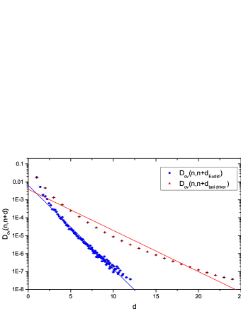
Figure 1: The locality of $D_{\mathrm{ov}}$ is shown by its averaged off-diagonal elements as a function of Euclid distance and taxi driver distance with logarithmic coordinates. Red line fits the taxi driver distance function with the slope $-0.528$, while blue line fits the Euclid distance function with the slope $-1.075$ in a lattice configuration.

So the approximate topological charge density $q\left(x\right)$ can be written as:

$$q^{\mathrm{approx}}(x) = \sum_{\alpha,a}\psi(x,\alpha,a)\tilde{D}_{\mathrm{ov}}\phi(x,y,\alpha,a),$$ (13)

$$q^{\mathrm{approx}}(y) = \sum_{\alpha,a}\psi(y,\alpha,a)\tilde{D}_{\mathrm{ov}}\phi(x,y,\alpha,a).$$ (14)

We can see that the approximate density of both sites can be easily calculated from $\tilde{D}_{\mathrm{ov}}\phi(x,y,\alpha,a)$, so only one linear equation like Eq. (7) need to be solved to obtain $q\left(x\right)$ and $q\left(y\right)$ as long as $\left|x-y\right|$ is sufficiently large. This method is called as multi-probing method or probing method.

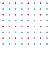
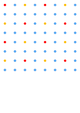
Figure 2: Example of Split Mode on $8\times 8$ 2-D lattice. Red sites in the left panel are colored in Normal Mode coloring scheme $P(4,4,0)$, and in the right panel they split into two subsets with red and yellow color in Split Mode scheme $P(4,4,1)$.

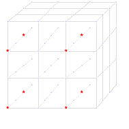
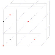
Figure 3: Examples of Split Mode on $4^{3}$ 3-D lattice. sites denoted as red stars in the left panel are colored in Normal Mode coloring scheme $P(2,2,2,0)$, while in the right panel they split into two subsets, red stars and black triangles in Split Mode scheme $P(2,2,2,1)$.

We firstly mark all sites in the lattice with a color label, called coloring algorithm. The sites with the same color form a subset of the whole lattice sites set. Then one multi-probing source can be constructed by a subset as follow: choose a color and Dirac index, construct point sources on sites in the subset and add all these point source vectors.

In order to reduce the calculation cost, we would like to reduce the number of MP sources by combining more point sources in one MP source. However, the errors introduced by MP source will exponentially depend on the distance between the sites in the subset, as Eq. (12) shown. We should include the sites that as far away as possible from each other in one MP source to control the systematic errors. Therefore appropriate coloring algorithm is important to optimize the balance of the systematic errors and calculation cost.

We chose a symmetric coloring algorithm and Euclid distance definition in this work, which marks the sites with same color in each direction with fixed distance. There are other algorithms like GCA(Greedy coloring Algorithm) [12] who used taxi driver distance definition. It’s convenient to choose the same gap $r$ in each direction, then the minimal distance of each two sites in the subsets $r_{\mathrm{min}}=r$. We call this type of MP sources by Normal Mode, as we show some examples in left panel of Fig. 2 and Fig. 3.

Furthermore, we can divided a subset into two subsets by marking half of sites with a new color, while each site has different color with its neighbors, see examples in Fig. 2 and Fig. 3 on 2-D and 3-D lattices. In this Split Mode, $r_{\mathrm{min}}^{\prime}=\sqrt{2}r$ for the two new subsets.

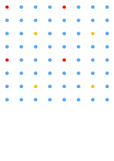
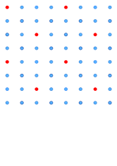
Figure 4: Example of combined mode on $8\times 8$ 2-D lattice. Red sites and yellow sites in the left panel are two subsets colored in normal symmetric coloring scheme $P(2,2,0)$, and in the right panel they are combined into one with red color in combined mode scheme $P(2,2,2)$. Note that the minimal distance changes from $4$ to $2\sqrt{2}$.

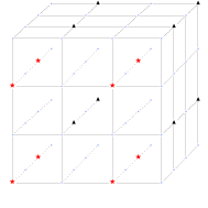
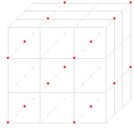
Figure 5: Example of combined mode on $4^{3}$ 3-D lattice. Red stars and black triangles in the left panel are two subsets colored in normal symmetric coloring scheme $P(2,2,2,0)$, and in the right panel they are combined into one note by red stars in combined mode scheme $P(2,2,2,2)$. Note that the minimal distance changes from $2$ to $\sqrt{3}$.

We can also combine two subsets into a new subset which include two sites with the space-time offset equals $(r/2,r/2,r/2,r/2)$, then the minimal distance remains unchanged, that is $r_{\mathrm{min}}^{\prime}=r$ for the new subset. We call this mode by Combine Mode, while number of sites doubles and errors are increased due to more nearest neighbors are introduced. Note that this combined mode only works on 4-D lattices , and $r$ should be even. Fig. 4 and Fig. 5 show examples of Combine Mode in 2D and 3D situations, while $r_{\mathrm{min}}=r/\sqrt{2}$ and $r_{\mathrm{min}}=\sqrt{3}r/2$ respectively after combination.

Considering this on a lattice $L(n_{x},n_{y},n_{z},n_{t})$. Firstly choose a symmetric coloring scheme $P\left(m_{x,}m_{y},m_{z},m_{t},\mathrm{mode}\right)$, which means $m_{\mu}$ sites are marked with same color in $\mu$ direction of the lattice, and the mode label can be $0,1,2$ which respectively means Normal, Split and Combine Mode. Then pick a site $X(x_{1},x_{1},x_{3},x_{4})$ as a seed site with $x_{\mu}$ denotes its coordinate on the lattice, we can construct a SMP source $\phi_{P}$ in scheme $P\left(m_{x,}m_{y},m_{z},m_{t},\mathrm{mode}\right)$:

$$\phi_{P}\left(S\left(X,P\right),\alpha,a\right)=\sum_{y\in S\left(X,P\right)}\psi\left(y,\alpha,a\right),$$ (15)

where $S\left(X,P\right)$ denotes the site subset that including all sites with the same color of site $X$ by coloring scheme $P\left(m_{x,}m_{y},m_{z},m_{t},\mathrm{mode}\right)$.

The topological charge density on any site $x\in S\left(X,P\right)$ can be calculated by this combined source:

$$q^{\mathrm{approx}}(x)=\sum_{\alpha,a}\psi(x,\alpha,a)\tilde{D}_{\mathrm{ov}}\phi_{{}_{P}}\left(S\left(X,P\right),\alpha,a\right)=q(x)+\sum_{\alpha,a}\sum_{y\in S(X,P)}^{y\neq x}\tilde{D}_{\mathrm{ov}}(x,\alpha,a;\ y,\alpha,a),$$ (16)

the second term sums the corresponding off-diagonal components of $D_{\mathrm{ov}}$, which satisfy Eq. (12).

Now the whole lattice sites can be divided into $N^{\mathrm{SMP}}$ site sets, with $m_{x}m_{y}m_{z}m_{t}$ sites in each set for $\mathrm{mode}=0$ or $\frac{1}{2}m_{x}m_{y}m_{z}m_{t}$ sites for $\mathrm{mode}=1$, $2\times m_{x}m_{y}m_{z}m_{t}$ sites for $\mathrm{mode}=2$. Each site on the lattice should belong to and only belong to one set in a specific scheme $P$. SMP sources are constructed from these symmetric site sets that only distinct from each other with some units of coordinate shift. In this case all SMP sources include the same number of sites for a specific $P$, which leads to less sources needed compared with Greedy Multicoloring Algorithm for the same minimal Euclid distance $\left|x-y\right|$. Summing Eq. (16) over the lattice volume, the total introduced systematic error of $Q$ will be:

$$R_{P} = Q^{\mathrm{approx}}-Q=\sum_{x\in V}\sum_{\alpha,a}\sum_{y\in S(x,P)}^{y\neq x}\tilde{D}_{\mathrm{ov}}^{-1}(x,\alpha,a;\ y,\alpha,a)$$ (17)

$$\leq 6N_{L}C\sum_{y\in S(x,P)}^{y\neq x}\exp\left(-\gamma\left|x-y\right|\right),$$

where Eq. (12) is used and the sum over color and Dirac indexes results a factor of $12$. In practice the errors are far smaller than its upper bound. Define the minimal distance $r_{\mathrm{min}}^{P}$ for a SMP scheme $P$, which is the minimal Euclid distance of any two sites in a site set $S\left(X,P\right)$ based on arbitrary seed site $X$:

$$r_{\mathrm{min}}^{P}=\mathrm{min}\left\{\left|x-y\right|,\forall x,y\in S\left(X,P\right),\ x\neq y\right\},$$ (18)

we believe that $\left|x-y\right|=r_{\mathrm{min}}^{P}$ terms will dominate in Eq. (17).

For the case of a spatial symmetric lattice $L\left(n_{s},n_{s},n_{s},n_{t}\right)$, the SMP scheme can be chosen as $P\left(\frac{n_{s}}{r},\frac{n_{s}}{r},\frac{n_{s}}{r},\frac{n_{t}}{r},\mathrm{mode}\right)$ so that

$$r_{\mathrm{min}}=\begin{cases}r,&\mathrm{mode}=0,2\\ r\sqrt{2},&\mathrm{mode}=1.\end{cases}$$ (19)

Therefore the choice of $r_{\mathrm{min}}$ should be one of the common factors of $n_{s}$ and $n_{t}$, or multiplied by $\sqrt{2}$ when $\mathrm{mode}=1$, such as $r_{\mathrm{min}}=2$ in the left panel of Fig. 2, and $r_{\mathrm{min}}=2\sqrt{2}$ in the right panel. We chose appropriate $r_{\mathrm{min}}$ and SMP schemes for different lattices in this way.

3 Lattice setup and results

We calculated topological charge density and the total topological charge for pure gauge lattice configurations with Iwasaki gauge action [18]:

$$S_{\mathrm{IA}}=\beta c_{1}\left\{\Omega_{p}+r_{\beta}\Omega_{r}\right\}$$ (20)

where $\beta$ is the bare coupling constant, $\Omega_{C}=\sum\frac{1}{3}\mathrm{ReTr}\left(1-W_{C}\right)$ is the real part of the trace over all Wilson loop $W_{C}$ with closed contour $C$, while subscripts $p$ and $r$ refer to plaquette and $2\times 1$ rectangle respectively. $c_{1}=3.648$, $r_{\beta}=-0.09073465$ in Iwasaki action which is an $\mathcal{O}\left(a^{2}\right)$ improved gauge field action.

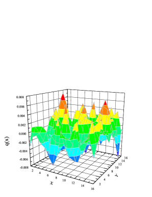
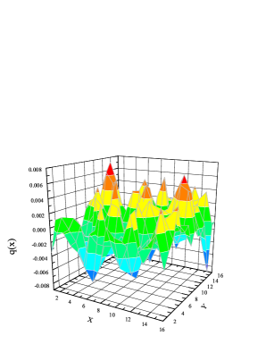
Figure 6: Topological charge density in a X-Y plane, by tracing $D_{\mathrm{ov}}$ with point sources (left) and SMP sources with $r_{\mathrm{min}}=4\sqrt{2}$ (right) on a $16^{4}$ configuration.

Firstly we calculated topological charge density exactly with point sources on a $16{}^{4}$ lattice and compared it to that using SMP sources with $r_{\mathrm{min}}=4\sqrt{2}$. The results of topological charge density in $X-Y$ plane with $t=1$ and $z=1$ are shown in Fig. 6. It’s obvious that there are quite similar peaks and valleys between the results by using point sources and SMP sources, which indicates the topological structure of the QCD vacuum is well reserved in the SMP method.

A series of gauge field configurations were then generated with different lattice spacing $a$ and different lattice volume. Topological charge density for each configuration was evaluated by SMP sources in different schemes, see Table 1, where the SMP scheme $P\left(m,m,m,m,\mathrm{mode}\right)$ is written as $\left(m,\mathrm{mode}\right)$ for short, and the lattice $L\left(n,n,n,n\right)$ is written as $n^{4}$. The number of point sources $N^{\mathrm{PT}}$ and SMP sources $N^{\mathrm{SMP}}$ are presented in Table 2, which are also the number of linear Eq. (7) that we had to solve by CG algorithm. It’s shown that the cost of calculating the topological charge density was sharply reduced for smaller $r_{\mathrm{min}}$ and larger lattices.

lattice	$a/\mathrm{fm}$	No. of config.	SMP scheme	$r_{\mathrm{min}}$
$12^{4}$	0.1	20	$\left(6,0\right)$$\left(6,1\right)$$\left(4,0\right)$$\left(4,1\right)$$\left(3,2\right)$$\left(3,0\right)$$\left(2,0\right)$	$2$, $2\sqrt{2}$, $3$, $3\sqrt{2}$, $4$, $4$, $6$
	0.133	20
$16^{4}$	0.1	20	$\left(8,0\right)$$\left(8,1\right)$$\left(4,2\right)$$\left(4,0\right)$$\left(4,1\right)$$\left(2,0\right)$	$2$, $2\sqrt{2}$, $4$, $4$, $4\sqrt{2}$, $8$
$24^{4}$	0.1	20	$\left(12,0\right)$$\left(12,1\right)$$\left(8,0\right)$$\left(8,1\right)$$\left(6,2\right)$$\left(6,0\right)$	$2$, $2\sqrt{2}$, $3$, $3\sqrt{2}$, $4$, $4$
$32^{4}$	0.1	20	$\left(16,0\right)$$\left(16,1\right)$$\left(8,2\right)$$\left(8,0\right)$	$2$, $2\sqrt{2}$, $4$, $4$

Table 1: Lattice setup and multi-probing scheme. Symmetric schemes $P\left(m,m,m,m,\mathrm{mode}\right)$ are written as $\left(m,\mathrm{mode}\right)$ for short.

lattice	$N^{\mathrm{SMP}}$	$N^{\mathrm{SMP}}/N^{\mathrm{PT}}$
$12^{4}$	192, 384, 972, 1944, 1536, 3072, 15552	$\frac{1}{1296}$, $\frac{1}{648}$, $\frac{1}{256}$, $\frac{1}{128}$, $\frac{1}{162}$, $\frac{1}{81}$, $\frac{1}{16}$
$16^{4}$	192, 384, 1536, 3072, 6144, 49152	$\frac{1}{4096}$, $\frac{1}{2048}$, $\frac{1}{512}$, $\frac{1}{256}$, $\frac{1}{128}$, $\frac{1}{16}$
$24^{4}$	192, 384, 972, 1944, 1536, 3072	$\frac{1}{20736}$, $\frac{1}{10368}$, $\frac{1}{4096}$, $\frac{1}{2048}$, $\frac{1}{2592}$, $\frac{1}{1296}$
$32^{4}$	192, 384, 1536, 3072	$\frac{1}{65536}$, $\frac{1}{32768}$, $\frac{1}{8192}$, $\frac{1}{4096}$

Table 2: Number of sources $N^{\mathrm{SMP}}$ required in different SMP scheme, and the ratio to $N^{\mathrm{PT}}$ referring to the number of point sources.

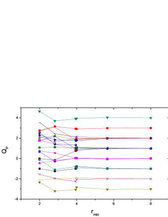
Figure 7: The series of $Q_{P}$ with different $r_{\mathrm{min}}$ for each configuration on $16^{4}$ lattice with $a=0.1\mathrm{fm}$. When $r_{\mathrm{min}}\geq 4$, $Q_{P}$ is very close to an integer value. Exact integer number of the topological charge were extracted since the systematic errors should be sharply suppressed as $r_{\mathrm{min}}$ increases.

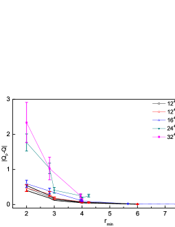
Figure 8: The average absolute error of $Q$ vs. $r_{\mathrm{min}}$ for all lattice setting. For $r_{\min}\geq 4$, the errors are small.

Since $Q_{P}$ (topological charge calculated in scheme $P$) should approach an integer and the deviation of $Q_{P}$ to its exact value will be always smaller than 0.1 as long as $r_{\mathrm{min}}$ is large enough, we extracted the topological charge $Q$ and absolute value of systematic error $\left|Q_{P}-Q\right|$ from the series of results with different $r_{\mathrm{min}}$ for each configuration, like an example in Fig. 7. The average errors are shown in Fig. 8, which decrease sharply as $r_{\mathrm{min}}$ increases. In general, the average absolute value of systematic error of $Q_{P}$ and its variance became small enough when $r_{\mathrm{min}}\geq 4$. One may notices that the error with $r_{\mathrm{min}}=3\sqrt{2}$ on $24^{4}$ lattice was larger than that of $r_{\mathrm{min}}=4$, which may come from more nearest neighbor terms (satisfying $\left|x-y\right|=r_{\mathrm{min}}$ in Eq. (17)) in $\mathrm{mode}=1$ case than $\mathrm{mode}=0$. There are 24 nearest neighbors for each site in the former mode while only 8 nearest neighbors in the latter mode.

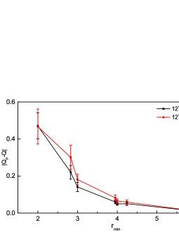
Figure 9: Comparing the average absolute error of $Q_{P}$ vs. $r_{\mathrm{min}}$ on $12^{4}$ lattice with different $a$. For the same $r_{\mathrm{min}}$, the finer lattice with smaller $a$ leads to smaller deviation of $Q$ to integer.

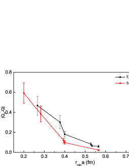
Figure 10: Comparing the average absolute error of $Q_{P}$ vs. physical distance $r_{\mathrm{min}}a$ on $V=\left(1.6\mathrm{fm}\right)^{4}$ lattice between different $a$. In physical unit, the errors are also smaller on finer lattice with the same volume.

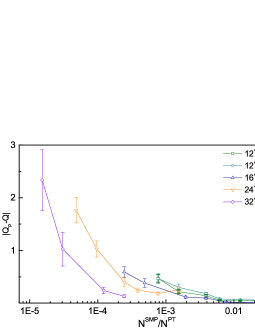
Figure 11: The errors versus the efficiency for all lattices. Larger lattice has higher efficiency.

Considering the same lattice with different lattice spacing $a$, Fig. 9 shows that finer lattice spacing $a$ leads to smaller errors. It could also be concluded from Fig. 10, which compares two lattices with the same physical volume. We finally present the errors versus efficiency in Fig. 11, which shows that for larger lattices, the calculation of trace by SMP method is more efficient to achieve sufficient accuracy.

$L$	$a/\mathrm{fm}$	$P$	$N^{\mathrm{SMP}}$	$\left\langle\left|Q_{P}-Q\right|\right\rangle$	$L$	$a/\mathrm{fm}$	$P$	$N^{\mathrm{SMP}}$	$\left\langle\left|Q_{P}-Q\right|\right\rangle$
$12^{4}$	$0.1$	$\left(6,0\right)$	192	$0.471\left(71\right)$	$16^{4}$	$0.1$	$\left(8,1\right)$	384	$0.384\left(79\right)$
		$\left(6,1\right)$	384	$0.220\left(37\right)$			$\left(4,2\right)$	1536	$0.0117\left(21\right)$
		$\left(4,0\right)$	972	$0.141\left(24\right)$			$\left(4,0\right)$	3072	$0.098\left(15\right)$
		$\left(4,1\right)$	1944	$0.051\left(10\right)$			$\left(4,1\right)$	6144	$0.022\left(3\right)$
		$\left(3,2\right)$	1536	$0.060\left(10\right)$			$\left(2,0\right)$	49152	$0.003\left(1\right)$
		$\left(3,0\right)$	3072	$0.049\left(7\right)$	$24^{4}$	$0.1$	$\left(12,0\right)$	192	$1.767\left(244\right)$
		$\left(2,0\right)$	15552	$0.010\left(2\right)$			$\left(12,1\right)$	384	$1.029\left(153\right)$
	$0.133$	$\left(6,0\right)$	192	$0.467\left(94\right)$			$\left(8,0\right)$	972	$0.406\left(81\right)$
		$\left(6,1\right)$	384	$0.301\left(65\right)$			$\left(8,1\right)$	1944	$0.253\left(41\right)$
		$\left(4,0\right)$	972	$0.181\left(29\right)$			$\left(6,2\right)$	1536	$0.250\left(36\right)$
		$\left(4,1\right)$	1944	$0.059\left(12\right)$			$\left(6,0\right)$	3072	$0.186\left(27\right)$
		$\left(3,2\right)$	1536	$0.082\left(16\right)$	$32^{4}$	$0.1$	$\left(16,0\right)$	192	$2.335\left(576\right)$
		$\left(3,0\right)$	3072	$0.065\left(11\right)$			$\left(16,1\right)$	384	$1.026\left(320\right)$
		$\left(2,0\right)$	15552	$0.010\left(2\right)$			$\left(8,2\right)$	1536	$0.242\left(63\right)$
$16^{4}$	$0.1$	$\left(8,0\right)$	192	$0.592\left(101\right)$			$\left(8,0\right)$	3072	$0.133\left(29\right)$

Table 3: The average of absolute systematic error $\left\langle\left|Q_{P}-Q\right|\right\rangle$ for different SMP scheme $P$.

All results of $\left\langle\left|Q_{P}-Q\right|\right\rangle$ are presented in Table 3. We can see for example, when $N^{\mathrm{SMP}}=3072$ the system error increases slowly as the lattice becomes larger. This could be understood since the number of non-zero off-diagonal elements in SMP sources is proportional to $N_{L}$, while $N^{\mathrm{SMP}}=3072$ is fixed. We can expect to apply this method on larger lattice with fixed $N^{\mathrm{SMP}}$, while $N_{\mathrm{PT}}$ is proportional to the lattice volumes $N_{L}$.

There is another method to calculate topological charge by calculating a few low modes of chiral Dirac operator, counting the number of zero modes and applying the index theorem. However, to estimate the topological charge density $q\left(x\right)$ one must calculate more low modes by applying low mode expansion [19]. We roughly compared the cost of SMP method and the calculation of low modes of the overlap operator on $12^{4}$ lattices. We considered $N^{\mathrm{SMP}}=3072$ with scheme $P\left(3,3,3,3,0\right)$, $r_{\mathrm{min}}=4$ in SMP method, and calculated the low modes of overlap operator by Arnordi algorithm with the number of low modes $N^{\mathrm{mode}}=100,\ 200$. The results showed that when $N^{\mathrm{mode}}=100$ , low modes calculation costs about $18\%$ less than SMP method, while $N^{\mathrm{mode}}=200$ it costs $28\%$ more than SMP method. However, since the number of zero modes is always an integer, the systematic errors of $q\left(x\right)$ from low mode expansion could hardly be estimated, while in SMP method the systematic errors of $Q$ and $q\left(x\right)$ are related. The comparison of $q\left(x\right)$ from SMP method and low mode expansion will be a interesting topic in our further studies.

4 Conclusion

Topological charge $Q$ and density $q\left(x\right)$ were calculated from the trace of overlap Dirac operator employing symmetric multi-probing sources on pure gauge configurations. The systematic error were suppressed when $r_{\mathrm{min}}$ increased as expected, due to the locality of overlap Dirac operator. Thus the estimated topological charge were close enough to an integer while $r_{\mathrm{min}}\geq 4$ or $r_{\mathrm{min}}\geq 4\sqrt{2}$, in which case the number of required sources $N^{\mathrm{SMP}}=12r_{\mathrm{min}}^{4}\ \mathrm{or}\ 24r_{\mathrm{min}}^{4}$ comparing to that with point sources $N^{\mathrm{PT}}=12N_{L}$. Notice that $N^{\mathrm{SMP}}$ only depends on the chosen $r_{\mathrm{min}}$ and is independent of $N_{L}$. Furthermore, we found that the introduced systematic errors of SMP method for the same $r_{\mathrm{min}}$ grew slowly with larger $N_{L}$, which meant the time to estimate the trace is much less dependent on the lattice volumes $N_{L}$. Thus it will be much more economical to employ SMP method on larger lattices. Since the introduced error of the trace comes from the off-diagonal elements of the matrix, we can expect better performance of this method by employing some techniques to suppress the off-diagonal elements of $D_{\mathrm{ov}}$ in future work. This method is also supposed to work well when dealing with ultra-local matrix such as Wilson Dirac operator $D_{\mathrm{W}}$, and $\mathrm{Tr}D_{\mathrm{W}}^{-1}$ is very important and quite expensive to determinate exactly in lattice QCD.

As mentioned above, we developed symmetric scheme with 3 modes in coloring algorithm and evaluated the topological charge with SMP method. Results of average absolute systematic error are presented, as well as the efficiency of SMP method compared to point source method. Potential applications of SMP method are expected in calculating the trace of the inverse of any large sparse matrix with locality.

5 References

References

- [1] E. Witten. Current algebra theorems for the U(1) "Goldstone boson". Nucl. Phys. B, 156(2):269–283, 1979.
- [2] G. Veneziano. U(1) without instantons. Nucl. Phys. B, 159(1-2):213–224, 1979.
- [3] M. Lüscher. Topology of lattice gauge fields. Communications in Mathematical Physics, 85(1):39–48, 1982. 10.1007/BF02029132.
- [4] Ferenc Niedermayer. Exact chiral symmetry, topological charge and related topics. Nucl. Phys. Proc. Suppl., 73:105–119, 1999.
- [5] Michael F Atiyah and Isadore M Singer. The index of elliptic operators: Iv. Annals of Mathematics, pages 119–138, 1971.
- [6] Herbert Neuberger. Exactly massless quarks on the lattice. Phys. Lett. B, 417:141–144, 1998.
- [7] Herbert Neuberger. More about exactly massless quarks on the lattice. Phys. Lett. B, 427:353–355, 1998.
- [8] EI Zolotarev. Application of elliptic functions to questions of functions deviating least and most from zero. Zap. Imp. Akad. Nauk. St. Petersburg, 30(5):1–59, 1877.
- [9] Y. Chen, S. J. Dong, T. Draper, I. Horváth, F. X. Lee, K. F. Liu, N. Mathur, and J. B. Zhang. Chiral logarithms in quenched qcd. Phys. Rev. D, 70:034502, Aug 2004.
- [10] Pilar Hernandez, Karl Jansen, and Martin Luscher. Locality properties of Neuberger’s lattice Dirac operator. Nucl. Phys. B, 552:363–378, 1999.
- [11] C. Bekas, E. Kokiopoulou, and Y. Saad. An estimator for the diagonal of a matrix. Applied Numerical Mathematics, 57(11-12):1214–1229, 2007.
- [12] Jok M. Tang and Yousef Saad. A probing method for computing the diagonal of a matrix inverse. Numerical Linear Algebra with Applications, 19(3):485–501, 2012.
- [13] Andreas Stathopoulos, Jesse Laeuchli, and Kostas Orginos. Hierarchical probing for estimating the trace of the matrix inverse on toroidal lattices. SIAM Journal on Scientific Computing, 35(5):S299–S322, 2013.
- [14] Eric Endress, Carlos Pena, and Karthee Sivalingam. Variance reduction with practical all-to-all lattice propagators. Comput. Phys. Commun., 195:35–48, 2015.
- [15] Eric Endress and Carlos Pena. Exploring the role of the charm quark in the I=1/2 rule. Phys. Rev. D, 90:094504, 2014.
- [16] E. M. Ilgenfritz, K. Koller, Y. Koma, G. Schierholz, T. Streuer, and V. Weinberg. Exploring the structure of the quenched QCD vacuum with overlap fermions. Phys. Rev. D, 76:034506, 2007.
- [17] Yoshiaki Koma, Ernst-Michael Ilgenfritz, Karl Koller, Miho Koma, Gerrit Schierholz, Thomas Streuer, and Volker Weinberg. Momentum dependence of the topological susceptibility with overlap fermions. PoS, LATTICE2010:278, 2010.
- [18] A. Ali Khan et al. Chiral properties of domain wall quarks in quenched QCD. Phys. Rev. D, 63:114504, 2001.
- [19] Ivan Horváth, Shao-Jing Dong, Terrence Draper, Frank X Lee, KF Liu, Harry B Thacker, and Jian-Bo Zhang. Local structure of topological charge fluctuations in qcd. Phys. Rev. D, 67(1):011501, 2003.