Emergence of photo-induced multiple topological phases on square-octagon lattice

Abstract

In this study, a tight-binding model on square-octagon lattice with nearest-neighbour and next-nearest-neighbour hoppings is considered. The system is topologically trivial although it exhibits quadratic band-touching points in its band-structure. It is shown that the system drives towards topologically non-trivial phases as soon as it is exposed to monochromatic circularly polarized light. Multiple topological phases are found to emerge with the variation of amplitude of light. An effective time-independent Hamiltonian of the system is obtained following the Floquet-Bloch formulation. Quasi-energy band-structures along with definite values of Chern numbers for respective bands are obtained. Characterization of topological phases are made in terms of band structure and Chern numbers. In addition, Hall conductance and topologically protected chiral edge states are obtained to explain the topological properties. Density of states is obtained in every case. The system undergoes a series of topological phase transitions among various topological phases upon variations of both amplitude of light and hopping strengths. It exhibits Chern insulating and Chern semimetallic phases depending on the values of lattice filling.

today

I Introduction

Topological phases of matter have become the centre of attraction among the researchers in recent years Kane2 . A considerable portion of these investigations includes the study of topological insulators (TI) or quantum spin Hall (QSH) phase, Chern insulators or quantum anomalous Hall phase, topological Dirac or Weyl semimetals, to name a few. Depending on the nature of time reversal symmetry (TRS), particle-hole symmetry and chiral symmetry of the systems, ten classes of topological insulators have been proposed Ryu . A transition from either trivial band-insulators or semimetals to non-trivial topological phases traditionally occurs in two different ways. Either it is driven by artificial gauge-field in case of Chern insulators, where each energy band is characterized by the integral Chern number ($C$) TKNN , or spin-orbit coupling (SOC) in case of QSH effect, where the resulting system is characterized by a non-trivial $Z_{2}$ invariant Kane2 . Haldane first demonstrated the emergence of Chern insulating (CI) phase in a two-band model on graphene by introducing an artificial phase coupled with next-nearest neighbour hopping, which breaks TRS Haldane . On the other hand, QSH was also initially proposed on graphene, but with intrinsic SOC instead, providing a net TRS Kane1 .

Besides those two ways, another route for driving the system into non-trivial topological phases has been established by a series of recent investigations. That particular state of matter is known as Floquet topological insulator (FTI) which is obtained by perturbing the system with a coherent periodic photo-irradiations Oka ; Inoue1 . Topological classification of periodically driven quantum systems has been formulated Kitagawa . So, in order to study the FTI phase in a tight-binding system, one has to develop an appropriate Floquet-Bloch theory on it. A section of investigations is now devoted to find the existence of FTI phase within the systems those were otherwise declared as topologically trivial. These kind of investigations may help the experimentalists to develop suitable techniques for probing the existence of novel topological phases within the materials. In addition, associated topological phase transitions can also be demonstrated by modulating the appropriate parameters of the irradiation Inoue2 .

Emergence of quasi-continuous edge-states on the surface of the material is one of the most significant evidence of any kind of TI. These topologically protected edge states are obtained for finite system in open boundary condition (OBC) and in general they tend to obey the ‘bulk-boundary correspondence’ rule Hatsugai1 ; Hatsugai2 . Following the successful achievement in the field of conventional electronic TI’s, their bosonic analogs, namely topological magnon insulators have also drawn attention in more recent years Mook ; Owerre3 ; Kim .

Existence of FTI phase was also predicted in graphene for the first time. Since then there have been several studies on Floquet topological phase on honeycomb lattice Mitra1 ; Kundu ; Rigol ; Torres ; Li in addition to other two-band systems Saha ; Galitski ; Ezawa ; Platero . It has been shown that the effect of periodically driven circularly polarized light leads to a non-trivial mass term similar to that found in Haldane model Moessner . This mass term now becomes a function of both the intensity and the state of polarization of light. So, detection of a particular non-trivial topological phase requires appropriate value of intensity and definite state of polarization of the light. In addition to the honeycomb lattice, effect of photo-irradiation is studied before on three-band tight-binding models formulated on kagomé Fiete1 and Lieb Ren lattices. Again, in these tight-binding models, photo-irradiation opens up gaps in the otherwise gapless spectrum and the resulting energy-bands are found to emerge simultaneously with non-zero Chern numbers. Interestingly, in two-dimensional Floquet systems, evidence of chiral edge states is found even though the Chern numbers of the respective bulk bands are zero, which indicates the violation of ‘bulk-boundary correspondence’ rule for that particular system Kitagawa ; Rudner . Therefore, determination of both $C$ for the bulk-bands and edge states between the respective bands are necessary to confirm the topological phases. Recently, the bosonic counterpart of FTI phase has been formulated in magnetic systems Owerre1 .

In this work, we pay attention to the four-band tight-binding model on square-octagon lattice. It has been reported that this model exhibits $Z_{2}$ band-insulating and CI phases in the presence of spin-orbit coupling Fiete2 and external magnetic flux Pal ; Gong , respectively. Topological phase transition (TPT) driven by SOC and exchange field are also found on this lattice Yang . Outcome of those studies based on square-octagon lattice along with the emergence of photoinduced topological phases on kagomé and Lieb lattices motivate us to search the FTI phase on this particular lattice.

The intrinsic tight-binding model on square-octagon lattice has an interesting band-structure which includes a pair of flat band and five different band-touching points. The coherent photo-irradiation perturbs the band structure in such a manner that either true or pseudo band-gaps appear depending on the value of its amplitude. System undergoes a series of topological phase transition with the variation of amplitude, where successive band-touching and gap-opening processes occur at the transition points separating the different topological phases. As a result, multiple topological phases are found to emerge in the parameter space, which can be categorized as either Chern semimetallic (CSM) or CI phases depending on the nature of band-gap. CSM (CI) phase appears in case of pseudo (true) band-gap. Rapid variation of topological phases with respect to the amplitude of irradiation is observed which is not reported before for the cases of honeycomb, kagomé and Lieb lattices. Chiral edge states are found to appear in finite system according to the ‘bulk-boundary correspondence’ rule which confirms the existence of non-trivial topological phases.

The plan of the paper is as follows. In section II, square-octagon lattice is described and the tight-binding Hamiltonian is formulated. Outline of Floquet theory and development of Floquet-Bloch effective Hamiltonian are presented in section III. Detailed characterization of various topological phases and transition among them along with explanations are provided in section IV. Section V contains discussion on the theme of this work.

II Model Hamiltonian and Band Structure

We consider a two-dimensional square-octagon lattice model consisting of two elementary plaquettes: square and octagon as shown in Fig 1. The same lattice is noted before as 1/5-depleted square lattice Ueda and Archimedean lattice T11 Yu in the context of investigations of several other properties based on it. The coordination number of this non-Bravais lattice is three which is similar to that of honeycomb lattice, another non-Bravais one. However, this lattice can be considered as composed of four interpenetrating square sub-lattices each of which is formed by lattice points those are drawn by four different colours in Fig 1. The tight binding Hamiltonian considering nearest-neighbour (NN) and next-nearest-neighbour (NNN) interactions can be written as

$$H\!\! = \!\!\!-\!\!\!\!\sum_{(m,n)}\!\!\bigg{[}t_{1}\!\sum_{\langle ij\rangle}c_{m,n,i}^{\dagger}\,c_{m,n,j}\!+\!t_{2}\!\sum_{\langle\langle ij\rangle\rangle}c_{m,n,i}^{\dagger}\,c_{m,n,j}\!+\!H.c\bigg{]}.$$

\psfrag{j}{\text{\tiny{\bf$\delta_{5}$}}}\psfrag{b}{\text{\tiny{\bf$\delta_{6}$}}}\psfrag{c}{\text{\tiny{\bf$\delta_{1}$}}}\psfrag{h}{\text{\tiny{\bf$\delta_{2}$}}}\psfrag{d}{\text{\tiny{$\Gamma$}}}\psfrag{e}{\text{\tiny{K}}}\psfrag{f}{\text{\tiny{M}}}\psfrag{x}{\text{\scriptsize{$x$}}}\psfrag{y}{\text{\scriptsize{$y$}}}\psfrag{E}{\text{\tiny{\bf$\delta_{3}$}}}\psfrag{F}{\text{\tiny{\bf$\delta_{4}$}}}\psfrag{(a)}{\text{{(a)}}}\psfrag{(b)}{\text{\scriptsize{$(b)$}}}\includegraphics[width=176.407pt,height=176.407pt]{Fig1a.eps}

\psfrag{j}{\text{\tiny{\bf$\delta_{5}$}}}\psfrag{b}{\text{\tiny{\bf$\delta_{6}$}}}\psfrag{c}{\text{\tiny{\bf$\delta_{1}$}}}\psfrag{h}{\text{\tiny{\bf$\delta_{2}$}}}\psfrag{d}{\text{\tiny{$\Gamma$}}}\psfrag{e}{\text{\tiny{K}}}\psfrag{f}{\text{\tiny{M}}}\psfrag{x}{\text{\scriptsize{$x$}}}\psfrag{y}{\text{\scriptsize{$y$}}}\psfrag{E}{\text{\tiny{\bf$\delta_{3}$}}}\psfrag{F}{\text{\tiny{\bf$\delta_{4}$}}}\psfrag{(a)}{\text{{(a)}}}\psfrag{(b)}{\text{\scriptsize{$(b)$}}}\includegraphics[width=51.21504pt]{Fig1b.eps}

Figure 1: (Color online) (a) The geometry of square-octagon lattice. $A,B,C,D$ denote four different sites in the unit cell which is shown by large square (pink dashed lines). Strength of NN hopping along sides (black solid lines) of small square is $t_{1}$. Strength of NNN hopping along diagonals (red dotted lines) of small square is $t_{2}$. $\boldsymbol{\delta}_{1},\boldsymbol{\delta}_{2},\boldsymbol{\delta}_{3},\boldsymbol{\delta}_{4}$ are the NN vectors and $\boldsymbol{\delta}_{5},\boldsymbol{\delta}_{6}$ are the NNN vectors. (b) The first Brillouin zone of the lattice. High-symmetry points $\Gamma$, K and M have been marked.

The first summation $(m,n)$ runs over the unit cell indices, while the second summations $\langle\cdot\rangle$ and $\langle\langle\cdot\rangle\rangle$ run over NN and NNN pairs, respectively. $c_{m,n,i}^{\dagger}\,(c_{m,n,i})$ is the creation (annihilation) operator for an electron at the $i$-th site of the $(m,n)$-th unit cell. $t_{1}$ is the strength of NN hopping while $t_{2}$ is that of NNN hopping those occur along the diagonals of each square plaquette. By setting the distance between NN points to be unity, four NN vectors are defined as $\boldsymbol{\delta}_{1}=1/\sqrt{2}\left(1,-1\right),\;\boldsymbol{\delta}_{2}=1/\sqrt{2}\left(1,1\right),\;\boldsymbol{\delta}_{3}=\left(0,1\right)$, and $\boldsymbol{\delta}_{4}=\left(1,0\right)$. Similarly, two NNN vectors are $\boldsymbol{\delta}_{5}=\sqrt{2}\left(0,1\right)$, and $\boldsymbol{\delta}_{6}=\sqrt{2}\left(1,0\right)$. The lattice translation vectors are $\boldsymbol{a}_{1}=\left(1+\sqrt{2},0\right)$ and $\boldsymbol{a}_{2}=\left(0,1+\sqrt{2}\right)$. Position of each unit cell is defined by $\boldsymbol{R}\left(m,n\right)=m\boldsymbol{a}_{1}+n\boldsymbol{a}_{2}$. We set $t_{1}=1.0$ throughout the article.

Fourier transforming to the momentum space, the Hamiltonian becomes $H=-\sum_{\textbf{k}}\psi_{\textbf{k}}^{\dagger}\,H(\textbf{k})\,\psi_{\textbf{k}}$, where

$$H(\textbf{k})\!=\!\left(\begin{matrix}0&t_{1}&t_{1}e^{ik_{2}}\!+\!t_{2}&t_{1}\\ t_{1}&0&t_{1}&t_{1}e^{-ik_{1}}\!+\!t_{2}\\ t_{1}e^{-ik_{2}}\!+\!t_{2}&t_{1}&0&t_{1}\\ t_{1}&t_{1}e^{ik_{1}}\!+\!t_{2}&t_{1}&0\end{matrix}\right)$$ (2)

with $\psi_{\textbf{k}}={\left(A_{\textbf{k}},B_{\textbf{k}},C_{\textbf{k}},D_{\textbf{k}}\right)}^{T}$, where $\alpha_{\textbf{k}}$ with $\alpha=A,B,C,D$ are the electron annihilation operators on the four basis sites in the square unit cell, $k_{1}=\boldsymbol{k}\cdot\boldsymbol{a}_{1}$ and $k_{2}=\boldsymbol{k}\cdot\boldsymbol{a}_{2}$.

\psfrag{E}{\text{\scriptsize{Energy}}}\psfrag{K1}{$k_{1}$}\psfrag{K2}{$k_{2}$}\psfrag{$3$}{$\pi$}\psfrag{c0}{\text{\tiny{\bf{$C=0$}}}}\psfrag{c2}{\text{\tiny{\bf{$C=2$}}}}\psfrag{c-2}{\text{\tiny{\bf{$C=-2$}}}}\psfrag{c1}{\text{\tiny{\bf{$C=1$}}}}\psfrag{c-1}{\text{\tiny{\bf{$C=-1$}}}}\psfrag{p}{\text{\tiny{$E_{1}$}}}\psfrag{q}{\text{\tiny{$E_{2}$}}}\psfrag{r}{\text{\tiny{$E_{3}$}}}\psfrag{s}{\text{\tiny{$E_{4}$}}}\includegraphics[width=113.81102pt,height=142.26378pt,trim=56.9055pt 19.91684pt 91.04872pt 14.22636pt]{Fig2a.eps}

\psfrag{E}{\text{\scriptsize{Energy}}}\psfrag{K1}{$k_{1}$}\psfrag{K2}{$k_{2}$}\psfrag{$3$}{$\pi$}\psfrag{c0}{\text{\tiny{\bf{$C=0$}}}}\psfrag{c2}{\text{\tiny{\bf{$C=2$}}}}\psfrag{c-2}{\text{\tiny{\bf{$C=-2$}}}}\psfrag{c1}{\text{\tiny{\bf{$C=1$}}}}\psfrag{c-1}{\text{\tiny{\bf{$C=-1$}}}}\psfrag{p}{\text{\tiny{$E_{1}$}}}\psfrag{q}{\text{\tiny{$E_{2}$}}}\psfrag{r}{\text{\tiny{$E_{3}$}}}\psfrag{s}{\text{\tiny{$E_{4}$}}}\includegraphics[width=113.81102pt,height=142.26378pt,trim=56.9055pt 14.22636pt 91.04872pt 14.22636pt]{Fig2b.eps}

\psfrag{E}{\text{\scriptsize{Energy}}}\psfrag{K1}{$k_{1}$}\psfrag{K2}{$k_{2}$}\psfrag{$3$}{$\pi$}\psfrag{c0}{\text{\tiny{\bf{$C=0$}}}}\psfrag{c2}{\text{\tiny{\bf{$C=2$}}}}\psfrag{c-2}{\text{\tiny{\bf{$C=-2$}}}}\psfrag{c1}{\text{\tiny{\bf{$C=1$}}}}\psfrag{c-1}{\text{\tiny{\bf{$C=-1$}}}}\psfrag{p}{\text{\tiny{$E_{1}$}}}\psfrag{q}{\text{\tiny{$E_{2}$}}}\psfrag{r}{\text{\tiny{$E_{3}$}}}\psfrag{s}{\text{\tiny{$E_{4}$}}}\includegraphics[width=113.81102pt,height=142.26378pt,trim=56.9055pt 14.22636pt 91.04872pt 14.22636pt]{Fig2c.eps}

\psfrag{E}{\text{\scriptsize{Energy}}}\psfrag{K1}{$k_{1}$}\psfrag{K2}{$k_{2}$}\psfrag{$3$}{$\pi$}\psfrag{c0}{\text{\tiny{\bf{$C=0$}}}}\psfrag{c2}{\text{\tiny{\bf{$C=2$}}}}\psfrag{c-2}{\text{\tiny{\bf{$C=-2$}}}}\psfrag{c1}{\text{\tiny{\bf{$C=1$}}}}\psfrag{c-1}{\text{\tiny{\bf{$C=-1$}}}}\psfrag{p}{\text{\tiny{$E_{1}$}}}\psfrag{q}{\text{\tiny{$E_{2}$}}}\psfrag{r}{\text{\tiny{$E_{3}$}}}\psfrag{s}{\text{\tiny{$E_{4}$}}}\includegraphics[width=113.81102pt,height=142.26378pt,trim=56.9055pt 19.91684pt 99.58464pt 14.22636pt]{Fig2d.eps}

Figure 2: (Color online) (a) Band diagram of tight-binding square-octagon lattice without any external perturbation when $t_{2}=1.0$. Floquet-Bloch band diagram in the presence of circularly polarized light for $t_{2}=1.0$ $\Omega=7,A_{0}=0.8$ (b), $t_{2}=1.0,\Omega=10,A_{0}=2.1$ (c), $t_{2}=0.6,\Omega=10,A_{0}=2.7$ (d).

Diagonilizing the Hamiltonian we get two flat bands, ($E_{1},E_{3}$) and two dispersive bands with energies $E_{2,4}(\textbf{k})=1\pm\sqrt{5+2\cos{k_{1}}+2\cos{k_{2}}}$, as shown in Fig 2 (a), when $t_{2}=1.0$. The bands are denoted as $E_{1},E_{2},E_{3}$ and $E_{4}$ in the ascending order of energy. We note that, the lower two bands touch at the $\Gamma$ point while the energy bands $E_{2}(\textbf{k})$ and $E_{3}$ touch at four M points of the first Brillouin zone (BZ). All these are quadratic band touching points since the energy of the lower dispersive band, $E_{2}(\textbf{k})$, is found to become proportional to the square of the wave-vectors when expanded in the vicinity of those points as shown below.

$${E_{2}(k_{1},k_{2})|}_{k_{1},k_{2}\to 0} =-2+\frac{{k_{1}}^{2}+{k_{2}}^{2}}{6},$$ (3)

$${E_{2}(k_{1},k_{2})|}_{k_{1},k_{2}\to\pi} =-\frac{{(k_{1}-\pi)}^{2}}{2}-\frac{{(k_{2}-\pi)}^{2}}{2}.$$

The model without NNN hopping has been studied before in the absence of circularly polarized light. In this case, Dirac cones are found to appear at $\Gamma$ and M points when the intra- and inter-square-plaquette NN hopping strengths are different. Ueda .

\psfrag{DOS}{\text{\tiny{DOS}}}\psfrag{E}{\text{\scriptsize{Energy}}}\psfrag{G}{$\Gamma$}\psfrag{c0}{\text{\tiny{\bf{$C=0$}}}}\psfrag{c2}{\text{\tiny{\bf{$C=2$}}}}\psfrag{c-2}{\text{\tiny{\bf{$C=-2$}}}}\psfrag{c1}{\text{\tiny{\bf{$C=1$}}}}\psfrag{c-1}{\text{\tiny{\bf{$C=-1$}}}}\includegraphics[width=426.79134pt]{Fig3.eps}

Figure 3: (Color online) Floquet-Bloch band diagram of the tight-binding square-octagon lattice along the high-symmetry points of BZ. (a) Without any external perturbation for $t_{2}=1.0$. (b) In the presence of circularly polarized light when $t_{2}=1.0,\Omega=7,A_{0}=0.8$. System clearly exhibits the CI phase for 1/4 filling and CSM phase for 1/2 filling as true band gap only exists between the two lower bands. (c) When $t_{2}=1.0,\Omega=10,A_{0}=2.1$, the system exhibits the CI phase for both 1/2 and 3/4 fillings. True band gap exists between all the bands. (d) When $t_{2}=0.6,\Omega=10,A_{0}=2.7$, CI and CSM phases appear for 1/2 and 3/4 fillings, respectively. Chern numbers of the respective energy-bands are noted. Density of states are also shown in the right panels. Horizontal dashed lines are drawn for the determination of true and pseudo band-gaps.

III Derivation of Effective Hamiltonian by Floquet-Bloch Theory

In order to apply the Floquet-Bloch theory, the system is exposed to periodically driven monochromatic laser light which couples the momentum with the vector potential of the incident field $\textbf{A}\!=\!\textbf{A}_{0}\left[\sin(\Omega t),\cos(\Omega t)\right]$ through the substitution $\textbf{k}\rightarrow\textbf{k}+\textbf{A}(t)$. $\textbf{A}_{0}$ and $\Omega$ are respectively amplitude and frequency of the laser light. Values of the relevant constants are assumed to be unity, so, $\hbar=1,e=1,c=1$. Therefore, the time-dependent Hamiltonian looks like,

$$H(\textbf{k},t) =-t_{1}\sum_{\textbf{k}}\left[{A_{\textbf{k}}}^{\dagger}B_{\textbf{k}}e^{-i\textbf{A}(t)\cdot\mathbf{\delta_{2}}}+{A_{\textbf{k}}}^{\dagger}D_{\textbf{k}}e^{i\textbf{A}(t)\cdot\mathbf{\delta_{1}}}\right.$$ (4)

$$+\left.{B_{\textbf{k}}}^{\dagger}D_{\textbf{k}}e^{-i\textbf{k}\cdot\textbf{R}\left(1,0\right)}e^{-i\textbf{A}(t)\cdot\mathbf{\delta_{4}}}+{B_{\textbf{k}}}^{\dagger}C_{\textbf{k}}e^{i\textbf{A}(t)\cdot\mathbf{\delta_{1}}}\right.$$

$$+\left.{A_{\textbf{k}}}^{\dagger}C_{\textbf{k}}e^{i\textbf{k}\cdot\textbf{R}\left(0,1\right)}e^{i\textbf{A}(t)\cdot\mathbf{\delta_{3}}}+{C_{\textbf{k}}}^{\dagger}D_{\textbf{k}}e^{i\textbf{A}(t)\cdot\mathbf{\delta_{2}}}\right]$$

$$-t_{2}\sum_{\textbf{k}}\left[{A_{\textbf{k}}}^{\dagger}C_{\textbf{k}}e^{-i\textbf{A}(t)\cdot\mathbf{\delta_{5}}}+{B_{\textbf{k}}}^{\dagger}D_{\textbf{k}}e^{i\textbf{A}(t)\cdot\mathbf{\delta_{6}}}\right].$$

Now, the Hamiltonian becomes periodic with time period $T=2\pi/\Omega$ like $H(\textbf{k},t)=H(\textbf{k},t+T)$ because of the periodicity of ${\textbf{A}}(t)$ and monochromaticity of the laser light. This time-periodicity allows one to map the time-dependent problem into an effective time-independent problem by virtue of Floquet theory Floquet as described below. By performing the Fourier transform in the time space, the periodic Hamiltonian can be expressed as $H(\textbf{k},t)=\sum_{p=-\infty}^{\infty}e^{ip\Omega t}H_{p}\left(\textbf{k}\right)$, where $H_{p}\left(\textbf{k}\right)=\frac{1}{T}\int_{0}^{T}e^{-ip\Omega t}H(\textbf{k},t)\,dt=H_{-p}^{\dagger}\left(\textbf{k}\right)$ is the $p$-th order Fourier component. By considering the time-dependent Schrödinger equation for the system,

$$i\hbar\,\frac{d}{dt}\ket{\psi(\textbf{k},t)}=H(\textbf{k},t)\,\psi(\textbf{k},t),$$ (5)

one may have the solution for the $\alpha$-th band as

$$\psi_{\alpha}(\textbf{k},t)=e^{i\epsilon_{\alpha}(\textbf{k})t}\phi_{\alpha}(\textbf{k},t),$$ (6)

where $\phi_{\alpha}(\textbf{k},t)$ and $\epsilon_{\alpha}(\textbf{k})$ are known as the time-periodic Floquet-Bloch wave function and Floquet quasi-energy of that band, respectively. Floquet-Bloch wave function can be expressed in the Fourier space as $\phi_{\alpha}(\textbf{k},t)=\sum_{p=-\infty}^{\infty}e^{ip\Omega t}\phi_{\alpha,p}\left(\textbf{k}\right)$. Temporal periodicity of the Hamiltonian leads to the appearance of periodicity of the quasi-energies in the frequency space with period $\Omega$, which, on the other hand, gives rise to the existence of quasi-energy BZ bounded within the limits $-\Omega/2<\epsilon<\Omega/2$. This result is similar to the appearance of periodicity for the energy of Bloch electron in the momentum space.

By using Eqs (5, 6) and defining the Floquet operator as $H_{F}(\textbf{k},t)=H(\textbf{k},t)-i\partial_{t}$, the following eigenvalue equation for the Floquet-Bloch wave function is obtained.

$$H_{F}(\textbf{k},t)\ket{\phi_{\alpha}(\textbf{k},t)}=\epsilon_{\alpha}(\textbf{k})\ket{\phi_{\alpha}(\textbf{k},t)}.$$ (7)

Solution of this equation in the Fourier space leads to a time-independent Floquet eigenvalue problem,

$$\sum_{q}\left[H_{p-q}(\textbf{k})+q\,\Omega\,\delta_{p,q}\right]\ket{\phi_{\alpha,q}(\textbf{k})}=\epsilon_{\alpha}(\textbf{k})\ket{\phi_{\alpha,p}(\textbf{k})}.$$ (8)

Floquet theory finally leads to a set of infinite-dimensional coupled equations since both the Floquet numbers, $p$ and $q$ may assume any integral values in between $-\infty$ and $+\infty$. But, if the frequency of the incident light is greater than that of corresponding band-width of the system, the Floquet sub-bands become decoupled. In this limit, one can apply Floquet-Magnus expansion Polkovnikov to describe the system in terms of an effective Hamiltonian, $H_{\rm eff}$, which can be written as $H_{\rm eff}=\sum_{i}\frac{H_{\rm eff}^{i}}{{\Omega}^{i}}$ where $H_{\rm eff}^{0}=H^{0}$ and $H_{\rm eff}^{1}=\sum_{p=1}^{\infty}\frac{1}{p}\left[H_{p},H_{-p}\right]$. $H_{p}$ is the $p$-th order Fourier component. Ignoring the higher order components ($|p|\geq 2$) for high frequency, $H_{\rm eff}$ is finally given by

$$H_{\rm eff}=H_{0}+\frac{1}{\Omega}\left[H_{1},H_{-1}\right].$$ (9)

Throughout this investigation, frequency of the light is kept greater than that of the band-width of the undriven system, i.e., the system is always kept in the off-resonant regime. Although the electrons cannot be excited by direct absorption of this kind of irradiation, but instead the light is capable to modify the single-electron bands through virtual photon-absorption processes Kitagawa2 ; Ezawa . In Eq 9, $H_{0}$ describes the system where no photon exchange takes place, while $H_{1}$ ($H_{-1}$) takes into account the emission (absorption) of one virtual photon.

After obtaining the expression of $H_{0},H_{1}$ and $H_{-1}$, the effective time-independent Hamiltonian $H_{\rm eff}$ for the system is written as $H_{\rm eff}=-\sum_{\textbf{k}}\psi_{\textbf{k}}^{\dagger}H_{\rm eff}(\textbf{k})\psi_{\textbf{k}}$. The derivation of $H_{\rm eff}$ is available in Appendix A. The diagonal elements of $H_{\rm eff}(\textbf{k})$ are zero. The off-diagonal upper-triangular elements of $H_{\rm eff}(\textbf{k})$ are written below.

$$H_{\rm eff}^{12}(\textbf{k}) =J_{0}(A_{0})t_{1}-4iPt_{1}t_{2}+2iQt_{1}^{2}(e^{ik_{1}}+e^{ik_{2}}),$$

$$H_{\rm eff}^{13}(\textbf{k}) =J_{0}(\sqrt{2}A_{0})t_{2}+J_{0}(A_{0})t_{1}e^{ik_{2}},$$

$$H_{\rm eff}^{14}(\textbf{k}) =J_{0}(A_{0})t_{1}+4iPt_{1}t_{2}-2iQt_{1}^{2}(e^{-ik_{1}}+e^{ik_{2}}),$$

$$H_{\rm eff}^{23}(\textbf{k}) =J_{0}(A_{0})t_{1}-4iPt_{1}t_{2}+2iQt_{1}^{2}(e^{-ik_{1}}+e^{ik_{2}}),$$

$$H_{\rm eff}^{24}(\textbf{k}) =J_{0}(\sqrt{2}A_{0})t_{2}+J_{0}(A_{0})t_{1}e^{-ik_{1}},$$

$$H_{\rm eff}^{34}(\textbf{k}) =J_{0}(A_{0})t_{1}-4iPt_{1}t_{2}+2iQt_{1}^{2}(e^{-ik_{1}}+e^{-ik_{2}}).$$

$H_{\rm eff}^{pq}(\textbf{k})$ are the elements of $p$-th row and $q$-th column of the $4\times 4$ Hamiltonian, $H_{\rm eff}(\textbf{k})$, where the constants $P$ and $Q$ are given by

$$P =J_{1}(A_{0})J_{1}(\sqrt{2}A_{0})\sin(\pi/4)/\Omega,$$ (10)

$$Q ={J_{1}}^{2}(A_{0})\sin(\pi/4)/\Omega.$$

Here $J_{n}(x)$ is the $n$-th order Bessel function given by $J_{n}(x)=\frac{1}{2\pi}\int_{0}^{2\pi}e^{-i(n\tau-x\sin(\tau)}d\tau$.

It is evident that the circularly polarized light breaks the TRS of the undriven system since $H_{\rm eff}(\textbf{k})\neq H_{\rm eff}^{\ast}(-\textbf{k})$. As soon as the periodic drive is turned on, i.e., $A_{0}$ becomes non-zero, gaps appear in the band structure. At the same time, the system becomes topologically nontrivial in a sense that every band emerges with a definite value of Chern number. Band diagrams obtained by numerically diagonalizing the effective Hamiltonian $H_{\rm eff}(\textbf{k})$ are shown in Fig 2 (b), (c) and (d) for few particular sets of parameter, $t_{2},A_{0}$ and $\Omega$. The Chern numbers of respective bands are also noted. The sets of parameters are chosen in such a way that distribution of $C$ for the four energy bands are different. In those figures, ‘Energy’ actually means the quasi-energies of the effective Hamiltonian since $A_{0}$ is non-zero. With the increase of $A_{0}$ beyond zero, both the flat-bands begin to become dispersive. At the same time, the remaining two bands get modified in such a fashion that a series of topological phase transitions occur, which will be described in detail in the next section. Dispersion relations along the path connecting the high-symmetry points of BZ are shown in Fig 3 (b), (c) and (d).

The system exhibits true and pseudo gap in the band diagram for different parameter regimes and the corresponding topological phases are noted as CI and CSMLieb , respectively, depending on the lattice fillings. True and pseudo band-gaps are defined in the following way. If $E_{m}(\textbf{k})\neq E_{n}(\textbf{k}^{\prime})$ for all $m\neq n$ and k, $\textbf{k}^{\prime}$, then true gap exists between $m$ and $n$-th energy bands. The gap is marked pseudo when $E_{m}(\textbf{k})\neq E_{n}(\textbf{k})$ for all $m\neq n$ and k. In the later case, $E_{m}(\textbf{k})=E_{n}(\textbf{k}^{\prime})$ is a possible scenario. For both the cases, Chern numbesr are defined since the bands do not touch each other. The value of lattice filling determines the position of Fermi energy in the band diagram.

However, Figs 2(d) and 3(d) indeed reveal the occurrence of band inversion. This is due to the fact that dominant contribution to the band energy in the high-frequency regime is given by the term $H_{0}$. So, as $A_{0}$ crosses the value 2.4, the zeroth order Bessel function becomes negative, which is responsible for the inversion of the bands. The effect of linearly polarized light whose vector potential is given by $\textbf{A}=A_{0}\left[\sin(\Omega t),0\right]$ is examined on the system. But the system remains trivial, which is similar to the outcome of previous investigation Fiete1 . This is because of the fact that linearly polarized light fails to break the TRS of the system due to the combined effect of equal contribution and mutually compensating act of left and right circular states of polarization. However, the energy bands are found to get modified and gaps emerge in the spectrum with the variation of both the parameters $A_{0}$ and $t_{2}$ in the presence of linearly polarized light.

IV Topological Properties

IV.1 Chern numbers and Hall conductivity at zero temperature

The values of Chern numbers and Hall conductivity at zero temperature have been obtained in order to study the topological properties of the system by considering the effective time-independent Hamiltonian in off-resonant regime. Therefore, formalism developed for undriven system has been applied to obtain berry-curvature and zero-temperature Hall-conductivity, $\sigma_{H_{\rm eff}}(E)$ Owerre2 . $\sigma_{H_{\rm eff}}(E)$ actually corresponds to the dc component of optical Hall conductivity in the Floquet theory Mitra1 ; Fiete1 . Here $\sigma_{H_{\rm eff}}(E)$ is estimated numerically by using the Kubo formula TKNN ,

$$\sigma_{H_{\rm eff}}(E) =\!\frac{ie^{2}\hbar}{A}\sum_{\textbf{k}}\sum_{E_{m}<E<E_{n}}\!\!\!\!\!\!\!\!$$

$$\frac{\langle m|v_{1}|n\rangle\langle n|v_{2}|m\rangle\!-\!\langle m|v_{2}|n\rangle\langle n|v_{1}|m\rangle}{(E_{m}-E_{n})^{2}},$$

where $\ket{l}=\ket{u_{l,\boldsymbol{k}}},H_{\rm eff}(\boldsymbol{k})\ket{l}=E_{l}\ket{l}$ and $l=m,n$. $A$ is the area of the system. $E$ is treated as the Fermi energy of the system. The velocity operator, $v_{\alpha}=(1/i\hbar)[\alpha,H_{\rm eff}]$ where $\alpha=1,2$ denote the $a_{1}$ and $a_{2}$ directions respectively. When $E$ falls in one of the band gaps, expression of $\sigma_{H_{\rm eff}}$ looks like,

$$\sigma_{H_{\rm eff}}\left(E\right)=\frac{e^{2}}{h}\sum_{E_{n}<E}C_{n}.$$ (11)

\psfrag{E}{$E$}\psfrag{sigma}{$\sigma_{H_{\rm eff}}$ ($e^{2}/h)$ and DOS}\includegraphics[width=426.79134pt]{Fig4.eps}

Figure 4: (Color online) Topological phases in the presence of circularly polarized light with different $A_{0}$ when $t_{2}=1.0$, and $\Omega=10$. (a) $A_{0}=0.5$ (b) $A_{0}=2.1$ (c) $A_{0}=3.0$ (d) $A_{0}=3.6$. The Hall conductance $\sigma_{H_{\rm eff}}$ (red line) and DOS (blue line) are plotted with respect to the Fermi energy, $E$.

Here, $C_{n}$ is the Chern number of $n$-th completely filled band, which is given by

$$C_{n} =\frac{1}{2\pi}\int_{BZ}d^{2}\boldsymbol{k}\cdot\boldsymbol{F}_{n}\left(\boldsymbol{k}\right),$$ (12)

where $\boldsymbol{F}_{m}(k)$ is the berry-curvature. The normal-component of $\boldsymbol{F}_{m}\left(\boldsymbol{k}\right)$ is given by $F^{\perp}_{m}\left(\boldsymbol{k}\right)=-i\left(\braket{\partial_{1}u_{m,\boldsymbol{k}}}{\partial_{2}u_{m,\boldsymbol{k}}}-\braket{\partial_{2}u_{m,\boldsymbol{k}}}{\partial_{1}u_{m,\boldsymbol{k}}}\right)$. Here $\ket{u_{m,\boldsymbol{k}}}$ are the eigenvectors of $H(\boldsymbol{k})$ and $\partial_{j}=\frac{\partial}{\partial k_{j}}$. In this numerical estimation, discretized version of Eq. 12 introduced before by Fukui and others has been used Suzuki .

By keeping the frequency fixed at an off-resonant value, $\Omega=10$, characteristics of topological phase transitions in the parameter space spanned by $t_{2}$ and $A_{0}$ have been investigated. Robustness of those results has been confirmed by fixing $\Omega$ to higher values. Now, the nature of phase transitions along two definite lines in the parameter-space will be described. First line is defined by fixing $t_{2}=1.0$. When $A_{0}$ is zero, Chern numbers are not defined for the lower three bands since there is no band gap. Value of $C$ for the isolated upper band is found zero. For the line segment bounded by the limits $0.0<A_{0}\leq 1.2$, the system remains in a non-trivial topological phase with a definite value of $C$ for each band. Here, $C=-1,0,1,0$ for the bands arranged in the ascending order of energy. The system mostly remains in CSM phase for 1/2 and 1/4 lattice fillings.

From Fig 4(a), it is observed that there are three plateaus for $\sigma_{H_{\rm eff}}=n(e^{2}/h)$ with $n=-1,-1,0$. Plateaus are not always prominent due to the presence of either pseudo or narrow gaps in the band diagram. The density of states (DOS) exhibits sharp peaks around the energies where $\sigma_{H_{\rm eff}}(E)$ undergoes sudden rise and fall.

It is worth mentioning that for infinitesimally small values of $A_{0}$, the original pair of flat bands develop very low curvature such that corresponding band-widths are vanishingly small. At this limit, they acquire non-zero Chern numbers, $C=\pm 1$, but at the same time the band-gaps are too narrow to have a considerable value of flatness ratio.

With further increase of $A_{0}$ and when $1.2<A_{0}\leq 2.0$, a series of topological phase transitions is observed due to the rapid occurrence of intermediate band-touchings and gap-openings with the change of amplitude. A closer look reveals that gaps close and reopen when $A_{0}$ crosses 1.2 along with the emergence of a new topological phase with $C=1,-2,1,0$. This is a quadratic band-touching point between the two lower bands as the Chern numbers of these bands are exchanged by $\pm 2$ Kundu . Upon further increase of $A_{0}$, a number of topological phases appear where the Chern numbers are redistributed consecutively as $(1,-2,0,1)$, $(-1,0,0,1)$, $(-1,-1,1,1)$, $(0,-2,1,1)$, $(0,-2,3,-1)$ and $(0,-1,2,-1)$. The intermediate phase transitions involve with the emergence of either Dirac or quadratic band touching points.

At $A_{0}=2.1$, the system again exhibits true band-gaps where the Chern numbers of the bands are $(0,-1,2,-1)$. The corresponding figure (Fig 4(b)) shows that there are three prominent plateaus in $\sigma_{H_{\rm eff}}=n(e^{2}/h)$ with $n=0,-1,1$. The system remains in CI phase for 1/2 and 1/4 lattice fillings. When $A_{0}$ is increased to 2.12, a new topological phase with $C=0,1,1,-2$ appears. At the subsequent transition point, the gap between middle two bands closes. Dispersion relations of the two bands are linear at the touching point. with slight increase of $A_{0}$, that gap reopens and the Chern numbers of those two middle bands are exchanged by $\pm 1$ leading to a new topological phase with $C=0,0,2,-2$.

At the points $A_{0}=2.4$ and $2.5$, the system drives into the trivial phase since all the Chern numbers become zero. This happens because of the fact that around those points, the value of zeroth order Bessel function becomes vanishingly small. When $A_{0}$ reaches to the value 2.6, the Chern numbers are restored to $(0,0,2,-2)$. The system again undergoes a series of rapid phase transitions with further modulation of $A_{0}$. Two different phases with $C=0,-1,2,-1$ at $A_{0}=3.0$ and $C=0,1,-2,1$ at $A_{0}=3.6$ are shown in Fig 4 (c) and (d), respectively. For $A_{0}=3.0$, the plateau at $n=-1$ is prominent as the system lies in CI phase for 1/2 lattice filling. Elsewhere, the system remains in CSM phase.

Another series of phase transitions can be obtained if the parameter space is explored along a different line by fixing $A_{0}=2.1$. When $0\leq t_{2}\leq 0.2$, the system is in Chern insulating phase for all values of lattice fillings with $C=-1,-1,1,1$. Then the gap between the lower two bands closes and reopens to redistribute the Chern numbers as $(0,-2,1,1)$ at $t_{2}=0.3$. For $0.4<t_{2}<0.5$, a phase $C=0,-2,3,-1$ appears due to quadratic closing of lower two bands. Then, we obtain fully gapped CI phase with $(0,-1,2,-1)$ for $0.5\leq t_{2}\leq 1.1$. Thereafter, the system undergoes rapid transitions through the phases $(0,1,0,-1),(0,1,1,-2),(0,0,2,-2)$. Those can be identified as CSM phase because the system demonstrates several pseudo-gaps in its band diagram. For $t_{2}>1.5$, system becomes trivial as all the Chern numbers become zero.

Variation of topological phases as well as distribution of $C$ for respective phases with the change of $A_{0}$ and $t_{2}$ are shown in Figs 5 (a) and (b), respectively. Rate of variation of phases with respect to $A_{0}$ is faster. Maximum value of $C$ is $+3$ while minimum value of that is $-2$. Extent of phases is uneven and appearance of them is quite random. Multiple topological phases and rapid variations of them are the two special findings in this model.

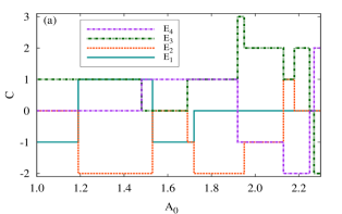
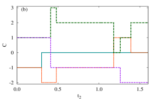
Figure 5: (Color online) (a) Topological phase diagram of the system shows rapid variation of phases with $A_{0}$, where $t_{2}$ and $\Omega$ are fixed at 1.0 and 10.0, respectively. Chern numbers of the four bands are plotted as a function of $A_{0}$. (b) Topological phase diagram of the system with respect to $t_{2}$. $A_{0}$ and $\Omega$ are fixed at 2.1 and 10.0, respectively. Summation of the Chern numbers over all the bands are zero, which is evident from the figures.

IV.2 Topological edge states

In order to examine whether the system obeys the ‘bulk-boundary correspondence’ rule, the effective Hamiltonian of a finite strip of the system is considered. Values of the parameter are taken as $t_{2}=1.0,A_{0}=2.1,\Omega=10$. The system remains in a particular CI phase for these values. To create edges in the system, periodic boundary condition along $\boldsymbol{a}_{2}$ direction is withdrawn, so that $k_{2}$ is no longer a good quantum number. Now, considering $N=50$ unit cells i.e. 200 sites along $a_{2}$ direction, the resulting $4N\times 4N$ Hamiltonian is diagonalized. The quasi-energy eigenvalues of the effective Hamiltonian are plotted as a function of $k_{1}$ in Fig 6. Density of states are also drawn in the side-panel to show that the spectrum has a true gap.

Evidently, additional states are found to appear within the band gaps, those actually connect the distinct bulk bands. These are known as the edge states, which are indeed localized in either left (blue curves) or right (red curves) edge of the finite lattice, as shown in the lower panel of Fig 6. It may be noted that the edge states are chiral in nature since the right-going states or the states with positive group velocity are localized in the right edge, and similarly, the left-going states with negative group velocity are always localized in the left edge.

Hence, the results are in accordance with the ‘bulk boundary correspondence’ rule which states that: sum of the Chern numbers up to the $i$-th band, $\nu_{i}=\sum_{j\leq i}C_{j}$ is equal to the number of pair of edge states in the gap Mook . It can be verified from the fact that the Chern numbers of the corresponding bands are ${-1,2,-1}$ in the ascending order of energy as shown in Fig 6. So, there must be one pair of edge states in each band gap.

\psfrag{x}{\text{\scriptsize{Right edge}}}\psfrag{y}{\text{\scriptsize{Left edge}}}\psfrag{q2}{\text{\scriptsize{$k_{1}$}}}\psfrag{wave-square}{\text{ \scriptsize{$|\psi(k_{1}\!\!=\!\!0)|^{2}$}}}\psfrag{Energy}{\text{\scriptsize{Energy($k_{1}$)}}}\psfrag{site}{\text{\scriptsize{Site}}}\psfrag{DOS}{\text{\tiny{DOS}}}\includegraphics[width=227.62204pt,height=199.16928pt]{Fig6.eps}

Figure 6: (Color online) Edge states of square-octagon lattice in the presence of circularly polarized light for the parameters $t_{2}=1.0,\Omega=10,A_{0}=2.1$ for $N=50$ unit cell along $k_{2}$. Chern numbers of the upper three bands are $C={-1,2,-1}$. The lowest band with $C=0$ is not shown in figure since the lowest band-gap does not accommodate any edge states. The side-panel indicates the density of states. Lower panel shows the probability density of left (blue) and right (red) going edge states with respect to site number of the strip for $k_{1}=0$. The colour of the edge state energies corresponds to the colour of particular edge where the probability density is concentrated.

V Summary and Discussion

The effect of circularly polarized light on the topology and band-structure of square-octagon lattice is studied by using the Floquet-Bloch theory. The system is topologically trivial in the absence of light with a pair of flat bands and quadratic band-touching points in its band-diagram. As soon as the system is exposed to circularly polarized light, flat bands become dispersive and the system is driven into non-trivial topological phase at the same time. Photo induced band structure exhibits true and pseudo gaps depending on the amplitude of light which eventually leads to the emergence of multiple topological phases with a variety of Chern number distribution. Thus a series of topological phase transitions is observed with the modulation of amplitude of the incident light and hopping strengths. The overall state of the system is identified either CSM or CI phase depending on the value of lattice filling. Those phases are topologically robust in a sense that no further change is observed with the variation of frequency as long as it is fixed in off-resonant regime. The frequency is always kept higher than the band-width of the undriven system to make sure that Floquet-Magnus expansion is always valid. Topological properties are characterized in terms of Chern numbers of distinct energy bands which is further justified with the behaviour of Hall conductance and evidence of edge states. Linearly polarized light has no effect on the topological properties of the system as it fails to break the TRS.

Previous investigation reveals that Dirac cones appear at the $\Gamma$ and M points in the absence of NNN hopping Ueda . The present study indicates that the system exhibits photo-induced CI phase in this case, for any values of lattice filling. So, it would be interesting to find the photo-induced topological properties of a particular model with different values of hopping strengths for intra- and inter-square-plaquette NN bonds on the square-octagon lattice. In this context, computation of finite-frequency optical conductivity will become useful for the experimental detection of topological phases. Additionally, further expansion of this work can be made by invoking further neighbour hoppings in this tight-binding model.

FTI phase has been observed on graphene with the help of opto-helical wave-guides Rechtsman and Floquet-Bloch bands have been found on the surface of the compound, Bi₂Se₃ Wang2 . In another development, optical lattices with ultracold atoms for two-dimensional honeycomb Panahi , checkerboard Wirth and kagomé Jo structures have been realized. So, the square-octagon optical lattice will hopefully become realizable in near future which, on the other hand, will pave the way for observation of these topological phases. However, square-octagon lattice based on real material had been come to light long ago in the context of antiferromagnetic compound, CaV₄O₉ Taniguchi . The spin-1/2 V⁴⁺ ions in this spin-liquid constitute square-octagon lattice structure. Meanwhile, quasi square-octagon structure has been found in $(10\bar{1}0)$ surface of functional material ZnO He . So, the recent trends of investigation indicate the realization of these findings very soon.

VI ACKNOWLEDGMENTS

AS acknowledges the CSIR fellowship, no. 09/096(0934) (2018), India. AKG acknowledges BRNS-sanctioned research project, no. 37(3)/14/16/2015, India.

Appendix A Derivation of $H_{\rm eff}$

To obtain the Fourier components of $H({\textbf{k}},t)$ (Eq 4), the coefficient of a particular term $-t_{1}\sum_{\textbf{k}}A_{\textbf{k}}^{\dagger}B_{\textbf{k}}$ in the expression of $H_{n}({\textbf{k}})$ becomes

$$\frac{1}{T}\int_{0}^{T}dte^{-in\Omega t}e^{-\frac{iA_{0}}{\sqrt{2}}(\sin(\Omega t)+\cos(\Omega t)}$$

$$=\frac{1}{T}\int_{0}^{T}dte^{-in\Omega t}e^{-iA_{0}\sin(\Omega t+\pi/4)},$$

$$=\frac{1}{2\pi}\int_{0}^{2\pi}d\tau e^{-in\tau}e^{in\pi/4}e^{-iA_{0}\sin(\tau)},$$

$$=J_{n}(-A_{0})e^{in\pi/4},$$ (13)

where $\tau=\Omega t+\pi/4$ and $\Omega T=2\pi$. Similarly, the coefficient of $-t_{1}\sum_{\textbf{k}}B_{\textbf{k}}^{\dagger}A_{\textbf{k}}$ becomes $J_{n}(A_{0})e^{in\pi/4}$. In the same way, all the other coefficients can be derived. The matrix elements of $4\times 4$ matrix $H_{n}(\textbf{k})$ are explicitly given by

$$H_{n}^{12}(\textbf{k}) =t_{1}J_{n}(-A_{0})e^{in\pi/4},$$ (14)

$$H_{n}^{21}(\textbf{k}) =t_{1}J_{n}(A_{0})e^{in\pi/4},$$

$$H_{n}^{13}(\textbf{k}) =t_{2}J_{n}(-\sqrt{2}A_{0})e^{in\pi/2}+J_{n}(A_{0})t_{1}e^{i(n\pi/2+k_{2}},$$

$$H_{n}^{31}(\textbf{k}) =t_{2}J_{n}(\sqrt{2}A_{0})e^{in\pi/2}+J_{n}(-A_{0})t_{1}e^{i(n\pi/2-k_{2}},$$

$$H_{n}^{14}(\textbf{k}) =t_{1}J_{n}(A_{0})e^{-in\pi/4},$$

$$H_{n}^{41}(\textbf{k}) =t_{1}J_{n}(-A_{0})e^{-in\pi/4},$$

$$H_{n}^{23}(\textbf{k}) =t_{1}J_{n}(A_{0})e^{-in\pi/4},$$

$$H_{n}^{32}(\textbf{k}) =t_{1}J_{n}(-A_{0})e^{-in\pi/4},$$

$$H_{n}^{24}(\textbf{k}) =t_{2}J_{n}(\sqrt{2}A_{0})+t_{1}J_{n}(-A_{0})e^{-ik_{1}},$$

$$H_{n}^{42}(\textbf{k}) =t_{2}J_{n}(-\sqrt{2}A_{0})+t_{1}J_{n}(A_{0})e^{ik_{1}},$$

$$H_{n}^{34}(\textbf{k}) =t_{1}J_{n}(A_{0})e^{in\pi/4},$$

$$H_{n}^{43}(\textbf{k}) =t_{1}J_{n}(-A_{0})e^{in\pi/4},$$

Now, applying the relations $J_{-n}(A_{0})={(-1)}^{n}J_{n}(A_{0})$ and $J_{n}(-A_{0})={(-1)}^{n}J_{n}(A_{0})$, matrix elements for the Fourier components of $H_{0}(\textbf{k})$, $H_{1}(\textbf{k})$ and $H_{-1}(\textbf{k})$ have been obtained and finally, $H_{\rm eff}$ is obtained by Eq 9.

References

- (1) M. Z. Hasan and C. L. Kane, Rev. Mod. Phys. 82, 3045 (2010).
- (2) S. Ryu, A. P. Schnyder, A. Furusaki and A. W. W. Ludwig, New Journal of Physics 12 (2010) 065010
- (3) D. J. Thouless, M. Kohomoto, P. Nightingale and M.den Nijs, Phys. Rev. Lett. 49, 405 (1982).
- (4) F. D. M. Haldane, Phys. Rev. Lett. 61, 2015 (1988).
- (5) C. L. Kane and E. J. Mele, Phys. Rev. Lett. 95, 146802 (2005).
- (6) T. Oka, and H. Aoki, Phys. Rev. B 79, 081406 (2009).
- (7) J. Inoue, Phys. Rev. B 81, 125412 (2010).
- (8) T. Kitagawa, E. Berg, M. Rudner, and E. Demler, Phys. Rev. B 82, 235114 (2010).
- (9) J. Inoue, and A. Tanaka, Phys. Rev. Lett. 105, 017401 (2010).
- (10) Y. Hatsugai, Phys. Rev. Lett. 71, 3697 (1993).
- (11) Y. Hatsugai, Phys. Rev. B 48, 11851 (1993).
- (12) A. Mook, J. Henk and I. Mertig, Phys. Rev. B 90, 024412 (2014).
- (13) S. K. Kim, H. Ochoa, R. Zarzuela and Y. Tserkovnyak, Phys. Rev. Lett. 117, 227201 (2016).
- (14) S. A. Owerre, J. Phys.: Condens. Matter 28, 386001 (2016).
- (15) H. Dehghani, T. Oka, and A. Mitra, Phys. Rev. B 91, 155422 (2015).
- (16) A. Kundu, H.A. Fertig, and B. Seradjeh, Phys. Rev. Lett. 113, 236803 (2014).
- (17) L. D’Alessio1, and M. Rigol, Nature Communications volume 6(1) 9336.
- (18) P. M. Perez-Piskunow, G. Usaj, C. A. Balseiro, and L. E. F. F. Torres, Phys. Rev. B 89, 121401(R) (2014).
- (19) S. Li, C.C. Liu and Y. Yao, New J. Phys. 20 (2018) 033025.
- (20) K.Saha, Phys. Rev. B 94, 081103(R) (2016).
- (21) N. Lindner, G. Refael, and V. Gaslitski, Nat. Phys. 7, 490 (2011).
- (22) M. Ezawa, Phys. Rev. Lett. 110, 026603 (2013).
- (23) A. Gomez-Leon and G. Platero, Phys. Rev. Lett. 110, 200403 (2013).
- (24) J. Cayssol, B. Dora, F. Simon, and R. Moessner, Physica Status Solidi (RRL) 7, 101 (2013).
- (25) L. Du, X. Zhou, and G. A. Fiete, Phys. Rev. B 95, 035136 (2017).
- (26) Y. Long and J. Ren, arXiv: 1706.01107.
- (27) M. S. Rudner, N. H. Lindner, E. Berg, and M. Levin, Phys. Rev. X 3, 031005 (2013).
- (28) S. A. Owerre, J. Phys. Commun. 1, 021002 (2017).
- (29) M. Kargarian and G. A. Fiete, Phys. Rev. B 82, 085106 (2010).
- (30) B. Pal, Phys. Rev. B. 98, 245116 (2018).
- (31) X. P. Liu, W. C. Chen, Y. F. Wang and C. D. Gong, J. Phys.: Condens. Matter 25 (2013) 305602.
- (32) Y. Yang et. al., Physics Letters A 382 (2018) 723–728.
- (33) Y. Yamashita, M. Tomura, Y. Yanagi and K. Ueda, Phys. Rev. B 88, 195104 (2013).
- (34) U. Yu, Phys. Rev. E 91, 062121 (2015).
- (35) G. Floquet, Ann. Sci. Ec. Normale Super. 12, 47 (1883).
- (36) M. Bukova, L. D’Alessio, and A. Polkovnikov, Adv. Phys. 64, 139 (2015).
- (37) T. Kitagawa, T. Oka, A. Brataas, L. Fu, and E. Demler, Phys. Rev. B 84, 235108 (2011).
- (38) G. Palumbo and K. Meichanetzidis, Phys. Rev. B. 92, 235106 (2015).
- (39) S. A. Owerre, arXiv: 1801.04932.
- (40) T. Fukui, Y. Hatsugai and H. Suzuki, Journal of the Physical Society of Japan 74, 1674 (2005).
- (41) M. C. Rechtsman, J. M. Zeuner, Y. Plotnik, Y. Lumer, D. Podolsky, F. Dreisow, S. Nolte, M. Segev, and A. Szameit, Nature 496, 196 (2013).
- (42) Y. H. Wang, H. Steinberg, P. J. Herrero and N. Gedik, Science 342, 453 (2013).
- (43) P. Soltan-Panahi et. al., Nat. Phys. 7 (2011) 434.
- (44) G. Wirth, M. Olschlager and A. Hemmerich, Nature Phys. 7, 147 (2010).
- (45) G. B. Jo et. al., Phys. Rev. Lett. 108, 045305 (2012).
- (46) S. Taniguchi et. al., J. Phys. Soc. Jpn. 64, 2758 (1995).
- (47) M. R. He, R. Yu, J. Zhu, Angew. Chem. 124 (2012) 78.