Data Masking with Privacy Guarantees

Abstract

We study the problem of data release with privacy, where data is made available with privacy guarantees while keeping the usability of the data as high as possible — this is important in health-care and other domains with sensitive data. In particular, we propose a method of masking the private data with privacy guarantee while ensuring that a classifier trained on the masked data is similar to the classifier trained on the original data, to maintain usability. We analyze the theoretical risks of the proposed method and the traditional input perturbation method. Results show that the proposed method achieves lower risk compared to the input perturbation, especially when the number of training samples gets large. We illustrate the effectiveness of the proposed method of data masking for privacy-sensitive learning on $12$ benchmark datasets.

Introduction

In domains like healthcare or finance, data can be sensitive and private. There are several scenarios where a dataset needs to be shared while protecting sensitive parts of the data. For example, consider a medical study where a group of patients with a particular medical condition are being studied. The identifying data of some patients (e.g., those with a rare disease) may need to be masked while sharing their records with a wider group of medical researchers. However, when the patient records are processed by clinical decision support tools, we want the machine learning (ML) models in the tools to have similar performance on the masked data as they would on the original data.

Several approaches have been proposed to preserve privacy of data, e.g., by anonymization (?), by generalization (?). Methods for differential-privacy include adding Laplace-noise (?), modifying the objective (?), and posterior sampling (?; ?). Privacy-preserving data publishing transforms sensitive data to protect it against privacy attacks while supporting effective data mining tasks (?). Differentially private data release (?) presents an anonymization algorithm that satisfies the $\epsilon-$differential privacy model, while other methods of data release (?; ?) group the data and add noise to the partition counts. However, these techniques don’t explicitly try to maintain the accuracy of a model. Our approach masks training samples with less sensitive ones with privacy guarantee, while ensuring that the classifier trained on the masked data reaches accuracy similar to the classifier trained on the original data. Moreover, compared to publishing masked classifier, publishing masked data enables other types of classifiers to be trained by the user. There are also query-based data masking methods for a classifier, which are sparse vector techniques for generating masked data using a query that the gradient of the masked data is zero (?; ?; ?; ?). However, when the gradient computation is complicated, designing a method to achieve a zero gradient can be tricky.

We have three main contributions in this paper. First, we propose a novel algorithm of data masking for privacy-sensitive learning. Second, we provide a theoretical guarantee explaining why the proposed method is more suitable for a large number of training samples than a traditional input perturbation method. Finally, we illustrate the efficacy of our method considering logistic regression as an example classifier, on both synthetic and $12$ benchmark datasets.

Problem setting

Goal: Assume we train a model parameterized by ${\bf w}\in\mathbb{R}^{d}$ on a dataset $\mathbb{D}_{train}=\{{\bf x}_{i},y_{i}\}_{i=1}^{N}$, where ${\bf x}_{i}\in\mathbb{X}=\mathbb{R}^{d}$, $y_{i}\in\mathbb{Y}=\{-1,1\}$, and $d$ is the number of features. The goal of our data publishing algorithm $\mathbb{A}$ is generating a masked training dataset $\mathbb{D}_{masked}=\{{\bf x}^{\prime}_{i},y_{i}\}_{i=1}^{N}$, where ${\bf x}^{\prime}_{i}\in\mathbb{X}$, such that: (a) $\mathbb{D}_{masked}$ is as different as possible from $\mathbb{D}_{train}$, but (b) the model trained on $\mathbb{D}_{masked}$ gives us parameters ${\bf w}^{\prime}$ that are close to the original parameters ${\bf w}$ of the model trained on $\mathbb{D}_{train}$.

This paper outlines an approach for achieving this goal. Before that, we review several concepts of data publishing with privacy and the core formulation of logistic regression.

Data publishing with differential privacy (DPDP)

We first begin with the concept of data publishing with differential privacy (DPDP). We consider two datasets of $N$ training samples, $\mathbb{D}_{train1}=\{{\bf x}_{1i},y_{1i}\}_{i=1}^{N}$ and $\mathbb{D}_{train2}=\{{\bf x}_{2i},y_{2i}\}_{i=1}^{N}$, which are different at only one sample: without loss of generality, assume ${\bf x}_{1i}={\bf x}_{2i}$ and $y_{1i}=y_{2i}$ for $i=\{1,2,\dots,N-1\}$, and ${\bf x}_{1N}\neq{\bf x}_{2N}$ and (or) $y_{1N}\neq y_{2N}$. A data publishing algorithm $\mathbb{A}$ is said to be $\epsilon$-private (?) if

$$\frac{p\big{(}\mathbb{A}(\mathbb{D}_{train1})=\mathbb{O}\big{)}}{p(\mathbb{A}\big{(}\mathbb{D}_{train2})=\mathbb{O}\big{)}}<e^{\epsilon},$$

where $\mathbb{O}=\{{\bf x}^{\prime}_{i},y_{i}\}_{i=1}^{N}$ is a particular output of the data publishing algorithm $\mathbb{A}$. Intuitively, differential privacy guarantees that for small $\epsilon$, the output of $\mathbb{A}$ is not sensitive to the existence of a single sample in the dataset. In this setting, the attacker has less chance to infer details about a particular training sample in the data. In this work we focus on differential privacy for masked data generation where the machine learning algorithm we consider is logistic regression (?).

Core formulation of logistic regression

Logistic Regression: We are given a training dataset $\mathbb{D}_{train}$. The goal for training a logistic regression classifier is finding a mapping function between a sample in $\mathbb{R}^{d}$ and a label in $\{1,-1\}$. Specifically, we model the relation among a sample ${\bf x}_{i}$ and its label $y_{i}$ as

$$p(y_{i}|{\bf x}_{i},{\bf w})=\frac{e^{y_{i}{\bf w}^{T}{\bf x}_{i}}}{1+e^{y_{i}{\bf w}^{T}{\bf x}_{i}}}.$$

Assuming samples are i.i.d., the log-likelihood for the training samples is

$$\mathbb{L}_{\lambda}({\bf w})=\frac{1}{N}\sum_{i=1}^{N}\Big{[}\big{(}y_{i}{\bf w}^{T}{\bf x}_{i}\big{)}-\log(1+e^{y_{i}{\bf w}^{T}{\bf x}_{i}})\Big{]}+\lambda\frac{||{\bf w}||^{2}}{2},$$ (1)

with $\lambda$ is the regularization parameter and $||\cdot||$ denotes the 2-norm.

Training logistic regression: In logistic regression, training is done by finding the parameter ${\bf w}$ that maximizes the log-likelihood in (1), i.e., the gradient of $\mathbb{L}_{\lambda}$ at ${\bf w}$ is $0$, as follows:

$$\frac{\partial\mathbb{L}_{\lambda}({\bf w})}{\partial{\bf w}}=\frac{1}{N}\Big{[}\sum_{i=1}^{N}\Big{[}y_{i}-p(y_{i}=1|{\bf x}_{i},{\bf w})\Big{]}{\bf x}_{i}\Big{]}+\lambda{\bf w}=0.$$ (2)

For various logistic regression optimization techniques to make the above gradient $0$, please refer to (?).

DPDP by Masked Data Generation

In this section, we describe how to generate masked samples for logistic regression.

Adding Laplace noise to the classifier

Unlike previous approaches of adding noise to the data then publishing noisy data, we consider a novel approach: we first train a classifier on the original data, and then add Laplace noise to the classifier. The motivation for adding noise is that in differential privacy, the goal is to make similar output for any two neighbor datasets $\mathbb{D}_{1}$ and $\mathbb{D}_{2}$ so that attacker cannot infer about the existence of any single training sample. Since the classifiers trained on two datasets $\mathbb{D}_{1}$ and $\mathbb{D}_{2}$ are not equal, adding Laplace noise to the parameters of those classifiers would account for that difference, and with some probability those classifiers after adding noise would be equal. Subsequently, we generate and publish a masked dataset such that the gradient of the log-likelihood for the noisy classifier is $0$. The work flow of the proposed framework is illustrated in Fig. 1(a). In comparison, the work flow of traditional data publishing methods by perturbation is shown in Fig. 1(b).

Figure 1: The work flow of the proposed method and traditional data publishing methods.

Generating masked data

We generate masked data $\mathbb{O}=\{{\bf x}^{\prime}_{i}\}_{i=1}^{N}$ such that the gradient of the log-likelihood of $\mathbb{O}$ for the aforementioned noisy classifier ${\bf w}^{\prime}$ is $0$. The optimal condition for masked data is the following:

$$\frac{1}{N}\Big{[}\sum_{i=1}^{N}\Big{[}y_{i}-p(y_{i}=1|{\bf x}^{\prime}_{i},{\bf w}^{\prime})\Big{]}{\bf x}^{\prime}_{i}\Big{]}+\lambda{\bf w}^{\prime}=0,$$ (3)

where the masked samples $\{{\bf x}^{\prime}_{i},y^{\prime}_{i}\}$(s) are unknown. To evaluate the optimality of the set $\mathbb{S}$ of masked samples w.r.t. ${\bf w}^{\prime}$, we use the 2-norm of the gradient:

$$\mathcal{N}(\mathbb{S})=\Big{|}\Big{|}\sum_{i=1}^{N}\Big{(}y_{i}-p(y_{i}=1|{\bf x}^{\prime}_{i},{\bf w}^{\prime}){\bf x}^{\prime}_{i}\Big{)}+N\lambda{\bf w}^{\prime}\Big{|}\Big{|}^{2}$$

We start with an initial set of training samples $\mathbb{S}$ then iteratively add new sample to $\mathbb{S}$. The criteria to evaluate the new sample is the 2-norm of the gradient of $\mathbb{S}$ after including the new sample.

Algorithm 1 outlines our proposed Masked Data Generation algorithm. The algorithm terminates when the number of samples in $\mathbb{S}$ reaches $N$.

Algorithm 1 Masked Data Generation

$N$ training samples $\mathbb{D}_{train}=\{{\bf x}_{i}\}_{i=1}^{N}$, $\epsilon$

$N$ masked training samples $\mathbb{O}=\{{\bf x}^{\prime}_{i}\}_{i=1}^{N}$.

 Step 1: Train Logistic regression classifier ${\bf w}$, as in (2).

Step 2: Add Laplace noise to the classifier ${\bf w}^{\prime}={\bf w}+\eta$, where $||\eta||$c$\sim e^{-\frac{\lambda N\epsilon}{2}||\eta||}$, where $c$ is a normalized constant.

Step 3: $\mathbb{S}=\{\emptyset\}$. Incrementally generate masked samples.

while $cardinality(\mathbb{S})\leq N$ do

Find an outliers $\{{\bf x}^{\prime}_{m}\}$ reducing the 2-norm of the gradient of $\mathbb{S}$ the most, using Gradient Descent (5)

Add the new sample $\mathbb{S}=\mathbb{S}\bigcup\{{\bf x}^{\prime}_{m}\}$

end while

Return $\mathbb{O}=\mathbb{S}$;

Iteratively generating masked samples

In this section, we present the gradient descent method to iteratively generate masked samples. In particular, given the current set of masked samples $\mathbb{S}$, we need to find the next masked sample $\{{\bf x}^{\prime}_{m}\}$ such that the 2-norm of the gradient of the set $\mathbb{S}\bigcup\{{\bf x}^{\prime}_{m}\}$ is close to $0$ as possible.

For simplicity of notation, denote $\sum_{{\bf x}^{\prime}_{i}\in\mathbb{S}}\Big{(}y_{i}-p(y_{i}=1|{\bf x}^{\prime}_{i},{\bf w}){\bf x}^{\prime}_{i}\Big{)}+N\lambda{\bf w}=g$ as the current gradient of the current masked samples. Consequently, we need to find the next masked sample $\{{\bf x}^{\prime}_{m}\}$ minimizing the following objective

$$\mathcal{N}({\bf x}^{\prime}_{m})=||\big{(}y_{m} - \frac{e^{y_{m}{\bf w}^{T}{\bf x}^{\prime}_{m}}}{1+e^{{\bf w}^{T}{\bf x}^{\prime}_{m}}}\big{)}{\bf x}^{\prime}_{m}+g||^{2}.$$ (4)

To minimize (4), we use backtracking gradient descent. The gradient is computed as

$$\frac{\partial\mathcal{N}({\bf x}^{\prime}_{m})}{\partial{\bf x}^{\prime}_{m}}=2\Big{(}\big{(}y_{m}-\frac{e^{y_{m}{\bf w}^{T}{\bf x}^{\prime}_{m}}}{1+e^{{\bf w}^{T}{\bf x}^{\prime}_{m}}}\big{)}{\bf x}^{\prime}_{m}+g\Big{)}\times$$

$$\Big{(}(y_{m}-\frac{e^{{\bf w}^{T}{\bf x}^{\prime}_{m}}}{1+e^{{\bf w}^{T}{\bf x}^{\prime}_{m}}})\mathbb{I}-{\bf w}^{T}{\bf x}^{\prime}_{m}\frac{e^{{\bf w}^{T}{\bf x}^{\prime}_{m}}}{(1+e^{{\bf w}^{T}{\bf x}^{\prime}_{m}})^{2}}\Big{)},$$ (5)

where $\mathbb{I}$ is the identity matrix in $\mathbb{R}^{d\times d}$. Note that, we can generalize our algorithm to $C$ classes, with $C>2$, as follows

$$\frac{\partial\mathcal{N}}{\partial{\bf x}^{\prime}_{m}}=\sum_{c=1}^{\mathcal{C}}2\Big{(}[I(y_{m}=c)-p(y_{m}=c|{\bf x}^{\prime}_{m},{\bf w})]{\bf x}^{\prime}_{m}+g_{c}\Big{)}\times$$

$$\Big{(}[I(y_{m}=c)-p(y_{m}=c|{\bf x}^{\prime}_{m},{\bf w})]-$$

$$\sum_{l=1}^{C}[p(y_{m}=c|{\bf x}^{\prime}_{m},{\bf w})p(y_{m}=l|{\bf x}^{\prime}_{m},{\bf w})({\bf w}_{c}-{\bf w}_{l})^{T}{\bf x}^{\prime}_{m})]\Big{)}.$$

Computational complexity: The computational complexity of the proposed algorithm is linear in term of number of added samples.

Intuition: Most differential privacy algorithms for data publishing modify the data by adding uniform noise, e.g., as in Fig. 1(b), which may change the original data manifold closer to a uniform manifold and may not be optimized for any particular machine learning model.

Comparison to classifier publishing: The proposed approach has an advantage over other traditional approaches. In particular, assuming a non-empty initialized set of training samples $\mathbb{S}$ in Step $3$ of Algorithm 1, the proposed method adds fake samples with completely different manifold to the dataset. For example, assume we want to preserve the privacy of a dataset consisting of non-diabetes patients and sensitive type-1 diabetes patients. We can initially add non-sensitive type-2 diabetes data samples, thereby preserving the privacy of the type-1 diabetes patients. Moreover, by iteratively adding masked samples, a classifier that is trained on the original data will be quite close to the classifier trained on the new masked data. Compared to publishing the noisy classifier as in (?), the proposed data masking method allows users to benefit from real data, i.e., in this case non-diabetes and type-2 diabetes data, and train other types of classifiers on them.

Privacy guarantee of Masked Data Generation

There are two aspects of a data publishing algorithm. First, we need to guarantee that the algorithm is $\epsilon$-private. In particular, is the algorithm sensitive to the existence of a single sample in two datasets that are different only at that sample? Second, we would like to assess how the utility of the published dataset changes with changing $\epsilon$. The following Proposition answers the first question.

Proposition 1

If $||{\bf x}_{i}||\leq 1,\forall i$, then Algorithm 1 is $\epsilon$-private.

Utility of Masked Data Generation with changing $\epsilon$

We next consider the utility aspect of the masked dataset $\mathbb{O}$ with different values of $\epsilon$. We consider the utility of the published data to be how well the classifier trained on the published data is close to the classifier trained on the original data.

Let us suppose that training logistic regression on the original dataset $\mathbb{D}_{train}$ and the masked dataset $\mathbb{O}$ gives us parameters ${\bf w}$ and ${\bf w}^{\prime}$, respectively. We are interested in comparing the $0/1$ risk (?) of the classifier trained on masked data (${\bf w}^{\prime}$), to the $0/1$ risk of the classifier trained on original data (${\bf w}$). Note that logistic regression is classification calibrated (?), which means that minimizing the negative log-likelihood leads to minimizing the $0/1$ risk. Thus, it is sufficient to compare the log-likelihood $\mathbb{L}_{\lambda}$ of ${\bf w}^{\prime}$ compared to that of ${\bf w}$.

Proposition 2

With probability $1-\delta$, $\mathbb{L}_{\lambda}({\bf w}^{\prime})-\mathbb{L}_{\lambda}({\bf w})\leq\frac{1}{2}(\frac{2d\log(\frac{d}{\delta})}{\lambda N\epsilon})^{2}(\lambda+1)$.

From Lemma 2, the classifier trained on masked data improves when $N$ is larger.

DPDP by Input Perturbation

In this section, we consider a classical and natural algorithm to publish data (?; ?). The algorithm is quite simple: it directly adds noise $\eta\sim e^{\frac{-\epsilon||\eta||}{2}}$ to each input sample. The detailed algorithm is shown in Algorithm 2. Similar to Algorithm 1, in the rest of this section we consider the privacy and the utility of the input perturbation algorithm when $\epsilon$ changes.

Privacy guarantee of Input Perturbation

We first show that Algorithm 2 is $\epsilon$-private.

Proposition 3

If $||{\bf x}_{i}||\leq 1,\forall i$, then algorithm 2 is $\epsilon$-private.

Algorithm 2 Input Perturbation

$N$ training samples $\mathbb{D}_{train}=\{{\bf x}_{k}\}_{k=1}^{N}$, $\epsilon$

$N$ masked training samples $\mathbb{O}=\{{\bf x}^{\prime}_{k}\}_{k=1}^{N}$

 

while $k<N$ do

$\eta\sim e^{\frac{-\epsilon||\eta||}{2}}$

${\bf x}_{k}^{\prime}={\bf x}_{k}+\eta$

$k=k+1$

end while

Return $\mathbb{O}=\{{\bf x}_{k}^{\prime}\}_{k=1}^{N}$

Utility of Input Perturbation with changing $\epsilon$

Similar to Section Utility of Masked Data Generation with changing $\epsilon$, we consider the log-likelihood of the classifier ${\bf w}^{\prime}$ trained on perturbed data. We are going to bound the log-likelihood w.r.t. the original data $\mathbb{L}_{\lambda}({\bf w}^{\prime})-\mathbb{L}_{\lambda}({\bf w})$. We begin with the following Proposition.

Lemma 4

(?). Let $G({\bf w})$ be a convex function and $g({\bf w})$ be a function with $||\nabla g({\bf w})||\leq g_{1}$ and $\min_{v}\min_{{\bf w}}||v^{T}\nabla^{2}(G+g)({\bf w})v||\geq G_{2}$. Let ${\bf w}=\arg\min G({\bf w})$ and ${\bf w}^{\prime}=\arg\min G({\bf w})+g({\bf w})$. Then $||{\bf w}^{\prime}-{\bf w}||\leq\frac{g_{1}}{G_{2}}$.

Proposition 5

With probability $1-\delta$, $\mathbb{L}_{\lambda}({\bf w}^{\prime})-\mathbb{L}_{\lambda}({\bf w})\leq\frac{1}{2}(\frac{2d\log\frac{d}{\delta}}{\lambda\epsilon})^{2}(\lambda+1)$.

From Proposition 5, the classifier trained on perturbed data does not improve when $N$ is larger, as we see in Proposition 2.

Experiments

We compare the performance of our Masked Data Generation method in Algorithm 1 to the Input Perturbation method in Algorithm 2, on both synthetic and real datasets.

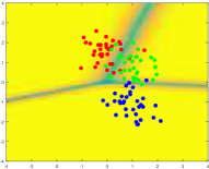
(a) True training samples

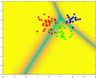
(b) Initially masked samples set $\mathbb{S}$

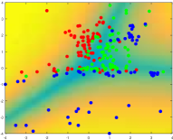
(c) Final masked samples

Figure 2: (a) Original training samples, (b) Initially masked training samples, (c) Final masked samples using Algorithm 1

(a) True training samples

(b) Initially masked samples set $\mathbb{S}$

(c) Final masked samples using Algorithm 1

(d) True training ${\bf w}$

(e) Initially masked ${\bf w}$ set $\mathbb{S}$

(f) Masked ${\bf w}$

Figure 3: (a) True training samples, (b) Initially masked samples in $\mathbb{S}$, (c) Final masked samples using Algorithm 1, and their corresponding ${\bf w}$’s visualization (d-f) on MNIST datasets. We have digits from $0,1,3$ and we would like to replace $3$ with $6$ using some fake samples.

(a) True training samples

(b) Initially masked samples set $\mathbb{S}$

(c) Final masked samples using Algorithm 1

(d) True training ${\bf w}$

(e) Initially masked ${\bf w}$

(f) Masked ${\bf w}$

Figure 4: (a) True training samples, (b) Initially masked samples in $\mathbb{S}$, and (c) Final masked samples using Algorithm 1, and their corresponding ${\bf w}$’s visualization (d-f) on MNIST datasets. We have digits from $0,1,4$ and we would like to replace $4$ with $8$ using some fake samples.

Results on toy data

Datasets: In this section, the effectiveness of the proposed method is illustrated on a 2D toy dataset. We sample $100$ training samples from three normal distributions. The $1$st class comes from $\mathcal{N}([0;1.5]^{T},0.25I)$, the $2$nd class comes from $\mathcal{N}([1;1]^{T},0.25I)$, and the $3$rd class comes from $\mathcal{N}([1;-1]^{T},0.25I)$, as shown in Fig. 2(a). Assume that samples from the $3$rd class is sensitive.

Setting: We initialize the samples in the masked dataset from a class with a different manifold for the $3$rd class. In particular, we first add to the published dataset a fake class $3$ with a totally different distribution manifold from the original class $3$, e.g., $\mathcal{N}([2;2]^{T},0.25I)$ instead of $\mathcal{N}([1;-1]^{T},0.25I)$, as shown in Fig. 2(b). We then run the masked data generation method with non-empty training samples set $\mathbb{S}$ as in Algorithm 1.

Results: The samples generated from the proposed method are shown in Fig. 2(c). From Fig. 2(c), to accommodate for the shift in distribution manifold of class 3 from $[2;2]$ to $[1;-1]$, many other fake samples of class $3$ are added in the bottom of Fig. 2(c).From Fig. 2(c), we observe the usefulness of regularization, since less masked samples are on the boundary. From Fig. 2(c) and Fig. 2(a), the generated samples from class $3$ is significantly different from the original true samples from class $3$, which implies that the data is private. However, the resulting classifier or the boundary learned from the three classes are almost similar for original data and published data. As a result, users are still able to access original real data from classes $1$ and $2$, and at the same time achieve the classifier for class $3$ which is private now.

Results on MNIST digits data

In this section, we consider the effectiveness of the proposed algorithm on the MNIST handwritten digit dataset.

Datasets: We use PCA to reduce the dimensionality of the data to 25. Similar to the toy example, we select samples from three digits, e.g., three digits $\{0,1,3\}$ as in Fig. 3(a), and three digits $\{0,1,4\}$ as in Fig. 4(a). The corresponding classifier learned from three digits $\{0,1,3\}$ is shown in Fig. 3(d), and from three digits $\{0,1,4\}$ is shown in Fig. 4(d). From those figures, e.g., in Fig. 3(d), the visualized classifier represents the three corresponding digits $\{0,1,3\}$.

Setting: We first explain how to generate a non-empty initially masked training samples $\mathbb{S}$ in Algorithm 1. In particular, the first two digits from the initially masked training samples are the same as the two digits of the original training samples. For example, we still uses samples from digits $0$ and $1$ for initially masked training samples as in Fig. 3(b). However, for the last digit of the initially masked training samples, we use a totally different digit from the last digit of the true training samples. For example, we use digit $6$ instead of digit $3$ as the last digit as in Fig. 3(b). The corresponding classifier learned from the initially masked training samples $\mathbb{S}$ is visualized in Fig. 4(e).

Result: We then iteratively add masked training samples into $\mathbb{S}$ using the masked data generation method in Algorithm 1. The masked samples generated by Algorithm 1 into $\mathbb{S}$ are shown in Fig. 3(c). Note that several samples among them remove the effect of digit $6$, e.g., the $4$th sample from the left in the first row of Fig. 3(c). On another hand, several among them add the effect of digit $3$ back to the classifier, e.g., the image at the bottom right of Fig. 3(c). Moreover, because of the adding masked samples, the classifier learned from the masked training samples is similar to the original classifier learned from the original training samples. For example, the classifier in Fig. 3(f) is similar to the classifier in Fig. 3(d).

A similar visualization example is shown in Fig. 4, where the original training samples are digit $\{0,1,4\}$ as in Fig. 4(a), the initially masked training samples in $\mathbb{S}$ are digit $\{0,1,8\}$ as in Fig. 4(b), and after generating masked samples, the classifier of the masked data as in Fig. 4(f) is similar to the classifier of original data as in Fig. 4(d).

(a) Adult income

(b) German credit

(c) Age of Abalone

(d) Wave form

(e) AUS credit

(f) Breast cancer

(g) Blood transfusion

(h) Heart disease

(k) Diabetics

(i) Mammographic

(j) SpliceDNA

(m) Image

Figure 5: The accuracy and privacy ($\epsilon$ in log-scale) trade off for $12$ benchmark datasets.

Results on UCI datasets

Datasets: We demonstrate the effectiveness of the proposed method on several UCI datasets in sensitive domains.

Evaluation Measure: For all datasets, we uniformly select a validation set $V=\{{\bf x}_{i}\}_{i=1}^{n_{val}}$ of samples from two classes. We denote the ground truth labels for these samples as $L_{true}$. Using ${\bf w}^{\prime}$, the classifier trained on masked data, we predict the labels for the validation set, namely $V_{masked}$. Then, we compute the accuracy of ${\bf w}^{\prime}$ as the fraction of cases where $V_{masked}$ matches $L_{true}$.

Setting: We consider the regularization parameter $\lambda=0.5$. Moreover, to evaluate the effectiveness of the proposed method and the input perturbation method when the number of training samples increases, we consider two cases: $N=100$ and $N=200$. We vary the value of $\epsilon$ in the set $\{0.1,0.2,0.5,1,2,\dots,20,50\}$, e.g., log-scale. For each value of $\epsilon$, we generate $50$ training datasets, run the proposed masked data generation Algorithm 1 and the input perturbation Algorithm 2 on each dataset, then report the mean and standard deviation accuracy of both algorithms. We also evaluate the accuracy using the classifier after adding Laplace noise, i.e., after Step 2 of Algorithm 1, which is named as output perturbation.

Analysis: As shown in Fig. 5, first, as $\epsilon$ increases, the accuracy of both methods increase. Additionally, for a particular value of $\epsilon$, the proposed method works better than input perturbation algorithm. Moreover, as $N$ increases from $100$ to $200$, the proposed method gets higher accuracy for the same value of $\epsilon$. In contrast, the accuracy of the input perturbation method does not change much as $N$ increases. Furthermore, note that the input perturbation method only updates the data independently from the machine learning model. In contrast, the data generated by the proposed method is directly tied to the model, e.g., logistic regression with a particular value of $\lambda$, which may lead to higher accuracy. Moreover, the performance of the classifier trained on masked samples is comparable to those of the classifier trained on original training samples then adding Laplace noise, i.e., after Step 2 of Algorithm 1. The results indicate that the proposed masked data generation Algorithm 1 is able to create masked samples with corresponding classifier close to the perturbed classifier.

Conclusions

In this paper, we proposed a data masking technique for privacy-sensitive learning. The main idea is to iteratively find masked data such that the gradient of the likelihood on the classifier with regarding to the masked data is zero. Our theoretical analysis showed that the proposed technique achieves higher utility compared to a traditional input perturbation technique. Experiments on multiple real-world datasets also demonstrated the effectiveness of the proposed method.

Appendices

Proof for Proposition 1. Assume there are two training datasets $\mathbb{D}_{1}=\{{\bf x}_{1i}\}_{i=1}^{N}$ and $\mathbb{D}_{2}=\{{\bf x}_{2i}\}_{i=1}^{N}$, which are different at only one sample. Without the loss of generality, we assume ${\bf x}_{1i}={\bf x}_{2i}$ for $i=\{1,2,\dots,N-1\}$, and ${\bf x}_{1N}\neq{\bf x}_{2N}$. Assume the outputs of Algorithm 1 is $\mathbb{O}=\{{\bf x}^{\prime}_{1},{\bf x}^{\prime}_{2},\dots,{\bf x}^{\prime}_{N}\}$. Consider the ratio $\frac{p(\mathbb{O}|\mathbb{D}_{1})}{p(\mathbb{O}|\mathbb{D}_{2})}$. We assume that in Step $3$ we can find the output $\mathbb{O}$ such that the gradient of logistic regression objective w.r.t. ${\bf w}^{\prime}$ is exactly $0$. For the classifier in Step $2$, we consider ${\bf w}^{\prime}=a_{1}$ for the first dataset $\mathbb{D}_{1}$ and ${\bf w}^{\prime}=a_{2}$ for the second dataset $\mathbb{D}_{2}$. Using the fact that the log-likelihood of logistic regression is convex, and $a_{1}$ and $a_{2}$ are both optimal classifiers of the published data $\mathbb{O}$, thus $a_{1}=a_{2}=a$. Then, the ratio $\frac{p(\mathbb{O}|\mathbb{D}_{1})}{p(\mathbb{O}|\mathbb{D}_{2})}$ is computed as:

$$\frac{p(\mathbb{O}|\mathbb{D}_{1})}{p(\mathbb{O}|\mathbb{D}_{2})}=\frac{p(\mathbb{O}|{\bf w}^{\prime}=a)p({\bf w}^{\prime}=a|\mathbb{D}_{1})}{p(\mathbb{O}|{\bf w}^{\prime}=a)p({\bf w}^{\prime}=a|\mathbb{D}_{2})}=\frac{p({\bf w}^{\prime}=a|\mathbb{D}_{1})}{p({\bf w}^{\prime}=a|\mathbb{D}_{2})}.$$

Assume ${\bf w}_{1}=b_{1}$ and ${\bf w}_{1}=b_{2}$ are the optimal classifiers for $\mathbb{D}_{1}$ and $\mathbb{D}_{2}$ after Step $1$. Therefore, because of Laplace noise in Step $2$, $b_{1}+\eta_{1}=b_{2}+\eta_{2}=a\Rightarrow\frac{p({\bf w}^{\prime}=a|\mathbb{D}_{1})}{p({\bf w}^{\prime}=a|\mathbb{D}_{2})}=\frac{p(\eta=\eta_{1})}{p(\eta=\eta_{2})}=e^{-\frac{\lambda N\epsilon}{2}(||\eta_{1}||-||\eta_{2}||)}$. Consequently, $\frac{p(\mathbb{O}|\mathbb{D}_{1})}{p(\mathbb{O}|\mathbb{D}_{2})}\leq e^{\frac{\lambda N\epsilon}{2}(||b_{1}||-||b_{2}||)}\leq e^{\frac{\lambda N\epsilon}{2}(||b_{1}-b_{2}||)}$. The sensitivity of logistic regression with $N$ samples and regularization parameter $\lambda$ is atmost $\frac{2}{\lambda N}$ (?) $\Rightarrow\frac{p(\mathbb{O}|\mathbb{D}_{1})}{p(\mathbb{O}|\mathbb{D}_{2})}\leq e^{\epsilon}$, which completes the proof. ∎

Proof for Proposition 2. Since ${\bf w}^{\prime}$ is achieved from ${\bf w}$ by adding Laplace noise, $||{\bf w}^{\prime}-{\bf w}||$ is bounded. So, $\mathbb{L}_{\lambda}({\bf w}^{\prime})-\mathbb{L}_{\lambda}({\bf w})$ is bounded using Taylor series. The rest of the proof follows from Lemma 1 in (?). ∎

Proof for Proposition 3. Assume there are two training datasets $\mathbb{D}_{1}=\{{\bf x}_{1i}\}_{i=1}^{N}$ and $\mathbb{D}_{2}=\{{\bf x}_{2i}\}_{i=1}^{N}$, which are different at only one sample, e.g., without the loss of generality, we assume ${\bf x}_{1i}={\bf x}_{2i}$ for $i=\{1,2,\dots,N-1\}$, and ${\bf x}_{1N}\neq{\bf x}_{2N}$. Assume the outputs of of Algorithm 2 is $\mathbb{O}=\{{\bf x}^{\prime}_{1},{\bf x}^{\prime}_{2},\dots,{\bf x}^{\prime}_{N-1},{\bf x}^{\prime}_{N}\}$. Consider the ratio

$$\frac{p(\mathbb{O}|\mathbb{D}_{1})}{p(\mathbb{O}|\mathbb{D}_{2})} = \frac{p({\bf x}^{\prime}_{1}|{\bf x}_{1})\dots p({\bf x}^{\prime}_{N-1}|{\bf x}_{N-1})p({\bf x}^{\prime}_{N}|{\bf x}_{1N})}{p({\bf x}^{\prime}_{1}|{\bf x}_{1})\dots p({\bf x}^{\prime}_{N-1}|{\bf x}_{N-1})p({\bf x}^{\prime}_{N}|{\bf x}_{2N})}$$

$$=\frac{e^{-0.5\epsilon||{\bf x}^{\prime}_{N}-{\bf x}_{1N}||}}{e^{-0.5\epsilon||{\bf x}^{\prime}_{N}-{\bf x}_{2N}||}}\leq e^{0.5\epsilon||{\bf x}_{1N}-{\bf x}_{2N}||}\leq e^{\epsilon},$$

where the last equation is from the fact that $||{\bf x}_{i}||\leq 1,\forall i$. Thus, the input perturbation algorithm is $\epsilon$-private. ∎

Proof for Proposition 5. The proof is similar to (?). For the sake of completeness, following Lemma 4, define $G({\bf w})=H_{2}({\bf w})+\lambda\frac{||w||^{2}}{2}$ and $g=H^{{}^{\prime}}_{2}({\bf w})-H_{2}({\bf w})$, where $H^{{}^{\prime}}_{2}({\bf w})=\frac{1}{N}\sum_{i=1}^{N}\Big{[}\big{(}y_{i}{\bf w}^{T}{\bf x}^{\prime}_{i}\big{)}-\log(\sum_{l=1}^{C}e^{{\bf w}^{T}{\bf x}^{\prime}_{i}})\Big{]}$ and $H_{2}({\bf w})=\frac{1}{N}\sum_{i=1}^{N}\Big{[}\big{(}y_{i}{\bf w}^{T}{\bf x}_{i}\big{)}-\log(\sum_{l=1}^{C}e^{{\bf w}^{T}{\bf x}_{i}})\Big{]}$. Then, $||\nabla g||=||\frac{1}{N}\Big{[}\sum_{i=1}^{N}\Big{(}-(y_{i}-p(y_{i}=1|{\bf x}_{i},{\bf w})\Big{)}{\bf x}^{\prime}_{i}+\sum_{i=1}^{N}\Big{(}-(y_{i}-p(y_{i}=1|{\bf x}_{i},{\bf w})\Big{)}{\bf x}_{i}\Big{]}||\leq\frac{1}{N}\sum_{i=1}^{N}||{\bf x}^{\prime}_{i}-{\bf x}_{i}||\leq(N2d\log\frac{d}{\delta})/(N\epsilon)=2d\log\frac{d}{\delta}/\epsilon$, where the last inequality comes from the fact $||{\bf x}^{\prime}_{i}-{\bf x}_{i}||\sim e^{\frac{-\epsilon||\eta||}{2}}$ and ${\bf x}^{\prime}_{i}$, ${\bf x}_{i}\in\mathbb{R}^{d}$. Note that even though $||{\bf x}_{i}||$ is upper bounded by $1$ $\forall i$, $||{\bf x}^{\prime}_{i}||$ is not upper bounded by $1$ since ${\bf x}^{\prime}_{i}={\bf x}_{i}+\eta$ where $\eta\sim e^{\frac{-\epsilon||\eta||}{2}}$. Hence, $||\nabla g||$ can not be trivially upper bounded by $2$. Moreover, $v^{T}\nabla^{2}(G+g)v$ is lower bounded by $\lambda$. Thus, $||{\bf w}^{\prime}-{\bf w}||\leq\frac{2d\log\frac{d}{\delta}}{\lambda\epsilon}$. By Taylor expansion, $\mathbb{L}_{\lambda}({\bf w}^{\prime})=\mathbb{L}_{\lambda}({\bf w})+\nabla\mathbb{L}_{\lambda}({\bf w})({\bf w}^{\prime}-{\bf w})+\frac{1}{2}({\bf w}^{\prime}-{\bf w})^{T}\nabla^{2}\mathbb{L}_{\lambda}({\bf w})({\bf w}^{\prime}-{\bf w})\leq\mathbb{L}_{\lambda}({\bf w})+\frac{1}{2}||{\bf w}^{\prime}-{\bf w}||^{2}(\lambda+1)$. This completes the proof.∎

References

- [Bartlett, Jordan, and McAuliffe 2006] Bartlett, P. L.; Jordan, M. I.; and McAuliffe, J. D. 2006. Convexity, classification, and risk bounds. Journal of the American Statistical Association 101(473):138–156.
- [Blum, Ligett, and Roth 2008] Blum, A.; Ligett, K.; and Roth, A. 2008. A learning theory approach to non-interactive database privacy. In Proceedings of the fortieth annual ACM symposium on Theory of computing, 609–618.
- [Chaudhuri and Monteleoni 2009] Chaudhuri, K., and Monteleoni, C. 2009. Privacy-preserving logistic regression. In Advances in neural information processing systems, 289–296.
- [Chen et al. 2011] Chen, R.; Mohammed, N.; Fung, B. C.; Desai, B. C.; and Xiong, L. 2011. Publishing set-valued data via differential privacy. In Proceedings of the International Conference on Very Large Data Bases, number 11, 1087–1098.
- [Dimitrakakis et al. 2014] Dimitrakakis, C.; Nelson, B.; Mitrokotsa, A.; and Rubinstein, B. 2014. Robust and private bayesian inference. In Proceedings of the International Conference on Algorithmic Learning Theory, 291–305.
- [Dwork, Roth, and others 2014] Dwork, C.; Roth, A.; et al. 2014. The algorithmic foundations of differential privacy. Foundations and Trends® in Theoretical Computer Science 211–407.
- [Dwork 2008] Dwork, C. 2008. Differential privacy: A survey of results. In International Conference on Theory and Applications of Models of Computation, 1–19. Springer.
- [Fung et al. 2010] Fung, B.; Wang, K.; Chen, R.; and Yu, P. S. 2010. Privacy-preserving data publishing: A survey of recent developments. ACM Computing Surveys (CSUR) 42(4):14.
- [Lee and Clifton 2014] Lee, J., and Clifton, C. W. 2014. Top-k frequent itemsets via differentially private fp-trees. In Proceedings of the International Conference on Knowledge Discovery and Data Mining, 931–940.
- [Lyu, Su, and Li 2017] Lyu, M.; Su, D.; and Li, N. 2017. Understanding the sparse vector technique for differential privacy. In Proceedings of the International Conference on Very Large Data Bases, 637–648.
- [Minka 2003] Minka, T. P. 2003. A comparison of numerical optimizers for logistic regression.
- [Mivule 2012] Mivule, K. 2012. Utilizing noise addition for data privacy, an overview. In Proceedings of the International Conference on Information and Knowledge Engineering (IKE), 1.
- [Mohammed et al. 2011] Mohammed, N.; Chen, R.; Fung, B.; and Yu, P. S. 2011. Differentially private data release for data mining. In Proceedings of the International Conference on Knowledge Discovery and Data Mining, 493–501.
- [Samarati and Sweeney 1998] Samarati, P., and Sweeney, L. 1998. Generalizing data to provide anonymity when disclosing information. In PODS, 188.
- [Sarwate and Chaudhuri 2013] Sarwate, A. D., and Chaudhuri, K. 2013. Signal processing and machine learning with differential privacy: Algorithms and challenges for continuous data. IEEE signal processing magazine 30(5):86–94.
- [Vapnik and Vapnik 1998] Vapnik, V. N., and Vapnik, V. 1998. Statistical learning theory, volume 1. Wiley New York.
- [Walker and Duncan 1967] Walker, S. H., and Duncan, D. B. 1967. Estimation of the probability of an event as a function of several independent variables. Biometrika 54:167–179.
- [Wang, Fienberg, and Smola 2015] Wang, Y.-X.; Fienberg, S.; and Smola, A. 2015. Privacy for free: Posterior sampling and stochastic gradient monte carlo. In Proceedings of the International Conference on Machine Learning, 2493–2502.
- [Xiao, Xiong, and Yuan 2010] Xiao, Y.; Xiong, L.; and Yuan, C. 2010. Differentially private data release through multidimensional partitioning. Secure Data Management 6358:150–168.