Quadratic to linear magnetoresistance tuning in TmB4

Abstract

The change of a material’s electrical resistance (R) in response to an external magnetic field (B) provides subtle information for the characterization of its electronic properties and has found applications in sensor and storage related technologies. In good metals, Boltzmann’s theory predicts a quadratic growth in magnetoresistance (MR) at low B, and saturation at high fields. On the other hand, a number of non-magnetic materials with weak electronic correlation and low carrier concentration for metallicity, such as inhomogeneous conductors, semimetals, narrow gap semiconductors and topological insulators, two dimensional electron gas (2DEG) show positive, non-saturating linear magnetoresistance (LMR). However, observation of LMR in single crystals of a good metal is rare. Here we present low-temperature, angle-dependent magnetotransport in single crystals of the antiferromagnetic metal, TmB4. We observe large, positive and anisotropic MR(B), which can be tuned from quadratic to linear by changing the direction of the applied field. In view of the fact that isotropic, single crystalline metals with large Fermi surface (FS) are not expected to exhibit LMR, we attribute our observations to the anisotropic FS topology of TmB4. Furthermore, the linear MR is found to be temperature-independent, suggestive of quantum mechanical origin.

Current address: ]Department of Physics, Indian Institute of Science, Bangalore 560012, India.  Current address: ]Department of Physics, Columbia University, New York, 10027, USA. Current address: ]Department of Chemistry, Princeton University, New Jersey, 08544, USA.

I Introduction

Interest in novel magnetotransport phenomena in metallic magnets is driven by technological and fundamental considerations. The technological motivation comes from harnessing the unique functionalities associated with properties such as giant magnetoresistance, while the fundamental motivation arises from discovering and understanding new quantum many body physics. The quest for linear magnetoresistance (LMR) in strongly correlated systems is one such example of fundamental motivationNiu et al. (2017). Boltzmann’s classical electronic transport theory shows that in a conductor with a large Fermi surface (FS), magnetoresistance, MR (defined as $\frac{\Delta\rho(B)}{\rho(0)}=\frac{\rho(B)-\rho(0)}{\rho(0)}$, where $\rho(B)$ is resistivity in magnetic field B) grows as $B^{2}$ at small fields and saturates to a constant value at higher fieldsPippard (1989). A linear and non-saturating dependence on $B$ denotes a departure from conventional behavior. Notably, LMR has been found to arise from multiple factors ranging from classicalParish and Littlewood (2003, 2005); Yan et al. (2013); Alekseev et al. (2015); Narayanan et al. (2015); Song et al. (2015); Kisslinger et al. (2017); Khouri et al. (2016) to quantumAbrikosov (1969, 1998). Discovery and understanding of LMR in new materials, and controlling the underlying mechanism remains an active research frontierLiang et al. (2015); Yang et al. (1999); Xu et al. (1997); Parish and Littlewood (2003, 2005); Yan et al. (2013); Kopelevich et al. (2013); Alekseev et al. (2015); Song et al. (2015); Kisslinger et al. (2017); Khouri et al. (2016); Narayanan et al. (2015); Friedman et al. (2010); Wang et al. (2012a); Delmo et al. (2009); Hu and Rosenbaum (2008); Wang et al. (2012b); Barua et al. (2014); Hayes et al. (2016); Niu et al. (2017); Abrikosov (1969, 1998, 1999); Zhao et al. (2015); Aamir et al. (2012).

The super-linear, non-saturating MR observed in non-stoichiometric silver chalcogenidesXu et al. (1997) (Ag_2+$\delta$Se, Ag_2+$\delta$Te), 2DEGAamir et al. (2012), Bi2Se3Yan et al. (2013) were explained using a classical random-resistor modelParish and Littlewood (2003, 2005). Mobility ($\mu$)Narayanan et al. (2015) and densityKhouri et al. (2016) fluctuations, along with space-charge effectDelmo et al. (2009) have also been discussed to be the primary origin of LMR in several materials. On the other hand, LMR in single crystals of semimetalsFriedman et al. (2010); Wang et al. (2012a); Zhao et al. (2015), narrow gap semiconductorsHu and Rosenbaum (2008), topological insulatorsWang et al. (2012b); Barua et al. (2014) and pressure-induced superconductorsNiu et al. (2017) have been explained with a quantum pictureAbrikosov (1969, 1998). In single crystalline metals with parabolic dispersion, LMR is atypical and only observed previously in some members of the light rare-earth diantimonide (RSb2) and RAgSb2 [R=La-Nd, Sm] familiesBud’ko et al. (1998); Myers et al. (1999). Hence, it would be interesting to explore a metal where not only expected quadratic MR is realized, but also a tuning to LMR can be achieved by changing certain experimental parameters, while maintaining the purity and stoichiometry of the single crystal.

We performed low temperature (T), angle-dependent MR measurements on single crystalline TmB4, which belongs to the rare-earth tetraboride family and crystallizes in a tetragonal structure with space group P4/mbm, 127. The typical layered crystal structure of TmB4, with 4 unit cells along the c-axis, is shown in fig. 1(a). Tm atoms lie in the crystalline $ab$-plane, arranged in a Shastry-Sutherland lattice structureShastry and Sutherland (1981); Michimura et al. (2009); Shin et al. (2017) with approximately equal bond lengths (fig. 1(b)). Halfway between the Tm layers, planes of boron atoms form a mixture of 4-atom squares and 7-atom ringsShin et al. (2017). There are two different types of boron sites in these planes. One type is an exclusive part of the boron plane, whereas the other is part of the boron plane and an octahedral chain along the c-axisShin et al. (2017). Thus, the crystal structure has both 2D and 3D features.

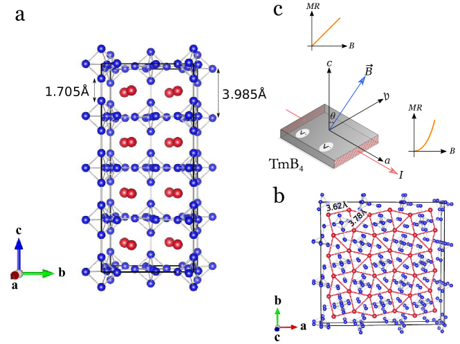
Figure 1: Structural and experimental considerations. (a) The alternating-layer crystal structure of TmB4. Four unit cells stacked along the c-axis are shown. The Tm (red) atom planes lie halfway between the B (blue) atom layers, which are separated by a distance of $3.985\text{\,}\mathrm{\SIUnitSymbolAngstrom}$. One type of boron lies exclusively within the boron plane, whereas the other type is part of the boron plane and an octahedral chain along the c-axis. (b) A unit cell of TmB4 viewed along the c-axis. The sub-lattice of Tm atoms maps to a topologically equivalent Shastry-Sutherland lattice structureShastry and Sutherland (1981) with perfect squares and nearly equilateral triangles of sides $3.62\text{\,}\mathrm{\SIUnitSymbolAngstrom}$ and $3.78\text{\,}\mathrm{\SIUnitSymbolAngstrom}$ respectively. The crystal structure of TmB4 is prepared using VESTAMomma and Izumi (2011). (c) A schematic of the experimental arrangement and main results. $\theta$ is the tilt angle between B and the crystal c-axis. The excitation current I is applied parallel to the ab-plane of the crystal, indicated in red, while the voltage drop is measured across the two voltage contacts, V$\,{}^{+}$ and V$\,{}^{-}$. The MR(B) is linear for $\theta=$0\text{\,}\mathrm{\SIUnitSymbolDegree}$$ and tunable to quadratic for $\theta=$90\text{\,}\mathrm{\SIUnitSymbolDegree}$$.

The low-temperature magnetic measurements carried out earlierSiemensmeyer et al. (2008); Gabáni et al. (2008); Wierschem et al. (2015); Sunku et al. (2016) on TmB4 revealed a rich phase diagram with multiple ground states for B applied along the c-axis. The ground state is antiferromagnetic (AFM), up to $T=$9.9\text{\,}\mathrm{K}$$ (for $B=$0\text{\,}\mathrm{T}$$) and $B=$1.4\text{\,}\mathrm{T}$$ (for $T\leq$8\text{\,}\mathrm{K}$$). At higher values of B and T, the system evolves to various other magnetic ground states, viz. a narrow fractional plateau phase (FPP), a wide half plateau phase, a modulated phase, and a high-field paramagnetic phaseSiemensmeyer et al. (2008); Gabáni et al. (2008); Wierschem et al. (2015); Sunku et al. (2016). Recently, specific heat measurements described FPP not as a distinct thermodynamic ground state of TmB4, but rather as being degenerate with the AFM phaseTrinh et al. (2018). Understanding of the various magnetic ground states in TmB4 has been at the forefront of extensive experimental and theoretical researchFisk et al. (1981); Yoshii et al. (2006); Siemensmeyer et al. (2008); Gabáni et al. (2008); Suzuki et al. (2010); Dublenych (2012); Wierschem et al. (2015); Sunku et al. (2016); Ye et al. (2017); Trinh et al. (2018), although transport propertiesGabáni et al. (2008); Sunku et al. (2016); Ye et al. (2017) are relatively less studied. Our previous magnetotransport investigationSunku et al. (2016) revealed huge, non-saturating and hysteretic in-plane MR (900% at $7\text{\,}\mathrm{T}$ for $2\text{\,}\mathrm{K}$) with signatures of unconventional anomalous Hall effect Sunku et al. (2016). The large MR along with negative Hall coefficient suggestSunku et al. (2016); Shekhar et al. (2015) that the carriers have high electronic $\mu\sim$$2.9\text{\,}\mathrm{m}^{2}\mathrm{V}^{-1}\mathrm{-}\mathrm{s}^{-1}$ at $2\text{\,}\mathrm{K}$.

II Experiment

Here, we focus on angle-dependent low-temperature magnetotransport experiments in TmB4 in its AFM phase ($B\leq$1.3\text{\,}\mathrm{T}$$ and $T\leq$5\text{\,}\mathrm{K}$$). A schematic of the experimental arrangement and the main result of this work are shown in fig. 1(c), where $\theta$ is the tilt angle between B and c-axis. We find an unexpected linear MR, tunable to quadratic by varying $\theta$. Single crystals of TmB4 were grown in a solution growth method using Al solution. Details of the crystal growth can be found elsewhereWierschem et al. (2015). For MR measurements, the crystal was orientedSunku et al. (2016) and cut into pieces with its faces along (001) direction using a tungsten wire. A rectangular piece of dimensions $\sim$0.434\text{\,}\mathrm{mm}$\times$0.516\text{\,}\mathrm{mm}$\times$0.226\text{\,}\mathrm{mm}$$ (weighing $\sim$0.35\text{\,}\mathrm{mg}$$) has been used for the measurements. The measurement was done in a standard four point probe method using a Quantum Design Physical Property Measurement System (PPMS). The contacts were made with electrically conductive silver epoxy paste (EpoTeK E4110) and gold wires of diameter $25\text{\,}\mathrm{\SIUnitSymbolMicro m}$ and $50\text{\,}\mathrm{\SIUnitSymbolMicro m}$ as connectors for voltage and current contacts respectively. All measurements were conducted well within the AFM phase ($B\leq$1.3\text{\,}\mathrm{T}$$ and $T\leq$5\text{\,}\mathrm{K}$$). The angle-dependent magnetotransport measurements were performed by placing the sample on a precision steeper controlled horizontal rotator puck, which can move around an axis perpendicular to B. The excitation current ($1.8\text{\,}\mathrm{mA}$ and $5.0\text{\,}\mathrm{mA}$) was applied parallel to the ab-plane and B was applied along various directions, relative to the crystal c-axis [see fig. 1(c)]. The linearity of current-voltage was ensured at both $300\text{\,}\mathrm{K}$ and $2\text{\,}\mathrm{K}$ prior to the magnetotransport measurements. We found in all cases that the MR is minimum at B = 0. The raw data of MR was then symmetrized to reflect the expected B to $-\textit{B}$ invariance, and is plotted in fig. 3(a). For the anisotropic magnetoresistance (AMR) measurements, R was measured as the sample was rotated continuously at a fixed B and T.

III Results and Discussions

Figure 2 depicts the metallicSunku et al. (2016) T dependence of the in-plane resistivity ($\rho_{ab}$) of TmB4 in a longitudinal ($B\parallel c$-axis) field with varying field strengths. At room temperatureSunku et al. (2016), the zero-field resistivity, $\rho_{ab}(B=0)$ is $5\text{\times}{10}^{-7}\text{\,}\mathrm{\SIUnitSymbolOhm}\text{\,}\mathrm{m}$ and decreases monotonically with decreasing T down to $12.9\text{\times}{10}^{-9}\text{\,}\mathrm{\SIUnitSymbolOhm}\text{\,}\mathrm{m}$ at $2\text{\,}\mathrm{K}$ giving residual resistivity ratio (RRR=$\frac{\rho_{300K}}{\rho_{2K}}$) = $38$. The RRR value is either comparable or even slightly higher than the previously studied TmB4 crystalsYe et al. (2017); Gabáni et al. (2008), suggesting a good quality crystal with a moderate amount of impurity. At $B=0$, the ratio of $\rho_{ab}$ to the c-axis resistivitySunku et al. (2016), $\rho_{c}$, is 0.454 at $2\text{\,}\mathrm{K}$. Loss of spin-disorder-scattering causes a sudden drop in $\rho_{ab}$ at $11.9\text{\,}\mathrm{K}$ (at $\textit{B}=0$) as the system undergoes an magnetic phase transition from the paramagnetic to the modulated phase. Following this second order phase transition, a first order phase transition appears at $9.9\text{\,}\mathrm{K}$ ($\textit{B}=0$) as the system moves from the magnetically ordered modulated phase to AFM state. Under B, these transition-Ts shift to lower values.

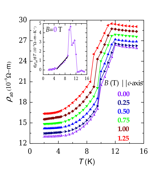
Figure 2: The temperature and field dependence of electrical resistivity ($\rho$) in the TmB4 single crystal. Plots of in-plane electrical resistivity ($\rho_{\textit{ab}}$), measured in various B, applied parallel to the crystal c-axis, against T. At $B=0$, the transition from the paramagnetic state to modulated state occurs at $11.9\text{\,}\mathrm{K}$ and transition from modulated phase to AFM phase occurs at $9.9\text{\,}\mathrm{K}$. $\rho_{\textit{ab}}$ increases and transition temperature decreases as B is increased. For the angle-dependent magnetotransport measurements, we consider the lower part ($2\leq\textit{T}\,($\mathrm{K}$)\leq 5$) of the $\rho_{\textit{ab}}$ – T curve. The lines are to guide the eye. Inset: T-derivative of $\rho_{\textit{ab}}(B=0)$ against T shows two maxima at the point of inflections of $\rho_{\textit{ab}}$ – T, implying the phase transitions. The abscissa of the inset has the same label as the main panel. The black solid line is the linear fit to the experimental data, signifying a T² dependence of $\rho_{\textit{ab}}$, in accordance with the Fermi liquid behavior.

As shown in the inset of fig. 2, zero-field $\frac{d\rho_{ab}}{dT}$ shows maxima at $T=$9.9\text{\,}\mathrm{K}$$ and $11.9\text{\,}\mathrm{K}$, indicative of the above-mentioned phase transitions. For $T\leq$9\text{\,}\mathrm{K}$$, $\frac{d\rho_{ab}}{dT}$ decreases linearly with decreasing T down to $4\text{\,}\mathrm{K}$, implying a $T^{2}$ variation of resistivity and is almost T independent in the lower T regime. This $T^{2}$ dependence of resistivity at low T, in a metal with magnetic ordering can arise either from $e-e$ scattering or scattering of conduction electrons from magnons Goodings (1963). A dominant $e-$magnon contribution results in a negative MR due to the suppression of magnonsMadduri and Kaul (2017) under B. However, unlike magnetic metals, TmB4 exhibits a positive MR and $\rho_{ab}$ increases with B (fig. 2). This rules out scattering from magnons as the primary source of resistivity in TmB4 and only $e-e$ scattering persists in accordance with Fermi liquid theory  ($\rho_{ab}=\rho_{0}+\beta T^{2}$, where $\rho_{0}$ is the residual resistivity). $\rho_{c}(T)$ also follows a similar $T^{2}$ behaviorSunku et al. (2016). The coefficient $\beta$ is inversely proportional to Fermi temperature and is set by the exponent of T rather than the residual resistivityLin et al. (2015). While for the in-plane transport, $\beta=$1.6\text{\times}{10}^{-10}\text{\,}\mathrm{\SIUnitSymbolOhm}\,\mathrm{m}\,\mathrm{K}^{-2}$$, its out-of-plane value is $83\text{\times}{10}^{-10}\text{\,}\mathrm{\SIUnitSymbolOhm}\,\mathrm{m}\,\mathrm{K}^{-2}$.

Figure 3(a) shows a set of normalized MR(B) isotherms of TmB4 with $\theta=$0\text{\,}\mathrm{\SIUnitSymbolDegree}$$ to $90\text{\,}\mathrm{\SIUnitSymbolDegree}$, measured at $T=$3\text{\,}\mathrm{K}$$. Here, $0\text{\,}\mathrm{\SIUnitSymbolDegree}$ ($90\text{\,}\mathrm{\SIUnitSymbolDegree}$) refers to a field B applied parallel (perpendicular) to the crystal’s c-axis (see fig. 1(c)). Unexpectedly, for $\theta=$0\text{\,}\mathrm{\SIUnitSymbolDegree}$$ to $45\text{\,}\mathrm{\SIUnitSymbolDegree}$ the MR response is linear all the way down to very small fields. The functional behavior of MR(B) changes gradually to quadratic as $\theta\to$90\text{\,}\mathrm{\SIUnitSymbolDegree}$$. Whilst the classical MR does not have any response when B is applied parallel to the excitation current, we observed a close to quadratic growth of MR for $B\parallel I\parallel ab$. The change in MR over the B-range ($\theta=$90\text{\,}\mathrm{\SIUnitSymbolDegree}$$) is less than 50% of that observed for $\theta=$0\text{\,}\mathrm{\SIUnitSymbolDegree}$$. MR ($\textit{B}=$1.3\text{\,}\mathrm{T}$$) is maximum for $\theta=$0\text{\,}\mathrm{\SIUnitSymbolDegree}$$ ($\approx$ 25%) and minimum ($\approx$ 10.3%) for $\theta=$90\text{\,}\mathrm{\SIUnitSymbolDegree}$$. MR(B) essentially shows similar features at other temperatures in the AFM phase. One of the notable features of the LMR in TmB4 is that it persists down to lowest applied field, without showing any signature of crossover to a quadratic behavior with change in B, as observed in CaMnBi2Wang et al. (2012a) InAsHu and Rosenbaum (2008), 2DEGAamir et al. (2012) and CrAsNiu et al. (2017). Instead, this LMR is similar to the super-linear MR behavior observed in non-stoichiometric silver chalcogenidesXu et al. (1997) , BiYang et al. (1999), WTe2Zhao et al. (2015) and rare-earth diantimonidesBud’ko et al. (1998). The slope of $\rho_{ab}(B,$0\text{\,}\mathrm{\SIUnitSymbolDegree}$)$ is $(2.21\pm 0.01)\text{\times}{10}^{-9}\text{\,}\mathrm{\SIUnitSymbolOhm}\,\mathrm{m}\,\mathrm{T}^{-1}$ and almost T-independent, suggesting the MR is not due to the phonon scattering Hu and Rosenbaum (2008).

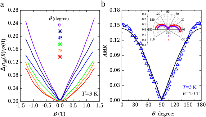
Figure 3: Angular dependence of MR. (a) A generic MR(B) isotherm measured at $\textit{T}=$3\text{\,}\mathrm{K}$$, under various magnetic field directions. $0\text{\,}\mathrm{\SIUnitSymbolDegree}$ ($90\text{\,}\mathrm{\SIUnitSymbolDegree}$) refers to whether B is applied parallel (perpendicular) to the crystal’s c-axis. A linear MR can be seen for $\theta=$0\text{\,}\mathrm{\SIUnitSymbolDegree}$$, which gradually moves to a quadratic form for $\theta=$90\text{\,}\mathrm{\SIUnitSymbolDegree}$$. The MR is anisotropic. For $\textit{B}=$1.3\text{\,}\mathrm{T}$$, the MR is $\approx$ 25% at $\theta=$0\text{\,}\mathrm{\SIUnitSymbolDegree}$$, whereas it is $\approx$ 10.3% for $\theta=$90\text{\,}\mathrm{\SIUnitSymbolDegree}$$. (b) The $\theta$ variation of anisotropic magnetoresistance (AMR) (see text) measured at $\textit{B}=$1.0\text{\,}\mathrm{T}$$ and $\textit{T}=$3\text{\,}\mathrm{K}$$. The experimental data can be described by a $\absolutevalue{\cos\theta}$ function (solid line) indicating a quasi-2D FSWang et al. (2012a); Zhao et al. (2015). Inset: Polar plot of AMR($\theta$) measured at $\textit{T}=$2\text{\,}\mathrm{K}$$ and $5\text{\,}\mathrm{K}$, at $\textit{B}=$1.3\text{\,}\mathrm{T}$$. The AMR shows two-lobes over the full range of $\theta$, suggesting a two-fold symmetry.

Furthermore, we find MR to be anisotropic. We define anisotropic magnetoresistance (AMR$(\theta)$) as $\frac{R(\theta)-R_{\mathrm{min}}}{R_{\mathrm{min}}}$, where $R(\theta)$ is the resistance at any $\theta$, measured at a constant $B$ and $T$, and $R_{\mathrm{min}}$ is the minimum resistance obtained as $\theta$ is varied. In fig. 3(b), we show the variation of AMR$(\theta)$ at $T=$3\text{\,}\mathrm{K}$$ for $B=$1.0\text{\,}\mathrm{T}$$. AMR is maximum for $B\parallel c$-axis and diminishes as B is rotated away from the $c$-axis. The data can be satisfactorily fit with a $\absolutevalue{\cos\theta}$ dependence. This suggests a (quasi-)$2D$ FSPippard (1989); Wang et al. (2012a); Zhao et al. (2015), where MR responds to the perpendicular component of the applied field, $B~{}\absolutevalue{\cos\theta}$. The anisotropic MR further suggests an anisotropy in the electronic effective massZhao et al. (2015). AMR shows two-fold symmetry (inset fig. 3(b)).

To quantify the evolution of MR from linear to quadratic, we fit MR$(B,\theta)$ to $\bigl{(}\frac{B}{B_{0}}\bigr{)}^{p}$. A representative $MR(B)$ plot (in double logarithmic scale), measured at $4\text{\,}\mathrm{K}$ for different $\theta$ values, is shown in fig. 4(a). For $\theta=$0\text{\,}\mathrm{\SIUnitSymbolDegree}$$, $\textit{p}\cong 1$ and gradually grows to $p\approx 2$ (varies between 1.5 to 1.9, for different Ts) for $\theta=$90\text{\,}\mathrm{\SIUnitSymbolDegree}$$ (fig. 4(b)). Crucially, $p(\theta)$ varies similarly at all temperatures and has a negligible T-dependence within the AFM phase (fig. 4(b)).

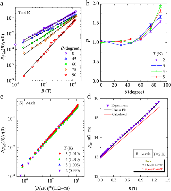
Figure 4: Analysis of the magnetoresistance data for TmB4. (a) Magnetoresistance isotherm, measured at $\textit{T}=$4\text{\,}\mathrm{K}$$, under five different field orientations, shown in a double logarithmic representation. The linearity in the log-log plot suggests a power law behavior, $\textit{MR}=\bigl{(}\frac{B}{B_{0}}\bigr{)}^{p}$. The solid lines are the fit of the experimental data to the power law. (b) The variation of the exponent, p, with $\theta$, for various Ts. For $\theta=$0\text{\,}\mathrm{\SIUnitSymbolDegree}$$, p is close to 1, suggesting linear MR and gradually moves to a value close to 2, for $\theta=$90\text{\,}\mathrm{\SIUnitSymbolDegree}$$. The error for determining the value of $p$ from the fit (a) is $\sim$ 0.01 and shown in the plot. $p$ varies in a similar manner for all Ts. The lines are to guide the eye. (c) T-scaling (Kohler rule) of MR for B along c-axis. The values of $m$ used to scale the different T MR data are mentioned in the parenthesis. (d) Comparison of the experimental data (violet) and theoretical (red) plot. The experimental data was obtained for $B\parallel c$-axis configuration and measured at $T=$2\text{\,}\mathrm{K}$$. The black solid line is the linear fit to the experimental data. The theoretical curve was calculated from Eq. 1 using the values of $N_{i}$ and $n_{e}$ (see text). The values of both slopes (inset) agree within 7%.

MR (B, $\theta=0$) data at different Ts can be scaled using the Kohler relation, $\textit{MR}=\alpha(\textit{T})\bigl{[}\frac{B}{\rho(0)}\bigr{]}^{m}$ (fig. 4(c)). The scaling suggests that the carriers with single salient relaxation timePippard (1989) govern magnetotransport for $\textit{B}\parallel\textit{c}$-axis in the AFM phase. Furthermore, this robust T-scaling, using a single $\alpha$, adds credence to the relative T-insensitivity of LMR and implies negligible phononic contributions. Therefore, the measured MR is primarily governed by scattering of conduction electrons by impurities.

The origin of LMR in TmB4 is not entirely clear, but it is plausible that Abrikosov’s theory of quantum linear MRAbrikosov (1969, 1998, 1999, 2000) can be invoked for this purpose, considering the topology of the Fermi surface(FS) of TmB4 Shin et al. (2017). The presence of two symmetry related small pockets (as evident from the spin-polarized DFT calculation using GGA+U method) in the $k_{x}-k_{y}$ plane of the Brillouin Zone (BZ) along the $\Gamma-X$ direction (labeled $\Gamma^{\prime}$ in fig. 5), with an approximately linear crossing of two bands at the Fermi energy, $E_{F}$ (within the numerical accuracy) (Fig. 5) is of particular interest here. The low density and small effective mass of the carriers due to the linear band crossing, ensure that they can be confined to the lowest Landau level, and thus reach the extreme quantum limit even at small (longitudinal) applied fields. This results to a LMR Abrikosov (1969, 1998, 1999, 2000) and is given by,

$$\rho_{xx}=\frac{N_{i}B}{\pi cen_{e}^{2}}$$ (1)

provided that the carrier concentration ($n_{e}$) satisfies $n_{e}\lesssim\left(\frac{m_{zz}}{m_{xy}}\right)^{\frac{1}{2}}\left(\frac{eB}{\hbar c}\right)^{\frac{3}{2}}$, $m_{zz}$ and $m_{xy}$ are the effective mass of the carriers for motion along $k_{z}$ and in the $k_{x}-k_{y}$ plane, respectively and $N_{i}$ ($\ll n_{e}$) is the density of static scattering centers.

The low effective mass of the carriers further gives a T-limit for lowest Landau level confinement (see Supplementary information) which is indeed satisfied in our experiments. At small fields, due to the low effective mass of the electrons from the Fermi pockets, and consequently their high cyclotron frequency, the linear contribution dominates over the usual quadratic MR from the rest of the FSAbrikosov (2000). Using the values of carrier density and their effective masses estimated from band structure calculations, as well as impurity concentrations from sample preparation conditions, Eq. 1 yields an MR(B) that is in agreement with the experimentally observed magnetotransport data in TmB4 (fig. 4(d)). The compliance of MR (B, $\theta=0$) to Kohler scaling provides further support to the assumption that magnetotransport at small longitudinal fields is dominated by charge carriers from identical Fermi pockets.

The mechanism identified above explains another intriguing feature of TmB4 – the absence of Shubnikov-de Haas (SdH) oscillations in the observed MR data. Since the extreme quantum limit is already reached at very small fields for the pocket under consideration, there are no Landau level crossings of the FS with increasing field, and consequently no SdH oscillations. In principle, the SdH oscillations should be observed for B along ab-plane, but we could not reach the required B, due to strong magnetic fluctuations and experimental limitations.

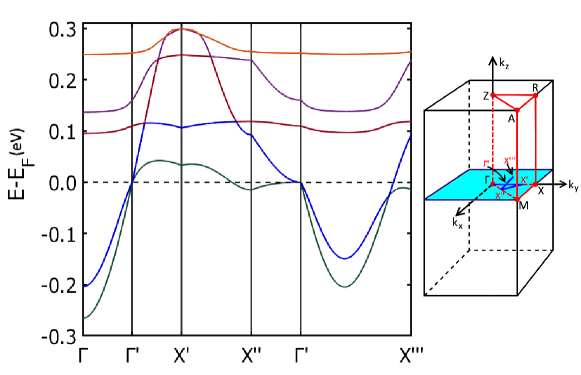
Figure 5: Band structure for TmB4 from the spin polarized DFT calculation using GGA+U method, shows dispersion in the ab plane. The right panel shows the path (in blue) taken in the BZ, $\Gamma$–$\Gamma^{\prime}$–X^′–X^′′–$\Gamma^{\prime}$–X^′′′. A band crossing is observed exactly at $E_{F}$ with linear dispersion in the $k_{x}-k_{y}$ plane at $\Gamma^{\prime}$.

Finally, the absence of LMR for transverse magnetic fields can also be understood from the anisotropic FS topology. Being a layered material, the small pockets in the $k_{x}-k_{y}$ plane of TmB4 are believed to originate from the overlap of bands close to the FS due to the inter-layer coupling. Consequently, there are no such pockets at corresponding points on the surface of the BZ in the XY plane. Since magnetotransport of a solid is governed by the external cross section of the FS along the field directionWang et al. (2012a), only the quadratic contribution of the total conductivity persists for B applied along the principal plane. This picture, based on the topology of the FS of TmB4, qualitatively explains the experimental observation of tuning MR from quadratic to linear as the field direction is rotated.

It should be noted that the above discussion is a plausible, rather than a rigorous elucidation for the origin of LMR in TmB4. The present explanation depends crucially on the existence of a linear band crossing very close to the FS in the $k_{x}-k_{y}$ plane. Unfortunately, DFT is unable to capture the effects of strong correlations with high accuracy, therefore one must regard the interpretation as tentative and a much rigorous analytic calculation is indeed required for better insight into the problem. However, it is interesting that the present approach based on anisotropic FS topology within the quantum linear magnetoresistance framework is consistent with the experimental observations. It thus provides a useful platform for further studies of this compelling phenomenon.

IV Summary

In summary, we have discussed the tuning of MR from linear to quadratic in single crystalline metal, TmB4, by rotating B relative to the crystal c-axis. We give a plausible explanation of the LMR in this metallic system based on its FS topology within the quantum linear magnetoresistance picture, which predominantly holds true for semimetals and topological insulators. We argued that the linear dispersion near $E_{F}$ and the subsequent Fermi pocket in the FS of TmB4, arising from its layered structure, give rise to a LMR in an otherwise normal metal and its complex FS topology governs the tuning of in-plane MR from quadratic to linear.

References

- Niu et al. (2017) Q. Niu, W. C. Yu, K. Y. Yip, Z. L. Lim, H. Kotegawa, E. Matsuoka, H. Sugawara, H. Tou, Y. Yanase, and S. K. Goh, Nat. Commun. 8, 15358 (2017).
- Pippard (1989) A. B. Pippard, Magnetoresistance in Metals (Cambridge University Press, Cambridge, USA, 1989) p. 253.
- Parish and Littlewood (2003) M. M. Parish and P. B. Littlewood, Nature 426, 162 (2003).
- Parish and Littlewood (2005) M. M. Parish and P. B. Littlewood, Phys. Rev. B 72, 094417 (2005).
- Yan et al. (2013) Y. Yan, L.-X. Wang, D.-P. Yu, and Z.-M. Liao, Appl. Phys. Lett. 103, 033106 (2013).
- Alekseev et al. (2015) P. S. Alekseev, A. P. Dmitriev, I. V. Gornyi, V. Y. Kachorovskii, B. N. Narozhny, M. Schütt, and M. Titov, Phys. Rev. Lett. 114, 156601 (2015).
- Narayanan et al. (2015) A. Narayanan, M. D. Watson, S. F. Blake, N. Bruyant, L. Drigo, Y. L. Chen, D. Prabhakaran, B. Yan, C. Felser, T. Kong, P. C. Canfield, and A. I. Coldea, Phys. Rev. Lett. 114, 117201 (2015).
- Song et al. (2015) J. C. W. Song, G. Refael, and P. A. Lee, Phys. Rev. B 92, 180204 (2015).
- Kisslinger et al. (2017) F. Kisslinger, C. Ott, and H. B. Weber, Phys. Rev. B 95, 024204 (2017).
- Khouri et al. (2016) T. Khouri, U. Zeitler, C. Reichl, W. Wegscheider, N. E. Hussey, S. Wiedmann, and J. C. Maan, Phys. Rev. Lett. 117, 256601 (2016).
- Abrikosov (1969) A. A. Abrikosov, Sov. Phys. JETP 29, 746 (1969).
- Abrikosov (1998) A. A. Abrikosov, Phys. Rev. B 58, 2788 (1998).
- Liang et al. (2015) T. Liang, Q. Gibson, M. N. Ali, M. Liu, R. J. Cava, and N. P. Ong, Nat. Mater. 14, 280 (2015).
- Yang et al. (1999) F. Y. Yang, K. Liu, K. Hong, D. H. Reich, P. C. Searson, and C. L. Chien, Science 284, 1335 (1999).
- Xu et al. (1997) R. Xu, A. Husmann, T. F. Rosenbaum, M.-L. Saboungi, J. E. Enderby, and P. B. Littlewood, Nature 390, 57 (1997).
- Kopelevich et al. (2013) Y. Kopelevich, R. R. da Silva, B. C. Camargo, and A. S. Alexandrov, J. Phys. Condens. Matter 25, 466004 (2013).
- Friedman et al. (2010) A. L. Friedman, J. L. Tedesco, P. M. Campbell, J. C. Culbertson, E. Aifer, F. K. Perkins, R. L. Myers-Ward, J. K. Hite, C. R. Eddy, G. G. Jernigan, and D. K. Gaskill, Nano Lett. 10, 3962 (2010).
- Wang et al. (2012a) K. Wang, D. Graf, L. Wang, H. Lei, S. W. Tozer, and C. Petrovic, Phys. Rev. B 85, 041101 (2012a).
- Delmo et al. (2009) M. P. Delmo, S. Yamamoto, S. Kasai, T. Ono, and K. Kobayashi, Nature 457, 1112 (2009).
- Hu and Rosenbaum (2008) J. Hu and T. F. Rosenbaum, Nat. Mater. 7, 697 (2008).
- Wang et al. (2012b) X. Wang, Y. Du, S. Dou, and C. Zhang, Phys. Rev. Lett. 108, 266806 (2012b).
- Barua et al. (2014) S. Barua, K. P. Rajeev, and A. K. Gupta, J. Phys. Condens. Matter 27, 015601 (2014).
- Hayes et al. (2016) I. M. Hayes, R. D. McDonald, N. P. Breznay, T. Helm, P. J. W. Moll, A. S. Mark Wartenbe, and J. G. Analytis, Nat. Phys. 12, 916 (2016).
- Abrikosov (1999) A. A. Abrikosov, Phys. Rev. B 60, 4231 (1999).
- Zhao et al. (2015) Y. Zhao, H. Liu, J. Yan, W. An, J. Liu, X. Zhang, H. Wang, Y. Liu, H. Jiang, Q. Li, Y. Wang, X.-Z. Li, D. Mandrus, X. C. Xie, M. Pan, and J. Wang, Phys. Rev. B 92, 041104 (2015).
- Aamir et al. (2012) M. A. Aamir, S. Goswami, M. Baenninger, V. Tripathi, M. Pepper, I. Farrer, D. A. Ritchie, and A. Ghosh, Phys. Rev. B 86, 081203 (2012).
- Bud’ko et al. (1998) S. L. Bud’ko, P. C. Canfield, C. H. Mielke, and A. H. Lacerda, Phys. Rev. B 57, 13624 (1998).
- Myers et al. (1999) K. D. Myers, S. L. Bud’ko, I. R. Fisher, Z. Islam, H. Kleinke, A. H. Lacerda, and P. C. Canfield, J. Magn. Magn. Mater 205, 27 (1999).
- Shastry and Sutherland (1981) B. S. Shastry and B. Sutherland, Physica B+C 108, 1069 (1981).
- Michimura et al. (2009) S. Michimura, A. Shigekawa, F. Iga, T. Takabatake, and K. Ohoyama, Jour. of the Phys. Soc. of Jpn. 78, 024707 (2009).
- Shin et al. (2017) J. Shin, Z. Schlesinger, and B. S. Shastry, Phys. Rev. B 95, 205140 (2017).
- Momma and Izumi (2011) K. Momma and F. Izumi, J. Appl. Cryst. 44, 1272 (2011).
- Siemensmeyer et al. (2008) K. Siemensmeyer, E. Wulf, H.-J. Mikeska, K. Flachbart, S. Gabáni, S. Mat’aš, P. Priputen, A. Efdokimova, and N. Shitsevalova, Phys. Rev. Lett. 101, 177201 (2008).
- Gabáni et al. (2008) S. Gabáni, S. Mat’aš, P. Priputen, K. Flachbart, K. Siemensmeyer, E. Wulf, A. Evdokimova, and N. Shitsevalova, Acta. Phys. Pol. A 113, 227 (2008).
- Wierschem et al. (2015) K. Wierschem, S. S. Sunku, T. Kong, T. Ito, P. C. Canfield, C. Panagopoulos, and P. Sengupta, Phys. Rev. B 92, 214433 (2015).
- Sunku et al. (2016) S. S. Sunku, T. Kong, T. Ito, P. C. Canfield, B. S. Shastry, P. Sengupta, and C. Panagopoulos, Phys. Rev. B 93, 174408 (2016).
- Trinh et al. (2018) J. Trinh, S. Mitra, C. Panagopoulos, T. Kong, P. C. Canfield, and A. P. Ramirez, Phys. Rev. Lett. 121, 167203 (2018).
- Fisk et al. (1981) Z. Fisk, M. B. Maple, D. C. Johnston, and L. D. Woolf, Solid State Commun. 39, 1189 (1981).
- Yoshii et al. (2006) S. Yoshii, T. Yamamoto, M. Hagiwara, A. Shigekawa, S. Michimura, F. Iga, T. Takabatake, and K. Kindo, J. Phys. Conf. Ser. 51, 59 (2006).
- Suzuki et al. (2010) T. Suzuki, Y. Tomita, N. Kawashima, and P. Sengupta, Phys. Rev. B 82, 214404 (2010).
- Dublenych (2012) Y. I. Dublenych, Phys. Rev. Lett. 109, 167202 (2012).
- Ye et al. (2017) L. Ye, T. Suzuki, and J. G. Checkelsky, Phys. Rev. B 95, 174405 (2017).
- Shekhar et al. (2015) C. Shekhar, A. K. Nayak, Y. Sun, M. Schmidt, M. Nicklas, I. Leermakers, U. Zeitler, Y. Skourski, J. Wosnitza, Z. Liu, Y. Chen, W. Schnelle, H. Borrmann, Y. Grin, C. Felser, and B. Yan, Nat. Phys. 11, 645 (2015).
- Goodings (1963) D. A. Goodings, Phys. Rev. 132, 542 (1963).
- Madduri and Kaul (2017) P. V. P. Madduri and S. N. Kaul, Phys. Rev. B 95, 184402 (2017).
- Lin et al. (2015) X. Lin, B. Fauqué, and K. Behnia, Science 349, 945 (2015).
- Abrikosov (2000) A. A. Abrikosov, Europhys. Lett. 49, 789 (2000).
- Note (1) For calculation details please see Ref. 31.
- Note (2) Above this T-value, we previously observed a quadratic MR for -axis. Please see Ref.36 for details.
- Note (3) Estimating is tricky, since the pocket is reduced to a point in the zero-field first principle calculations. However, as a rough estimate, we can use the calculated value for the other smallest Fermi pocketsShin et al. (2017), viz., .).
- Note (4) A comparison between the residual resistivity (RR) of our sample and similarly grown \ceTmB4 crystals with known impurity densityOkada et al. (1994) allows us to estimate (assuming the RR arises solely from scattering of electrons off impurity), as . For details, see Supplementary information.
- Okada et al. (1994) S. Okada, K. Kudou, Y. Yu, and T. Lundström, Jpn. J. Appl. Phys 33, 2663 (1994).